Sage Journals: Discover world-class research

Abstract

This article discusses the highly autonomous robotic search and localization of radiation sources in outdoor environments. The cooperation between a human operator, an unmanned aerial vehicle, and an unmanned ground vehicle is used to render the given mission highly effective, in accordance with the idea that the search for potential radiation sources should be fast, precise, and reliable. Each of the components assumes its own role in the mission; the unmanned aerial vehicle (in our case, a multirotor) is responsible for fast data acquisition to create an accurate orthophoto and terrain map of the zone of interest. Aerial imagery is georeferenced directly, using an onboard sensor system, and no ground markers are required. The unmanned aerial vehicle can also perform rough radiation measurement, if necessary. Since the map contains three-dimensional information about the environment, algorithms to compute the spatial gradient, which represents the rideability, can be designed. Based on the primary aerial map, the human operator defines the area of interest to be examined by the applied unmanned ground vehicle carrying highly sensitive gamma-radiation probe/probes. As the actual survey typically embodies the most time-consuming problem within the mission, major emphasis is put on optimizing the unmanned ground vehicle trajectory planning; however, the dual-probe (differential) approach to facilitate directional sensitivity also finds use in the given context. The unmanned ground vehicle path planning from the pre-mission position to the center of the area of interest is carried out in the automated mode, similarly to the previously mentioned steps. Although the human operator remains indispensable, most of the tasks are performed autonomously, thus substantially reducing the load on the operator to enable them to focus on other actions during the search mission. Although gamma radiation is used as the demonstrator, most of the proposed algorithms and tasks are applicable on a markedly wider basis, including, for example, chemical, biological, radiological, and nuclear missions and environmental measurement tasks.

Keywords

Mobile robot unmanned aerial vehicle unmanned ground vehicle gamma radiation localization aerial mapping self-localization navigation robot cooperation

Introduction

At present, new security challenges appear within multiple related fields and disciplines. In this connection, the advancement in modern warfare suggests that chemical, biological, radiological, and nuclear defense will assume increasing importance. The US Department of Health and Human Services defines several types of terrorist attacks involving sources of ionizing radiation¹; the perpetrators of such acts may rely on dirty bombs, devices having the potential to disperse radioactive material in urban zones. As radiological sources are commonly present in medical or scientific facilities, they appear rather vulnerable in terms of becoming a target or an instrument of criminal practices.² In any case of such misuse, it would be vital to localize and dispose the dangerous sources without unnecessary delay.

Current scientific literature outlines various methods to perform the actual retrieval and elimination operations; for instance, one of the conventional techniques relies on airborne spectrometry, where the detectors are carried by a helicopter through the region of interest (ROI) along a regular trajectory. An example of this approach was found Johsi et al.³ The advantage of such a procedure consists in the possibility of quickly exploring a relatively large region, while the main drawback is the low accuracy of estimating the hotspot locations. However, a detector can also be attached to an unmanned aerial vehicle (UAV), as presented in research reports by Hartman et al.⁴ and Aleotti et al.⁵ The benefits and disadvantages are similar to those characterizing the use of a helicopter; in this connection, UAVs nevertheless exhibit smaller payloads and shorter flying ranges, although they also feature lower initial costs.

If a high localization accuracy is required, ground-based assets have to be employed. The actual localization should not be performed by humans due to health risks, and as an unmanned ground vehicle (UGV) is less prone to radiation damage, it finds application in such reconnaissance tasks. Using UGVs in the discussed domain is demonstrated in articles.^6

–10 A custom solution offering a high accuracy of the localization of gamma radiation hotspots is introduced within the present paper.

The proposed solution consists of an aerial and a ground platform, both working in the semiautonomous mode. A UAV is utilized to acquire a three-dimensional (3-D) map of the ROI via photogrammetric techniques. The map assists a UGV to plan a trajectory along which the hotspots are searched. In addition, the UAV may carry a detector to provide general information related to the positions of the radiation hotspots. A central advantage of our approach lies in the fact that no prior environmental map is needed, and the goal rests in identifying a solution that overcomes the state-of-the-art methods in certain particular aspects.

The article is organized as follows. The “Methods” section discusses the methods and equipment employed, together with several localization algorithms; “Results” section offers an overview of the results achieved, including the performance, time efficiency, and accuracy typical of the individual maps and methods; and “Discussion” section compares the results with those outlined in the referenced literature, introducing the relevant advantages and disadvantages.

Methods

The following section presents the working scheme of the proposed system; both the UAV and the UGV are described in detail. The final part of this section introduces the algorithms used.

Process description

The sequence of steps to ensure information related to the gamma radiation hotspots is illustrated in Figure 1. The entire process is controlled by a human operator (user).

Figure 1.

The sequence of the operations forming the entire process.

At the initial stage, the operator has to plan a flight trajectory for the UAV to cover the potentially affected area; then, the UAV acquires images along the defined trajectory, and these are used to reconstruct the 3-D model of the area. The model assists the operator in selecting the proper ROI rideable for the UGV, considering the presence of possible radiation hotspots. The ROI is a polygon defined by a sequence of vertices.

The UGV is deployed near the border of the mapped area. First, the trajectory from the deployment position to the edge of the ROI is calculated to avoid the obstacles and slopes found by the UAV; subsequently, the operator chooses the UGV working mode. In general terms, two modes are available: mapping and localization. While the former procedure yields a map of the radiation distribution in the area, the latter one enables us to localize the radiation sources as quickly as possible; the corresponding data are then acquired in a suitable manner. Finally, the measurement is interpolated in order to provide either a map or a set of the sources’ coordinates, and the results are communicated to the operator.

Unmanned aerial vehicle

In aerial mapping, the benefit of UAVs consists in their fast and safe operation at a very reasonable price, especially when compared to manned aircraft. For this reason, UAVs are convenient primarily for the mapping of local areas as their operational time is rather limited; conversely, however, the vehicles can produce a refreshed map on a daily basis, thus significantly reducing the product cycle known from traditional mapping. UAVs have already proven useful in fields and disciplines, such as agriculture, civil engineering, archaelogy, or environmental and radiation mapping. Currently, projects are being executed which focus on direct radiation mapping via onboard sensors^4,11 and combine radiation mapping with UAV photogrammetry to facilitate 3-D surface reconstruction¹²; this article nevertheless aims to explore the potential for cooperation between UAVs and UGVs.

To perform the aerial mapping, we used a six-rotor DJI S800 Spreading Wings UAV fitted with a DJI (Shenzhen, China) Wookong M flight controller supporting an autonomous flight according to a given trajectory. As regards the experimental aicraft, the most important utility parameter was the payload limit of about 3 kg, which allowed us to carry the required equipment (see Table 1 for more parameters). The UAV comprises a custom-built multi-sensor system facilitating the direct georeferencing (DG) of aerial imagery (Figure 2), an operation that enables us to create a georeferenced orthophoto, point cloud, or digital elevation model (DEM) without requiring ground control points (GCPs).

Table 1.

The parameters of the UAV DJI S800 and the UGV Orpheus-X3.^16,30

Parameter	UAV	UGV
Dimensions	1.0 × 1.2 × 0.5 m³	1.0 × 0.6 × 0.4 m³
Weight	8 kg	51 kg
Operational time	10 min	120 min
Drive type	multi-rotor	wheel-differential
Operating speed	5 m/s	0.6 m/s
Maximum speed	26 m/s	4.2 m/s

UAV: unmanned aerial vehicle; UGV: unmanned ground vehicle.

Figure 2.

The DJI S800 UAV equipped with the multi-sensor system for DG. UAV: unmanned aerial vehicle; DG: direct georeferencing.

The multi-sensor system comprises a digital camera (Sony Alpha A7 [Sony Corporation, Tokyo, Japan]), a global navigation satellite system (GNSS) receiver (Trimble BD982 [Trimble Inc., Sunnyvale, CA, USA]), an inertial navigation system (INS; SBG Ellipse-E [SBG Systems S.A.S., Carriéres-sur-Seine, France]), and a single board computer (Banana Pi R1 [SinoVoip Co., Ltd, Shenzhen, China]; Figure 3). The GNSS receiver measures the position with centimeter-level accuracy when real-time kinematic (RTK) correction data are transmitted, and as it is equipped with two antennas for vector measurement, the device also measures the orientation around two axes. The position and orientation data are used as an auxiliary input for the INS, which provides data output at a frequency of up to 200 Hz. Since all the sensors are precisely synchronized, once an image has been captured, the position and orientation data are saved into the onboard solid-state drive (SSD) data storage (more parameters are contained in Table 2). The multi-sensor system mounted on the UAV is shown in Figure 2 and described in more detail in the study by Gabrlik et al.¹³

Figure 3.

The multi-sensor system for the UAV and ground station. UAV: unmanned aerial vehicle.

Table 2.

The parameters of the custom-built multi-sensor system for UAVs to enable the DG of aerial imagery.

Parameter	Value
Position accuracy (BD982)^*	horizontal: 8 mm; vertical: 15 mm
Attitude accuracy (Ellipse-E)^†	roll/pitch: 0.1°; heading: 0.4°
Camera resolution	6000 × 4000 pixel
Camera lens	15 mm
Operational time	120 min
Distance from base	1000 m
Dimensions	1.5 × 0.2 × 0.2 m³
Weight	2.6 kg

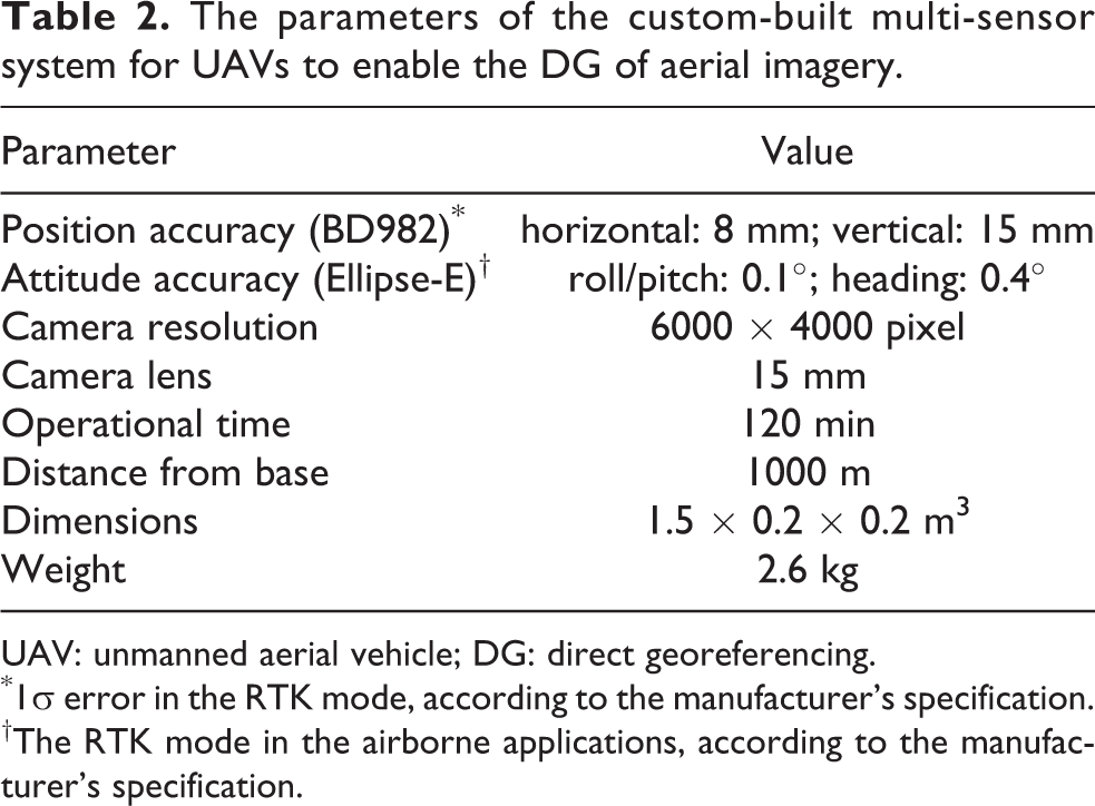
UAV: unmanned aerial vehicle; DG: direct georeferencing.

^*1σ error in the RTK mode, according to the manufacturer’s specification. ^†The RTK mode in the airborne applications, according to the manufacturer’s specification.

Both the position and the image data from the onboard sensors are processed using photogrammetric software (SW) Agisoft Photoscan Professional (version 1.3.1 build 4030). This SW integrates computer vision-based algorithms performing structure from motion to allow the surface reconstruction, and it offers two georeferencing options: indirect georeferencing (IG), using GCPs, and DG, utilizing onboard data. We may benefit from DG as the only approach to produce accurately georeferenced maps of areas inaccessible for humans (which is the case with radiation mapping). To achieve centimeter-level object accuracy, a method for calibrating the designed system was developed.¹⁴ The calibration process involves the field estimation of the lever arms and the synchronization delay between the camera shutter and the INS unit; these steps significantly increase the accuracy of the position measurement of the camera’s perspective center.

In our experiment, the UAV is used only for the aerial photogrammetry, enabling us to create a highly detailed, up-to-date orthophoto and DEM. These products are applicable for both the localization of the ROI and the UGV navigation. If the UAVs were equipped also with radiation detectors, it would locate the ROI more reliably.

Unmanned ground vehicle

The UGV is an Orpheus-X3 (LTR s.r.o., Brno, Czech Republic) civil reconnaissance robot, a four-wheeled midsize vehicle equipped with a sensor head carrying cameras. The robot has the ability to carry all the equipment needed for this type of mission, namely, devices to facilitate self-localization, gamma detectors with counting electronics, and a control module with the designed algorithms. The whole system, namely, the robot carrying the equipment, is represented in Figure 4. The basic parameters of the robot are shown in Table 1. The interconnection between the main components of Orpheus-X3 is shown in Figure 5. The robot is capable of autonomous driving. A simplified block scheme of all major modules for the robot motion control is drawn in Figure 6; all the blocks of this scheme will be described in detail within the following paragraphs.

Figure 4.

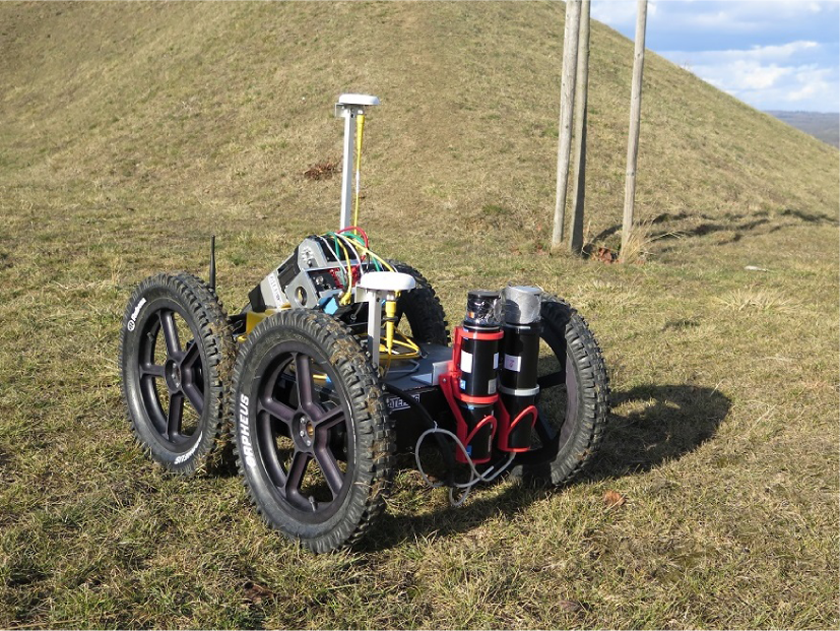
The Orpheus-X3 carrying the equipment.

Figure 5.

The interconnection of the components.

Figure 6.

The control diagram of the simplified robot drive.

In applications that require the autonomous motion control of a mobile robot, the self-localization task must be solved in real time. The self-localization module of the Orpheus-X3 mobile robot is designed exploiting the modular concept with real-time data output; such an approach allows the quick and easy integration of localization data from different sources. The data fusion is based on uncertainties of the input data. In standard missions, the self-localization module includes solutions from an RTK GNSS (Trimble BD982), a microelectromechanical system–based INS (SBG Ellipse-E), and wheel odometry (data from the motor drivers). One of the central advantages of an RTK GNSS is the high accuracy without any drift caused by the length of the measuring period or traveled distance. The applied RTK GNSS receiver can be connected to two antennas, allowing drift-less heading measurement from the position vector between the two antennas. The localization data from special methods (including, e.g. simultaneous localization and mapping) can also be integrated if the uncertainties of the values are known. In environments with a good open sky view, an RTK GNSS is usable as the only solution. To increase the robustness of the entire self-localization module, we may also employ some relative methods to bypass the time when the RTK solution is unavailable due to reasons such as reinitialization. The position estimation accuracy reaches the level of centimeters, and the orientation (azimuth) is better than 0.5° if the RTK solutions are fixed. As regards accuracy, more results are obtainable from the PhD thesis by Jilek.¹⁵

The Orpheus-X3 also integrates a navigation module (Figure 7) to control the robot motion, utilizing an externally computed requested trajectory. The trajectory is defined as a sequence of waypoints in the World Geodetic System 84 (WGS-84). The internal computational scheme of the navigation solution (block no. 1 in Figure 7) is presented in Figure 8. The robot motion parameters, such as the turning radius and maximum speeds, can be dynamically adjusted during a mission via an integrated application interface from the related hi-level control module. The sequence of waypoints is also dynamically modifiable from the path planner module during a mission. More information about the navigation algorithms is outlined in the study and PhD thesis by Jilek.^15,16

Figure 7.

The block scheme of the module.

Figure 8.

The scheme of the navigation solution solver.

The gamma radiation detection system comprises scintillation detectors and measuring electronics. A pair of 2-in. sodium iodide doped with thallium detectors are used as scintillators. The detectors are integrated with photomultiplier tubes having a standard 14-pin base. Multichannel analyzers NuNA MCB3 manufactured by NUVIA (Nuvia a.s., Trebic, Czech Republic) are used as the electronics; the analyzers ensure a high voltage source, a preamplifier, and analog-to-digital converter sampling and processing. The detector tubes are equipped with lead shielding, and one half of each spherical detector is covered with a 2-mm layer of lead facing the other detector. The reason for such a configuration is to intensify the directional sensitivity of the resulting detection system. The directional characteristics of the detectors placed on the robot are introduced in Figure 9; however, these remain valid only if the distance between the detector centers equals 106 mm.

Figure 9.

The directional characteristics of the detection system.

Optimal path to the area of interest

The terrain negotiability of a UGV is markedly affected by its actual slope pattern. In this context, it appears very helpful if the entire system can assist the operator in finding the shortest possible path to the target area from places accessible using the regular transport infrastructure. The main obstacles for a UGV are areas where the slope of the terrain exceeds the limit value of the given UGV. The slope map is computed from a DEM, which constitutes a product of UAV photogrammetry. The paths from the starting positions to the requested target are obtained using an A* algorithm¹⁷ in a binarized and down-sampled slope map; the down-sampling of the map is needed due to a significant reduction in the computational demands. The size of a cell in a down-sampled obstacle map should be slightly higher than the width of the applied UGV. Lowering this size below this limit has no effect because of the impossibility to pass through a corridor with the width of 1 pixel, whereas increasing it worsens the resolution and may cause the loss of the trajectory. The down-sampling algorithm must preserve the thin lines that represent high slopes in the terrain.

Another approach to reduce the computational demands consists in using lossless compression algorithms (e.g. quadtree¹⁸) on a primary hi-resolution binary map. These algorithms can also be employed in lossy compression applications, where the cell size of a leaf (the last level of the tree) is larger than in the original map. In the given case, however, the workflow must be changed, with the primary binary map packed using a quadtree algorithm at the start of the data processing. Furthermore, the path planning algorithm must be modified to natively handle the compressed data without fully expanding to an equidistant grid. Compared to the basic down-sampling, this procedure significantly reduces the number of points needed to travel through a path planning algorithm while keeping the same resolution of the map. Such an optimization then markedly affects the computational demands. Due to the negligible duration (only several seconds) of the trajectory planning operation as opposed to the DEM calculation time (which amounts to several hours if a computing grid is not utilized), the benefits of more advanced obstacle map compression techniques are unimportant in the described application.

Yet another option for diminishing the computational demands of the path planning process is to employ an optimized method to find the shortest trajectory instead of the fundamental variant of the A* algorithm. A good candidate can be seen in the Jump Point Search ¹⁹ algorithm, which is capable of reducing the running time by an order of magnitude. Due to both the planned ranges of the areas where the trajectories are searched and the applied map resolutions, the trajectory planning time is not critical in the context of the DEM generation time. When large areas (exceeding approximately 1 km²) are considered, it is suitable to ensure the time optimization of the path planning process by means of a better performing algorithm or to compress the map, thus reducing the number of points into which the objects in the map are divided.

The starting position securing the shortest path to the target spot is preferred. The whole sequence of tasks is shown in Figure 10.

Figure 10.

The procedure for planning the path to the ROI. ROI: region of interest.

Methods for path planning and field mapping

An algorithm specified by the adjective mapping constitutes an elementary algorithm to measure environmental quantities such as the dose rate in the ROI. The idea is to pass the entire area along the parallel equidistant lines and to measure the dose or count rate periodically. If the line spacing and the robot’s speed are small enough, even subtle changes in the radiation field can be noticed; thus, even weak sources can be found. This is apparently a significant advantage of the mapping operation. The drawback then rests in that the time requirements increase rapidly with the size of the measured area. A schematic example of a mapping trajectory in a pentagonal ROI is shown in Figure 11.

Figure 11.

A schematic example of the mapping trajectory.

The waypoints for the navigation module are generated on parallel lines inside the polygon which defines the boundaries of the ROI. It is convenient to make the lines parallel to one of the polygon’s longer edges in a manner where all the lines intersect the polygon at not more than two points. When such conditions have been satisfied, the resulting trajectory becomes more efficient for the robot, because the number of the turns required is minimized.

The parallel lines are separated by pre-defined spacing, a critical parameter related to the algorithm’s capability of finding low-activity point radiation sources in the area. The lower the spacing, the weaker the sources localizable and the longer the timespan needed to acquire the data. Given that we know the intensity of the weakest source to be found, the optimal value of the parameter is computable. In the worst case, the source is located exactly halfway between two trajectory lines. The dose rate generated by the source should be at least three times higher than the background one, ${\dot{D}}_{B}$ . Since the background may rise above the normal level in the stricken area, it is necessary to measure its value once the robot has been deployed. The spacing parameter is then given by the following equation

d = 2 \sqrt{\frac{{\dot{D}}_{1}}{3 \times {\dot{D}}_{B}}}

where ${\dot{D}}_{1}$ stands for the dose rate generated by the weakest source to be searched for at the distance of 1 m. If a particular radionuclide is to be found, this value may be computed from its activity.

The mapping yields a set of scattered data points. Each of such points comprises the coordinates and spectra acquired by both detectors during a measurement period. The data points are not very suitable for visualization and further map processing, namely, the conversion to a 3-D point cloud. Thus, the calculation of the radiation intensity (either the total count or the dose rate) at points in a regular grid is needed. This step can be carried out through a Delaunay triangulation.²⁰ After the interpolation has been performed, the data become visualizable and interpretable by the operator. If any point source is present in the mapped ROI, its position may be computed automatically, as will be described later.

In any situation where finding only one strong source is required and timing is important, the mapping algorithm may be extended as outlined below. The extension exploits the dynamic change of the trajectory in accordance with the measured data.

First, the robot follows a basic mapping trajectory. Once the end of the line has been reached, the data are examined to yield a significant peak in the radiation intensity. If peaks are found in two neighboring lines and their positions correlate, the trajectory is altered, and the robot continues in a direction perpendicular to the mapping lines passing through the center of the peak projections to the current line. The new direction is maintained until another significant peak in the measured radiation intensity appears. Afterwards, the final part of the trajectory denoted as a loop is planned, and its purpose consists in acquiring a sufficient amount of data points in the vicinity of the anticipated source position in order to determine that position more accurately. A schematic example of the measurement trajectory is shown in Figure 12.

Figure 12.

A schematic example of the strong source search trajectory.

A disadvantage of the above-described algorithm is the dependence of the result on the initial mutual position of the robot and the source. The algorithm presented below exploits the directional characteristics of the detectors, meaning that its performance should not depend excessively on the initial conditions and, under some circumstances, multiple sources can be found.

As the difference between the detectors’ directional characteristics is rather indistinctive, we have to find a more effective way to acquire data in order to gain relevant information about the direction in which a source is present. A measurement cycle along a closed loop seems promising, because all possible angles between the detectors and the sources are assumed. For a certain azimuth of the robot, an extremal ratio of the detectors’ responses should be measured if a source is present within the detectable range. This is a principle similar to that found in the peaks measured by Miller et al.²¹ Obviously, the robot can simply rotate in place, but it may be convenient to choose a circular trajectory instead because the range has increased and the extremum is anticipated also in the count rate values due to the inverse square law. Since the sum of the count rates is burdened by a statistical error lower than that of the rates’ ratio, this should lead to better estimation of the direction.

Assuming the robot maintains a constant speed once it has reached the circle, a cyclic data set with equidistant data points will result from the measurement. If there are multiple sources adequately separated by an angle, more than one dominant peak can be present, and it does not suffice to only find the maximum. Real data are very noisy, requiring a robust peak detector. A simple peak is defined as a point having a value greater than its two neighboring points; the peaks are then compared to the reference levels evaluated for each peak in the following manner:

The nearest point with a greater or equal value is found to the left of the examined peak.

The point exhibiting the lowest value is found in the interval bounded by the peak and the point from step 1.

Steps 1 and 2 are repeated to the right of the peak.

The higher value of the two interval minima specifies the reference level.

If the peak amplitude is greater than or equal to the reference level multiplied by the desired relative prominence, the peak is accepted. Once the peaks have been identified, it is convenient to fit their neighborhood using an appropriate function. This procedure is performed for several reasons, including that, due to the dead time, the point in the correct direction may not exhibit the maximum count rate. In the given context, we can also assume that the actual maximum is somewhere between the samples. The interpolation then provides the subsample precision. A quadratic polynomial ensures sufficient results, and its parameters are computable via the least squares method.

One detector is pointed outwards and the other inwards. By comparing the count rates in the peak, we can then determine whether the source is located outside or inside the circle.

Due to multiple effects, such as an overlap of the radiation fields, the initial direction estimation may not be accurate; however, taking advantage of the directional sensitivity, the error can be compensated. The detection system is arranged in such a manner that the difference of the count rates measured by both detectors converges to zero if the source lies in the axis of the robot. Thus, the effort is to minimize the difference by changing the azimuth of the robot while the vehicle is approaching the source. The value by which the azimuth is altered should depend on both the present and the past measured differences. Given the current readings from the detectors on the right-hand and left-hand sides, R(t) and L(t), and considering the previous readings, R(t − 1) and L(t − 1), the desired azimuth change may be expressed as

\begin{array}{l} Δ φ = K_{1} \frac{R (t) - L (t)}{R (t) + L (t)} + K_{2} \frac{R (t - 1) - L (t - 1)}{R (t - 1) + L (t - 1)} + \\ + K_{3} \frac{R (t)}{L (t)} - \frac{R (t - 1)}{L (t - 1)} \end{array}

where K ₁, K ₂, and K ₃ are conveniently chosen constants. Note that whenever the robot heads left from the source, the count rate measured by the right-hand detector increases while the other one decreases; as a consequence, the change of the azimuth is positive—in other words, the robot starts to head more to the right.

When the total count rate drops during three or more sampling periods in a row, it can be assumed that the robot has already passed around the source. In that case, the final part of the trajectory, or the loop, as presented previously, can be planned. Once the source has been localized, the robot may proceed in another direction where a source is anticipated. The schematic example of such a measurement trajectory is shown in Figure 13; the actual location of the source is marked by the red point, and the black lines represent the initial direction estimation.

Figure 13.

A schematic example of the circular algorithm trajectory.

An obvious disadvantage of the presented algorithm rests in the limited exploration range provided by one circle. However, it is possible to cover a larger area using a set of complementary circles, applying the algorithm to each one of them.

Each of the three above-presented strategies allows us to find point radiation sources. As proposed earlier, the process of determining the coordinates of the sources can be automated: First, a data point denoted as maximum, which is as close as possible to the source, has to be chosen; in the latter two algorithms, the data point should be one acquired along the final loop and having the largest total count rate. Regarding the mapping, the interpolated map has to be searched for two-dimensional (2-D) prominent peaks, which should correspond to the centers of the individual hotspots. Afterwards, the data points measured within the defined radius around each maximum are selected for further processing; the radius should be proportional to the total count rate in a given maximum. The points are then fitted with a suitable function. If the selected radius corresponds well to the source intensity, the paraboloid of revolution secures sufficient interpolation, and its parameters are simply computable via the least squares method. Better interpolation can be achieved using a 2-D Gaussian function.

Results

This section summarizes the achieved results; the outcomes of the aerial mapping, path planning, and localization of radiation sources are presented graphically.

Aerial mapping

A region of approximately 30,000 m² accommodating a potential radiation source was mapped by a UAV carrying a multi-sensor system for DG. During an 8-min automatic flight, 137 photographs were taken. The flight trajectory and image capture period had been set to meet the requirement of 80% side and 80% forward overlap. As the applied full-frame camera was fitted with a 15-mm lens and the flight altitude corresponded to 50 m above the ground level (AGL), the ground resolution of the images is about 2 cm/pixel.

Once the onboard position data have been refined using custom calibration, we employed them for terrain reconstruction together with the image data. Photoscan was used to generate a dense point cloud with a density of about 800 points/m² (Figure 14); although the point cloud was georeferenced directly, without any GCP, 30 markers were distributed across the area due to accuracy assessment. The positions of these markers were measured with a survey-grade GNSS receiver just before and after the flight. Table 3 presents the root mean square (RMS) error of the object position determined in all the 30 markers, or test points (TPs). The RMS error did not exceed 3 cm for each axis, and the spatial error equaled 4.1-cm RMS. The histograms in Figure 15 present the error distribution within the measurement, assessed using the TPs.

Figure 14.

The textured point cloud containing 29 million points; the blue rectangles represent the image planes, whose positions were measured using the onboard system.

Table 3.

The object accuracy (RMS error) achieved with the DG and IG methods in UAV photogrammetry.

Method	GCP/TP	X (mm)	Y (mm)	Z (mm)
DG	0/30	19	27	25
IG	6/24	9	9	20

UAV: unmanned aerial vehicle; DG: direct georeferencing; GCP: ground control point; IG: indirect georeferencing; RMS: root mean square; TP: test point.

Figure 15.

The position error distribution in the terrain model generated using the UAV, without the GCPs (determined on 30 TPs). UAV: unmanned aerial vehicle; GCP: ground control point; TP: test point.

The same set of image data was exploited in testing the performance of IG, which is a techique widely used in UAV photogrammetry. Six markers were used as the georeferencing GCPs and the remaining 24 ones assumed the role of TPs. As presented in Table 3, the RMS error did not exceed 1 cm in the X- and Y-axes and 2 cm in Z-axis. The spatial RMS error of 2.4 cm was about twice smaller than that found in DG. Despite this excellent result, IG requires GCPs to enable georeferencing, and the technique thus cannot be utilized in situations where the area of interest is inaccessible to humans, as is the case with radiation contamination.

The georeferenced point cloud is then employed for the creation of other products, namely, a true orthophoto and a DEM (Figure 16(a) and (b)). These two map layers can significantly simplify the process of localizing a source of radiation (if a visible damage is observable) and, above all, help us to navigate the UGV across the area. Because the applied UGV is not capable of operating on steep slopes, a gradient map layer (Figure 16(c)) constitutes an instrument towards finding an appropriate trajectory to ROI.

Figure 16.

(a) The georeferenced ortophoto, (b) DEM, and (c) gradient map, all generated using UAV photogrammetry without the GCPs. UAV: unmanned aerial vehicle; DEM: digital elevation model; GCP: ground control point.

Path to the area of interest

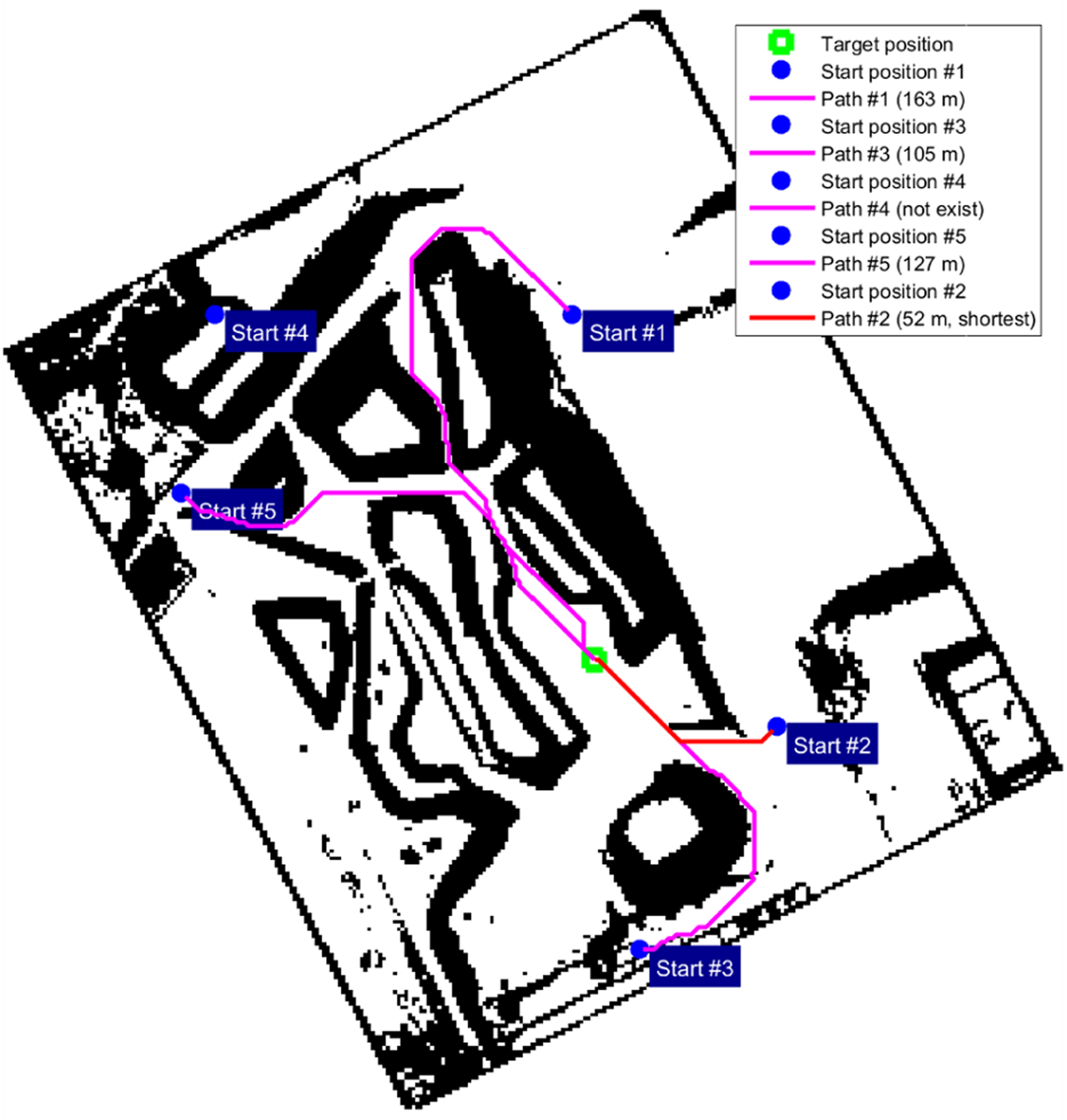
A binary obstacle map is obtained from the successfully formed DEM to retrieve the shortest path to the ROI. The slope threshold limit to mark a relevant cell in the map as an obstacle for the UGV is 15°. The cell size in the down-sampled obstacle map was set to 150% of the robot width, yielding a map with 300 × 285 pixels (0.9 m/pixel). Such a resolution allows us to find one path within seconds on a common PC unit. The possible mission starting positions were manually selected in the orthophoto map. The identified trajectories to the target spot are shown in Figures 17 and 18. The point at which the robot was unloaded from the car was chosen from among the starting positions offering the shortest paths (with the most advantageous one being 83-m-long). The final path was planned using the A* algorithm, and it ran between the unloading point and the first waypoint of the polygon where the mapping had been performed.

Figure 17.

The obstacle map with possible trajectories to the target.

Figure 18.

The orthophoto map with possible trajectories to the target.

Robot navigation accuracy

The robot navigation accuracy was determined as the waypoint tracking accuracy. The relevant value was estimated from the real trajectory of the mobile robot and the positions of the waypoints to be passed around. The error distance between the robot trajectory and a waypoint embodies the closest distance between a waypoint and the real robot trajectory, as demonstrated in Figure 19. The histogram of the error distance related to the waypoint tracking along the entire trajectory applied within the standard mapping method is presented in Figure 20. The error distances are evaluated on the horizontal plane (east–north). The average error equals 2.8 cm.

Figure 19.

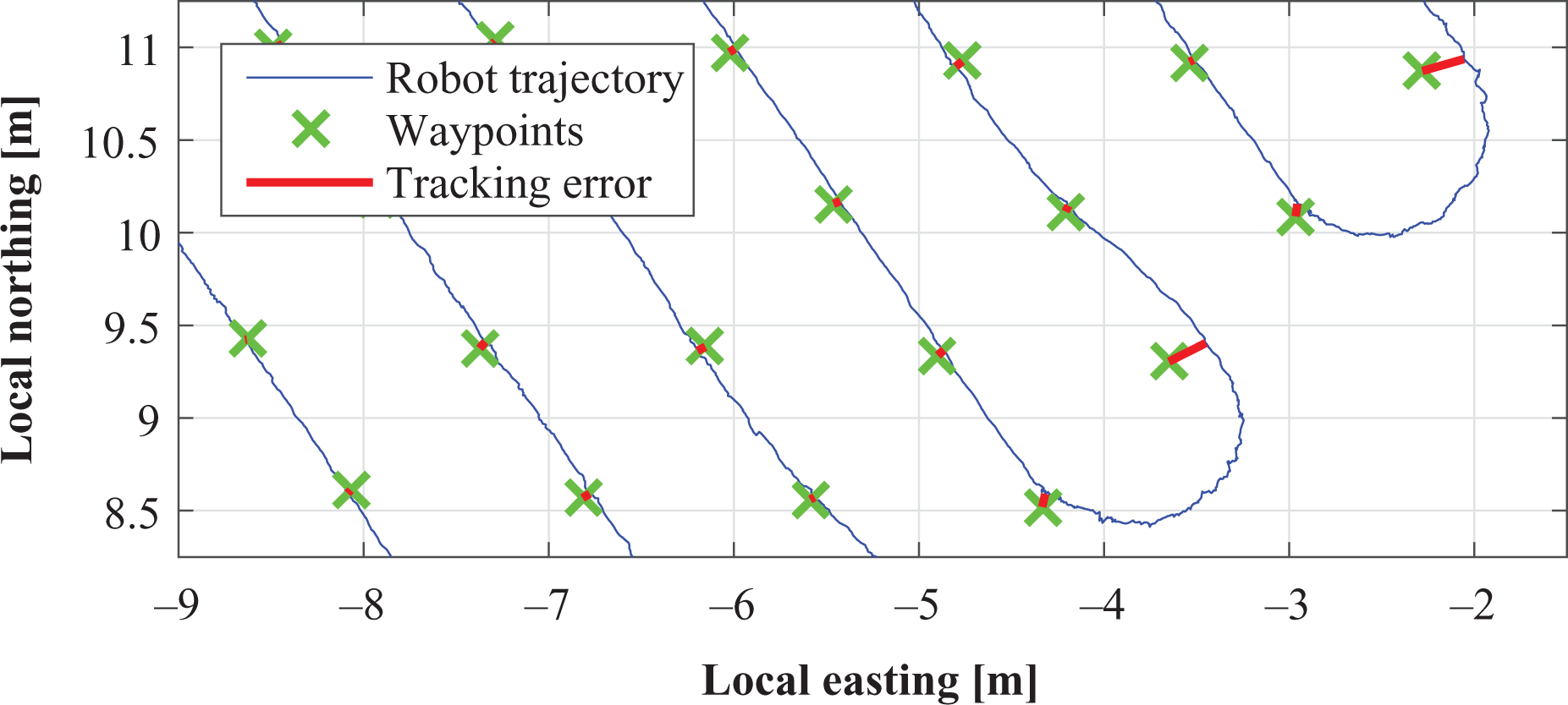
The errors in waypoint tracking on the trajectory.

Figure 20.

The errors in waypoint tracking on the trajectory.

Radiation sources localization

The proposed methods to localize gamma radiation sources were first simulated and then tested with actual radionuclides. There are two main reasons to run the simulations: (a) The behavior of the algorithm is influenced by several parameters to be set prior to any experiment, for example, the peak prominence and azimuth change constants; and (b) it is vital to set up the experiments in a manner that enables the algorithms to work as expected, meaning that when the experiments are prepared using simulation, the time needed on site can be reduced.

The radioactive decay of a source is a process describable with the Poisson distribution. The probability of the emission of x photons is expressed as²²

p (x = X) = P (x; λ) = \frac{e^{- λ} λ^{x}}{x!}

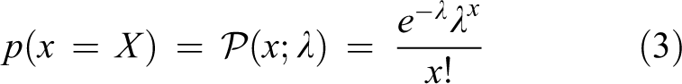
where λ denotes the mean emission of photons and its value is proportional to the source’s activity. On the short-term basis, this activity is approximately constant in the employed radionuclides. In the long-term run, it decays following the equation²²

A = A_{0} e^{- \frac{t}{T_{1 / 2} ln (2)}}

where T _1/2 is the half-time of the radionuclide, and A ₀ represents its original activity (usually stated in the calibration protocol).

Since the λ values are typically in the order of thousands and the Poisson distribution is numerically stable within the order of tens at most, the sources were approximately modeled using the normal distribution. The radiation background was modeled with the uniform distribution. The detectors were assumed to exhibit 100% conversion efficiency, and only their directional characteristics were considered. The dependence of the registered counts on the distance from a source is given by the inverse square law. Given the parameters of the sources, it is possible to calculate the counts registered in a measurement period by the detectors at any point. The total count detected by the detector k can be obtained from the following equation

C_{k} = c_{B} + \sum_{r = 1}^{R} c_{k, r}

where $c_{B} \leftarrow U ([c_{B, min}; c_{B, max}])$ is the contribution of the background, and c_k,r denotes the count rate due to the source r. The relevant value is given as

c_{k, r} = \frac{K_{k} (φ_{k, r}) a_{r}}{| | x_{k} - x_{r} {| |}^{2} + h_{k}^{2}}

where K_k (φ) is the sensitivity in the direction φ, φ_k,r is the angular coordinate of the source r in the coordinate system of the detector k, $a_{r} \leftarrow P (λ_{r})$ stands for the number of emitted photons, x _k and x _r are the coordinates of the detector and the source, respectively, and h_k is the height of the detector k above the ground. The simulations were run for multiple values of each parameter within the relevant possible range, with the parameter values set according to a convenient optimality criterion.

The radionuclides used for the experimenting are summarized in Table 4, together with their actual activities. All the experiments took place in the same polygon that had been defined using the map acquired by the UAV. The positions of the sources were measured prior to the experiments in order to provide the reference data.

Table 4.

The parameters of the radionuclides.

Label	Radionuclide	Activity (MBq)
S ₁	⁶⁰Co	8.0
S ₂	⁶⁰Co	40.0
S ₃	¹³⁷Cs	65.6
S ₄	¹³⁷Cs	0.22
S ₅	⁶⁰Co	0.35

To test the mapping algorithm, sources S ₁, S ₄, and S ₅ were placed in the ROI, with the spacing sufficient to facilitate their differentiation. The distance between the parallel lines was set to 1 m. The data acquisition took 15 min and 3 s. The map resulting from the application of a Delaunay triangulation is shown in Figure 21, where the black crosses mark the positions of the sources gained through the interpolation. The mean error of the computed positions corresponded to 0.06 m.

Figure 21.

The result of the mapping algorithm.

The next algorithm, strong source search, was tested using source S ₃. After the passage of the first two lines, we localized the direction in which the source had been estimated. The whole localization process lasted 2 min and 53 s, including the final loop around the source. The resulting trajectory consisting of data points is visualized in Figure 22. The achieved position error equals 0.04 m (the same order as in the mapping). The experiment was repeated using source S ₂, where the achieved error corresponded to 0.94 m. Since the azimuth was not corrected while approaching the source, the result strongly depended on the accuracy of the initial estimation.

Figure 22.

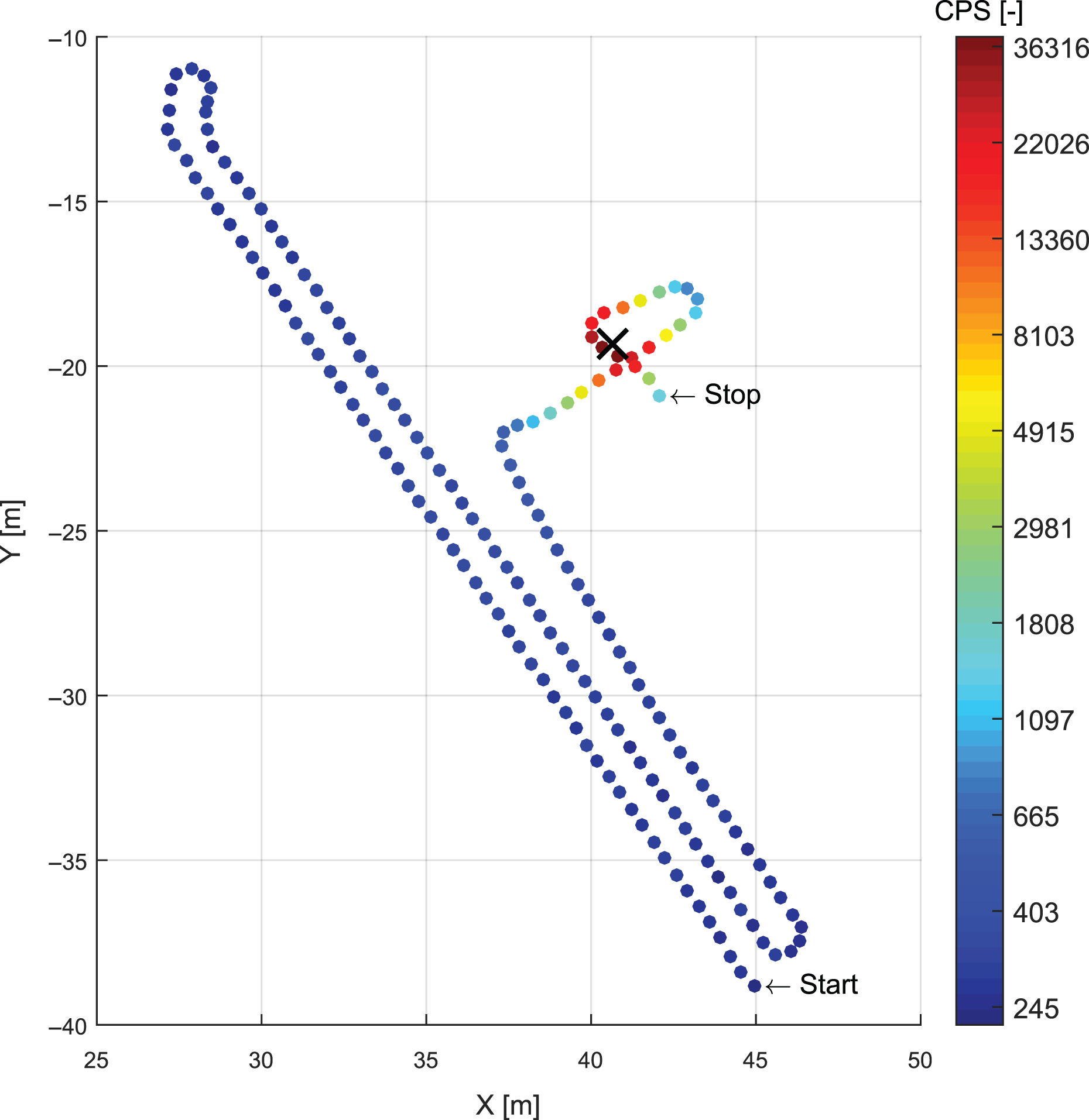
The result obtained with the strong source search algorithm.

First of all, the circular algorithm was verified with one source (S ₂); the source was located after 1 min and 28 s, with the position error of 0.52 m. After the actual completion, another experiment was set up, using two sources (S ₁ and S ₂) placed inside the area in such a manner that the circular trajectory lay between them. The resulting trajectory can be seen in Figure 23; apparently, the initial estimation of the direction in which source S ₂ can be found is rather inaccurate. However, thanks to the proposed continuous correction of the azimuth, both the sources were eventually located, and the mean position error corresponded to 0.40 m. The entire experiment took 2 min and 54 s.

Figure 23.

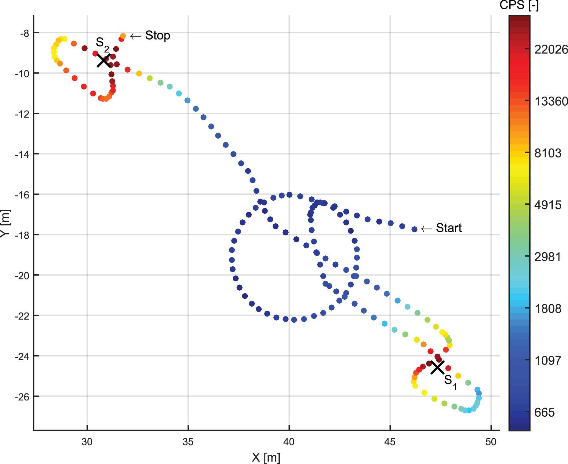
The result achieved via the circular algorithm.

Discussion

The UAV has proven to embody a very effective tool for fast and accurate aerial mapping. The presented custom-built multi-sensor system to facilitate DG can be carried by any UAV that exhibits a sufficient payload capacity, thus enabling the actual photogrammetry to be performed without using GCPs. This is essential when mapping areas are inaccessible or dangerous to humans, including, for example, those characteristic of natural disasters or radiation mapping. The elimination of GCPs also allows us to automate the entire mapping process, resulting in no need of human interaction during the data acquisition processing.

The spatial ground accuracy of the multi-sensor system related to the above flight mission is 4.1-cm RMS, a sufficient accuracy rate for UGV navigation. This is a result surpassing those achieved within similar projects. Turner et al.²³ obtained the spatial accuracy of 11 cm using a multicopter carrying a digital single-lens reflex camera (Canon EOS 550D, Tokyo, Japan) synchronized with a positioning system based on a differential global positioning system (GPS) receiver. Fazeli et al.²⁴ then used a low-cost RTK GPS module to perform DG; however, they generated a spatial error of 29-cm RMS due to inaccurate time synchronization. A system similar to the one presented in this research report is characterized in a related paper by Eling et al.,²⁵ who also used a multicopter UAV equipped with a dual antenna RTK GPS receiver, paying special attention to the calibration and time synchronization. The experiment yielded very accurate results, namely, 1.4-cm RMS for the XYZ axes, but these were achieved with a very low altitude and flight speed (20-m AGL, 2 m/s).

If we compare the accuracies of DG with those of IG, the former are typically slightly worse but remain comparable in selected cases. The object accuracy of a model georeferenced using IG mainly depends on the quality of the ground markers (GCPs), but it also reflects the flight altitude and ground resolution. The spatial error of the IG technique is normally within centimeters, as presented in, for example, the corresponding papers by Fazeli et al.,²⁴ Barry and Coakley,²⁶ and Panayotov.²⁷ But, as already mentioned, this approach is not suitable for our application due to the need of ground markers.

In the present article, the UAV was employed for optical mapping only; nevertheless, if a higher payload capacity was available, a detector of ionizing radiation could also be carried. In such a case, the orthophoto would be expanded to include the radiation intensity layer an outcome very beneficial for localizing the ROI. Yet this type of radiation maps cannot be as accurate and detailed as that produced by ground mapping (UGVs), because a typical flight altitude of a UAV is within tens of meters AGL. Ionizing radiation mapping via UAV is discussed in, for example, papers by Kaiser et al.,¹² Torii and Sanada,²⁸ or Martin et al.²⁹

Since the UGV does not possess the ability to avoid obstacles autonomously, the DEM is a valuable aid for the operator to define the region where the UGV can operate safely.

In this article, three different strategies to survey the ROI are introduced and tested in real conditions. The basic surveying method consists in a mapping algorithm which provides reference of the time costs and localization accuracy for the other algorithms. Mapping the selected ROI with the area of 438 m² took approximately 15 min, with the line spacing corresponding to 1 m. Since the trajectory was planned evenly inside the ROI, the dependence of the time intensity on the region’s area is rather linear. This fact embodies the major disadvantage of the mapping: the given operating time of the UGV equaled 120 min, and the maximum region that can be surveyed within a single action is limited to an area of roughly 3500 m². Conversely, the advantages include the ability to negotiate radiation hotspots other than isotropic point sources—for example, area or directional sources (such as a radionuclide in an open lead container). Both the sensitivity and the accuracy of the method may be increased by setting smaller line spacing and lower forward speed of the robot; the survey, however, is then likely to be more time-consuming.

The methods based on a dynamic change of the trajectory in accordance with the information provided by the detectors reduce the time consumption while ensuring a similar accuracy. Together with the time-saving feature, the strong source search algorithm provides two considerable benefits: First, if no source is found or present, the operator still gains the data allowing them to reconstruct the radiation map; second, the method is independent from the applied detection system and thus can be employed with other types of detectors, even the non-spectrometric ones. A disadvantage rests in the marked dependence of the result on the position of the source with respect to the initial position of the robot.

The circular algorithm, however, remains unaffected by this drawback and was discussed in the present paper as an alternative to the strong source search algorithm, which can beneficially exploit a direction-sensitive detection system. The relevant experiment proved that, under certain conditions, more than one source is localizable. The central importance of the algorithm nevertheless consists in its being a fundamental block for a more advanced localization algorithm to explore larger areas. Considering sources detectable at the distance of 4 m (in the case of the detection system outlined in this article, such sources consist in radionuclides ⁶⁰Co or ¹³⁷Cs, showing activity in the order of tens of megabecquerels), one circle covers the area of approximately 200 m². Within the experiments, such a circular trajectory was completed during 48 s. But assuming the time consumption associated with the movement between the circles, a primary survey of the ROI chosen in this article would last roughly 2 min—a major reduction in the time cost compared to the mapping.

The mapping algorithm provides localization accuracy in the order of centimeters. Johsi et al.³ presented a helicopter-borne radiation detection system and discussed the localization of a source having an intensity similar to that exhibited by the sources in our experiments. The obtained localization accuracy is within the order of meters, embodying a result expectable with respect to the character of the method. More interesting, however, appears to be a comparison with the achievements of UGVs. Lin and Tzeng⁶ proposed a method for localizing a radiological source via a mobile robot; the technique exploits an artificial potential field and a particle filter which, respectively, can negotiate the obstacles and simplify the localization. The method was verified by means of a simulation only with one source, with the achieved estimation error amounting to 0.02 m. Ristic et al.⁷ then presented an information-driven source search method. The concept was tested using Monte Carlo simulations in a square area (100 × 100 m²) accommodating one source, with the results comprising an average search that took 90 s and yielded an accuracy in the order of tenths of meters. The relevant simulation cycles were verified using two data sets measured in real conditions. Although the method appears to be promising in terms of the time efficiency, it is still awaiting practical application. Other innovative surveying strategies were introduced by Cortez et al.,⁹ who nevertheless verified their research only in an area of 60 × 60 cm², insufficiently for the discussed scenarios. The localization accuracy of the method is limited to 4 cm. A rather different scheme is described by Duckworth et al.¹⁰; their source is localized inside a collapsed building, and the process strongly depends on the assistance from an operator. Eventually, it took a minute to localize the source inside a 6 × 6 m² space.

The results within the present article are outlined using counts per second values, because the detectors were not properly calibrated prior to the experiments. Regarding the pursued goal, namely, the localization of radiation hotspots, the information value of the count rate is sufficient. The human operator may decide on the severity of the situation by comparing the values measured inside the ROI and the background value acquired after the deployment of the UGV. As the measured spectra are stored, they can be later approximately converted to dosimetric quantities if desirable—for example, as information for the operative team charged with the elimination of the given risk.

Although the radiation map is acquirable via the UGV alone, there are several reasons for choosing the proposed cooperation with the UAV. The main advantage consists in the possibility of using the DEM, which allows the UGV to navigate between terrain obstacles and can be beneficial for the operative team as well. Furthermore, if the radiation layer is measured during the aerial data acquisition, the area to be searched by the UGV can be reduced to save time and energy. In general, the cooperative approach combines the advantages of UAV- and UGV-based solutions, minimizing the disadvantages related to the stand-alone operation of each of these systems.

Conclusion

This article outlined the process of localizing ionization radiation sources via cooperation between a UAV and a UGV. All the presented methods were duly implemented, and special attention was paid to verifying the theoretical assumptions via a real mission as many similar projects rely on simulated data only. A UAV equipped with a custom-built multi-sensor system was employed to acquire the aerial data, and since this system had been designed for DG, the technique does not require ground markers. The object accuracy obtained through photogrammetry corresponded to 4-cm RMS, and both an orthophoto and a DEM were used for the UGV trajectory planning.

An Orpheus-X3 UGV equipped with a purpose-designed gamma radiation detection system was used to test several strategies facilitating radiation source localization. Regarding the general mapping method, the localization accuracy of 6 cm was achieved in the strong and weak sources placed simultaneously inside the selected ROI. Subsequently, an information-driven method based on the data acquired by an omnidirectional detector was designed and tested, enabling us to localize a single source at a rate of approximately five times faster than that achievable with the mapping algorithm. Furthermore, a pair of radiation detectors were utilized to assemble a detection system with considerable directional sensitivity. A modified algorithm exploiting such sensitivity, however, may ensure even better time efficiency; under certain conditions, the method allows us to localize a single source 10 times faster than the basic method. When confronted with the common approaches in terms of the localization accuracy, the improved procedure performs worse by an order of magnitude; yet the resulting information suffices for neutralizing a source. Figure 24 illustrates the composition of both the aerial and the ground mapping processes.

Figure 24.

Georeferenced map containing orthophoto layer with hill shading created using UAV photogrammetry complemented by the gama radiation intensity layer created by UGV. UAV: unmanned aerial vehicle; UGV: unmanned ground vehicle.

In the future, UAVs equipped with gamma detectors will likely be usable in rough radiation mapping, allowing the automatic detection of ROIs. This, along with implementing obstacle avoidance in UGVs, would lead to the more autonomous localization of radiation sources.

Footnotes

Declaration of conflicting interests

The author(s) declared no potential conflicts of interest with respect to the research, authorship, and/or publication of this article.

Funding

The author(s) disclosed receipt of the following financial support for the research, authorship, and/or publication of this article: This work was supported by the European Regional Development Fund under the project Robotics 4 Industry 4.0 (reg. no. CZ.02.1.01/0.0/0.0/15_003/0000470).

Appendix

References

Radiological Dispersal Device Playbook. Public health emergency. Washington, DC: US Department of Health and Human Services, 2015.

Ferguson

Kazi

Perera

. Commercial radioactive sources: surveying the security risks. Occasional paper No. 11. Monterey, California: Monterey Institute of International Studies, Center for Nonproliferation Studies, 2003.

Johsi

Quiter

Maltz

. Measurement of the energy-dependent angular response of the ARES detector system and application to aerial imaging. IEEE Trans Nucl Sci 2017; 64(7): 1754–1760. DOI: 10.1109/TNS.2017.2693988.

Hartman

Barzilov

Novikov

. Remote sensing of neutron and gamma radiation using aerial unmanned autonomous system. In: 2015 IEEE nuclear science symposium and medical imaging conference (NSS/MIC), San Diego, CA, USA, 31 October–7 November 2015, pp. 1–4. IEEE.

Aleotti

Micconi

Caselli

. Unmanned aerial vehicle equipped with spectroscopic CdZnTe detector for detection and identification of radiological and nuclear material. In: 2015 IEEE nuclear science symposium and medical imaging conference (NSS/MIC), San Diego, CA, USA, 31 October–7 November 2015, pp. 1–5. IEEE.

Lin

Tzeng

. Searching a radiological source by a mobile robot. In: 2015 international conference on fuzzy theory and its applications (iFUZZY), Yilan, Taiwan, 18–20 November 2015, pp. 1–5. IEEE.

Ristic

Morelande

Gunatilaka

. Information driven search for point sources of gamma radiation. Signal Proc 2010; 90(4): 1225–1239. DOI: 10.1016/j.sigpro.2009.10.006.

Wilde

Murphy

Shell

. A man-packable unmanned surface vehicle for radiation localization and forensics. In: 2015 IEEE international symposium on safety, security, and rescue robotics (SSRR), West Lafayette, IN, USA, 18–20 October 2015, pp. 1–6. IEEE.

Cortez

Papageorgiou

Tanner

. Smart radiation sensor management. IEEE Robot Autom Magaz 2008; 15(3): 85–93. DOI: 10.1109/MRA.2008.928590.

10.

Duckworth

Shrewsbury

Murphy

. Run the robot backward. In: 2013 IEEE international symposium on safety, security, and rescue robotics (SSRR), Linkoping, Sweden, 21–26 October 2013, pp. 1–6. IEEE.

11.

Martin

Payton

Fardoulisi

. The use of unmanned aerial systems for the mapping of legacy uranium mines. J Environ Radio 2015; 143: 135–140. DOI: 10.1016/j.jenvrad.2015.02.004.

12.

Kaiser

Darby

Matos

. UAV-based mobile gamma spectrometry. In: CTBT science and technology 2017 conference, 2017.

13.

Gabrlik

Jelinek

Janata

. Precise multi-sensor georeferencing system for micro UAVs. 14th IFAC Conf Program Device Embed Syst (PDES) 2016; 49(25): 170–175. DOI: 10.1016/j.ifacol.2016.12.029.

14.

Gabrlik

Cour-Harbo

Kalvodova

. Calibration and accuracy assessment in a direct georeferencing system for UAS photogrammetry. 2017, Manuscript submitted for publication.

15.

Jilek

. Advanced navigation in heterogeneous multi-robot systems in outdoor environment. PhD Thesis, Brno University of Technology, Czech Republic, 2015.

16.

Jilek

. Radiation intensity mapping in outdoor environments using a mobile robot with RTK GNSS. In: International conference on military technologies (ICMT) 2015, Brno, Czech Republic, 19–21 May 2015, pp. 1–7. IEEE.

17.

Hart

Nilsson

NJ,

Raphael

. A formal basis for the heuristic determination of minimum cost paths. IEEE Trans Syst Sci Cybern 1967; 4(2): 100–107. DOI: 10.1109/TSSC.1968.300136.

18.

Finkel

Bentley

. Quad trees a data structure for retrieval on composite keys. Acta Inform 1974; 4: 1. DOI: 10.1007/BF00288933.

19.

Harabor

Grastien

. The JPS pathfinding system. In: 26th national conference on artificial intelligence, 2012.

20.

Amidror

. Scattered data interpolation methods for electronic imaging systems: a survey. J Elect Imag 2002; 11(2): 157–176.

21.

Miller

Machrafi

Mohany

. Development of a semi-autonomous directional and spectroscopic radiation detection mobile platform. Radiat Meas 2015; 72: 53–59. DOI: 10.1016/j.radmeas.2014.11.009.

22.

Ahmed

. Physics and engineering of radiation detection. Amsterdam, The Netherlands: Elsevier Science Limited, 2007. ISBN: 978-0-12-045581-2.

23.

Turner

Lucieer

Wallace

. Direct georeferencing of ultrahigh-resolution UAV imagery. IEEE Trans Geosci Remote Sens 2014; 52(5): 2738–2745. DOI: 10.1109/TGRS.2013.2265295.

24.

Fazeli

Samadzadegan

Dadrasjavan

. Evaluation the potential of RTK-UAV for automatic point cloud generation in 3D rapid mapping. ISPRS Int Arch Photogram Remote Sens Spatial Inform Sci 2016; XLI(B6): 221–226. DOI: 10.5194/isprs-archives-XLI-B6-221-2016.

25.

Eling

Wieland

Hess

. Development and evaluation of a UAV based mapping system for remote sensing and surveying applications. ISPRS Int Arch Photogram Remote Sens Spatial Inform Sci 2015; XL-1(W4): 233–239. DOI: 10.5194/isprsarchives-XL-1-W4-233-2015.

26.

Barry

Coakley

. Field accuracy test of RPAS photogrammetry. ISPRS Int Arch Photogram Remote Sens Spatial Inform Sci 2013; XL-1(W2): 27–31. DOI: 10.5194/isprsarchives-XL-1-W2-27-2013.

27.

Panayotov

. Photogrammetric accuracy of real time kinematic enabled unmanned aerial vehicle systems. Study conducted by the University of Colorado, Denver and Juniper Unmanned Aerial Systems for the United States Geological Survey, Colorado, USA, 2015.

28.

Torii

Sanada

. Radiation measurement by unmanned aircraft after Fukushima Daiichi nuclear power plant accident: Remotely piloted aircraft systems symposium ICAO headquarters, Montreal, Canada, 2015.

29.