AirGuardian – UAV Hardware and Software System for Small Size UAVs

Abstract

AirGuardian is a complex of an Unmanned Aerial Vehicle and ground station UAV hardware and software systems which has been developed at Obuda University. The hardware and software of the autopilot (AERObot), the antenna tracker station and the ground control station were simultaneously created resulting in the optimal cooperation of the modules.

The aim of the research on AERObot – the special autopilot – was to create a generic autopilot which is capable of controlling different designs, weights and structures of airframes without any complex mathematical model recalculation.

1 Introduction

AirGuardian was created to meet these criteria: Antenna tracker unit

Compact unit without any other wired module • Automatic self-calibration before flight

Autonomous tracking of the UAV

Ground Control software connectivity

Ground control software

Multi-user server-client architecture with different capabilities (navigator, observer mission planner and pilot)

Full mission record and replay features

Support of custom-calibrated maps

AERObot (onboard hardware and software)

Compact, small size and low weight electronics, without wired off-board sensors

Module-based design with slot based architecture to achieve task specific application

Universal communication interface allowing the usage of both wireless (different RF modems) and wired (FTDI USB) connectability

Autopilot can store at least 200 waypoints, the parameters of planes and control functions in a non-volatile memory

Fully autonomous operation (telemetry issues should not affect the flight)

1.1 Antenna tracker unit and ground control station

The ground electronics of the system are in the antenna tracker unit. The main task of the unit is involves RF communication with the UAV using directed high gain antennas and the wired communication with the ground control PC.

The tracker unit (Fig. 1) also has an onboard GPS so it is not only able to track the UAV from a single position but so that it also possible to use it as a mobile ground station. The tracker unit has two degrees of freedom, with limitless rotation on the yaw angle [1].

Figure 1.

Antenna tracker

The software is highly scalable. It can be used as a multiple workstation with one dedicated server and multiple role-based clients or else in a single, low-cost notebook with an admin role. The AirGuardian can also record and replay missions in real time. Multiple 2D and 3D maps can be imported, enabling multilayer maps and 3D satellite image-based mission planning.

1.2 Ground control software

The ground control software is based on client-server architecture. The server is connected to the antenna tracker, which grants the telemetry and camera data. It can handle serial ports or TCP/IP packets. Multiple clients can connect to the server from one or many PCs. The server also relays the telemetry to the Wi-Fi, allowing AirGuardian Mobile (smartphone version) to access mission data (Fig. 2).

Figure 2.

AirGurdian ground control software layout

The users are basically using the client software, communicating with the server through TCP/IP using wired or wireless networks. The users have authentication in the clients, which grants them the proper permissions (pilot, navigator, observer and admin roles). They can see the data related to their task only. For example, the pilot can control the UAV remotely using the front camera but they cannot modify autonomous mode waypoints or altitude as the navigator can. The client interface is customizable for each (new) role.

1.3 Onboard electronics

The onboard electronics have two modules for a general UAV application: the AERObot main board and the Servo board. The main board has all the units, with the exception of the IMU (inertial measurement unit), which are needed for autonomous flights. This means that only the IMU, the GPS antenna and the engine battery (for power consumption) is connected to the main board electronically. The other connectors are the static and dynamic pressure tubes from the Pitot-tube, which grants the airspeed and altitude parameters. Expander modules (e.g., the Servo panel) can be connected to the main board through two row headers. Additional electric sensors can be attached to the board (an ultrasonic altimeter, a revolution sensor, a temperature sensor, etc.), but these are not essential parts for a general UAV application.

Parameters of the AERObot 5.0 main board (Fig. 3):

Redundant power supply (with redundant 2–4S LiPo batteries)

Voltage sensing on batteries

GPS sensor with 10Hz update rate

Barometric altimeter with automatic calibration

Barometric airspeed meter with Pitot-tube

MicroSD memory card connector for data logging

Power consumption sensor up to 100A

6+2 channel PWM output for servo drive

Serial port for radio modem (telemetry and setup)

FTDI USB port (telemetry and setup)

Serial port for IMU (Both 3.3 and 5V with TTL or RS232 signal levels).

CAN bus

PWM input (ultrasonic altimeters or the revolution sensor)

Extender boards (e.g., the servo board or the sensor board)

External GPS port

3D waypoints (position, altitude, airspeed and actions)

Autonomous waypoint navigation

Full in-flight mission control (waypoints, parameters, controllers, etc.)

2 SPI channels

1 I2C channel

Figure 3.

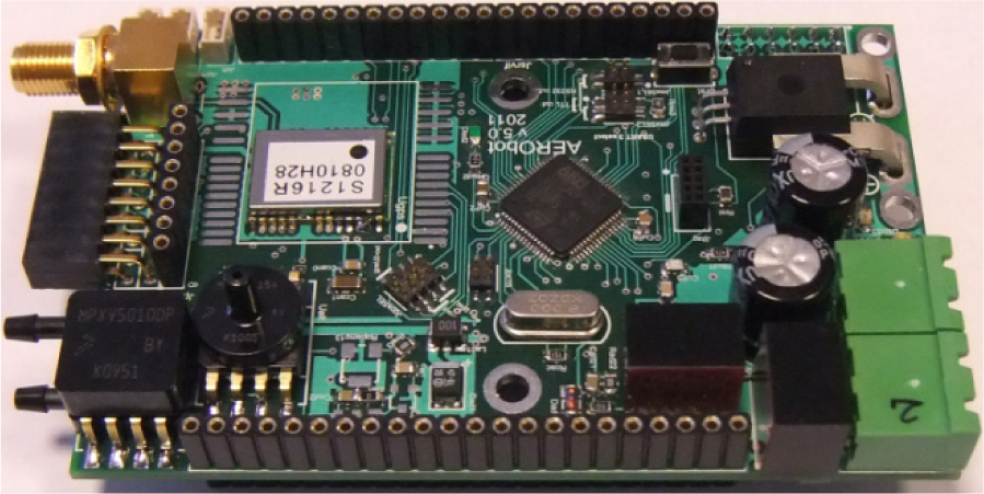
AERObot main board

The servo board was made as an interface to connect AERObot to a common radio control plane easily. The main function of the board is to relay the control signals created by the main board to the actuators of the plane. Furthermore, the sensor board can switch the controls between manual, heterogeneous and autonomous at circuit level without modifying the connections between the boards and the actuators.

This can be activated with an RC transmitter switch on a free channel or a with a telemetry command. For flight safety purposes, the board can handle two different RC receivers in diversity, which is important in manual control mode during the setup procedure. When the signal of a receiver is weak, the board automatically switches to the other receiver. When both lose signal, the board switches to autonomous stabilized flight.

Parameters of the AERObot Servo board (Fig. 4):

Dual receiver remote control

Autonomous, heterogeneous (8 preset autonomous-manual mixed control), manual mode

6+2 channel PWM output for the servo drive

1A onboard BEC for the low power actuators

High current BEC connector for external actuator power

Optional xBee, xStream and xTend radio modem connector with FTDI USB support

Modem and RC receiver RSSI sense

OSD (On Screen Display and character mode SPI controller).

Revolution meter input

4 switch relay output

4 ADC input.

Figure 4.

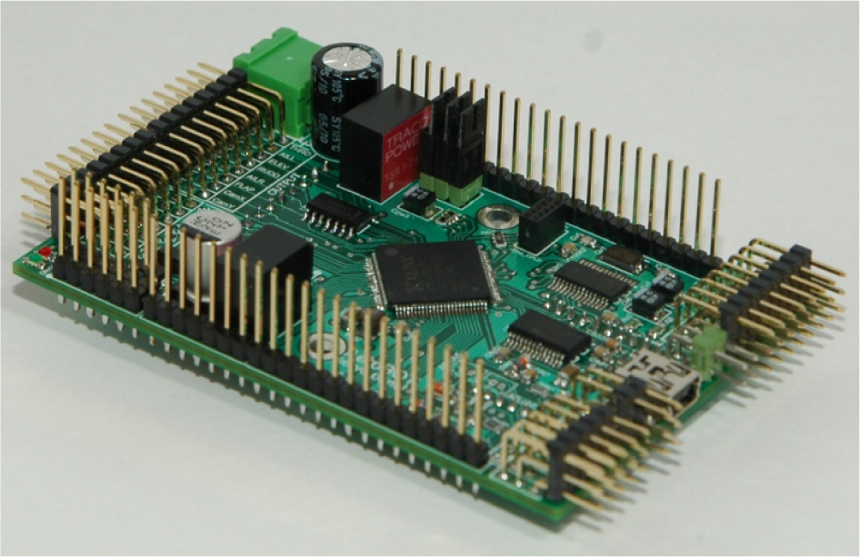
AERObot servo board

The two boards (main and servo) can control a general purpose UAV. Both the airplane and the payload can also be controlled (i.e., camera turn on/off, record, follow target, etc.). It is possible to attach further boards [2] to the main or servo board, such as the sensor board (analyse air composition, radiation, etc.), or else to further main boards (allowing redundant UAV control) (fig 5.).

Figure 5.

AERObot redundancy

AERObot saves all the parameters to a non-volatile memory, which means that after turning on the UAV and the GPS locks position, the system is then ready to use. The waypoints and mission directives can be set before the mission and can also be modified during flight.

2. AERObot waypoint navigation

There are many navigation approaches. Most of them use waypoints [3], defined by a geographic position (latitude and longitude), an altitude (above ground level or above sea level) and a waypoint radius (usually 25–75m is used to achieve precise path tracking). A waypoint is reached, when the distance between the UAV and the waypoint is under the predefined radius value. For precision navigation, the autopilot needs very accurate position and bearing information.

2.1 Bearing estimation

The base sensor for navigation is the GPS. This provides the position, the speed over ground (SOG), the bearing and many other parameters used by the navigation algorithms. The maximum position refresh rate of the best GPS modules is about 5–10Hz, which is not enough for precision flight control.

The other problem is that the refresh rate is not reliable because the NMEA sentences and the checksums are often incorrect. It is necessary to estimate the missing and intermediate positions for the continuous bearing control (100Hz – update frequency of the most commercial RC actuators). This estimation can be computed using the yaw rate and the GPS bearing from the last valid NMEA sentence. The Z-axis angular rate (provided by the IMU) should be converted to the heading turn rate using the UAV bank angle [4]. With this procedure, the actual bearing can be estimated between two valid GPS sentences (1). The heading angle provided by the IMU is often unreliable because of the magnetic sensor used by the internal sensor fusion algorithms. This sensor is very sensitive to strong electromagnetic fields, especially when the UAV has electric propulsion.

${\theta }_e=\mathrm{ }\theta +\mathrm{ }\dot{\Psi }\mathrm{ }$

(1)

where:

θ:previous bearing (measured by GPS), θe:estimated bearing, $\dot{\Psi }$ : heading turn rate.

Small sized (around 1 m wingspan) and low weight (under 2 kg) UAVs are quite agile and so turn rates can reach high levels. For these airframes, bearing estimation is essential (fig 6.).

Figure 6.

Flight test: the purple triangle indicates the estimated bearing

2.2 Position estimation

During navigation, both the bearing and the position have to be estimated with a navigation formula (2), which is well known in nautical terms [5]. The aim is not for a complete inertial navigation system with minimal error but rather the computation of intermediate positions and bearings in order to achieve better performance. As such, some things can be ignored [6, 7, 8].

$\begin{array}{l}{Lat}_2=\mathrm{asin}(\sin \left({Lat}_1\right)\mathrm{*}\cos \left(\frac{d}{R}\right)+\cos \left({Lat}_1\right)\mathrm{*}\sin \left(\frac{d}{R}\right)\mathrm{*}\cos \left({\theta }_e\right))\\ \begin{array}{c}{Lon}_2={Lon}_1+\mathrm{ }atan2(\sin \left({\theta }_e\right)\mathrm{*}\sin \left(\frac{d}{R}\right)\mathrm{*}\cos \left({Lat}_1\right),\cos \left(\frac{d}{R}\right)-\\ \sin \left({Lat}_1\right)\mathrm{*}\mathrm{s}\mathrm{i}\mathrm{n}\left({Lat}_2\right)\mathrm{ }\end{array}\end{array}$

(2)

where:

Lat1:previous estimated latitude of the UAV,

Lon1:previous estimated longitude of the UAV,

θ_e:estimated bearing (in radians, clockwise from north),

d: distance travelled,

R: The Earth's radius.

Usually, there are 200ms between two valid GPS sentence bursts, but the distribution of the measured positions is not uniform. Even if one or two is corrupted, the refresh time is always under 1000ms. Because of this, the direction and velocity of the wind can be ignored. During the estimation, the last known SOG can be used no matter how the bearing of the UAV changed (compared to the wind). Obviously, there will be some errors, but usually it is low (under 1m) and will not cause any serious false position estimation.

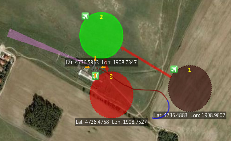
The estimation (Fig. 7) can be calculated from the previous known SOG, estimated position and bearing (when the known position and bearing are unavailable).

Figure 7.

Position estimation simulation from telemetry data (downsampled, the big dots are the measured positions and the small dots are the estimated positions)

The vector field navigation calculates a desired bearing in every position, no matter what the actual bearing of the UAV is. This can be easily represented as a vector field. The desired bearing depends on the position of the UAV, the source and destination waypoints and the cross track error (3).

$\begin{array}{c}\delta =\sqrt[K_d]{\left|D_{CT}\mathrm{*}{K}_c\mathrm{*}\left({\phi }_T-{\phi }_R\right)\right|}\mathrm{*}sign\left(D_{CT}\right)\\ \gamma =min\left(1,\mathrm{ }{D}_T\right)\\ {\phi }_d=\mathrm{ }{\phi }_T+\delta \mathrm{*}\gamma \mathrm{ }\end{array}$

(3)

where:

DCT: Cross track error,

φ_d: Desired bearing,

φ^T: Bearing from the UAV to the destination waypoint,

Kd: Path reaching smoothness parameter,

Kc: Cross track error sensitivity parameter,

γ: Waypoint bearing sensitivity parameter.

The cross track error sensitivity can be set with Kc parameter (Fig. 8) and the path reaching smoothness (Fig. 9) with Kd. It is a common problem that a UAV will miss the waypoint if the waypoint radius is low and there is a strong wind or else the distance between the source and the destination points is short. In this case, the UAV should turn back and the flight path will contain unnecessary loops. The first possibility for avoiding this problem is the dynamic radius which must suit local airflow characteristics.

Figure 8.

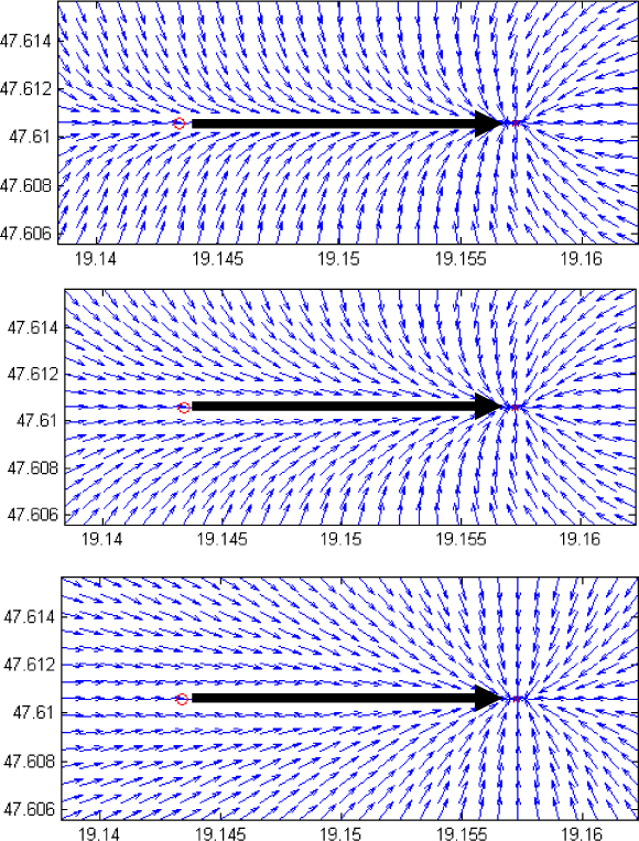
Effect of Kc with different values (10, 1, 0)

Figure 9.

Effect of Kd with different values (1, 0.5, 0.3)

The alternative – and better – solution makes use of γ. If the UAV is close to the destination point (under 1000m), the parameter γ guarantees arrival at the waypoint, ignoring δ depending upon the UAV – waypoint distance (Fig. 10).

Figure 10.

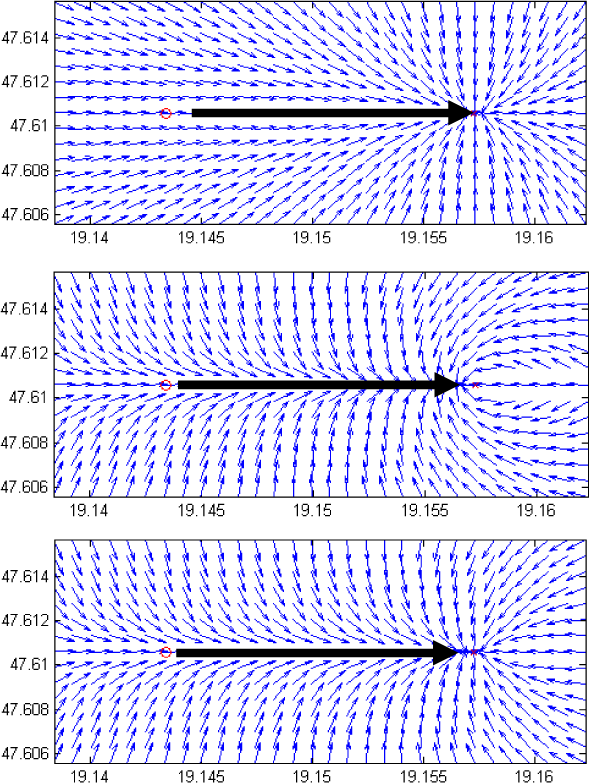
Effect of y with different values (0, 1, min(l, D_T))))

The first advantage of this form of navigation is the accessible graphical setup of the internal parameters Kc (∼10.0) and Kd (∼0.5). The other is that it has only one output parameter (φ_d) and so nearly any controller type (such as third-order nonlinear, PID, fuzzy, etc.) can fit this navigation because only one value – the difference between the desired and actual bearing – should be minimized. Furthermore, and with a little modification (4), it is capable of loiter navigation over a desired position (Fig. 11). This function is quite useful when the UAV is observing a destination position with a stabilized electro-optical or thermal imaging camera.

${\phi }_d={\phi }_T+\mathrm{ }\frac{\pi }{2}+min\left({|D}_{CT}\mathrm{*}{K}_c|,\frac{\pi }{2}\right)\mathrm{*}sign\left(D_{CT}\right)$

(4)

Figure 11.

Loiter navigation

where:

D_CT: Cross track error (distance from the radius),

φ_d: Desired bearing,

φ_T: Bearing from the UAV to the destination waypoint,

Kc: Cross track error sensitivity parameter.

3. Flying wing extension

Flying wings has no vertical or horizontal control surfaces – only elevons, which are a mix of elevator and rudder. This means that flying wings generally have no control along the vertical axis. However, some approaches exist to achieve vertical control. These are the so-called “drag rudders”, which are usually represented by asymmetric operated airplane dive brakes, such as Schempp–Hirth or the trailing edge brakes used on Horten 229 and Northrop YB-35.

The drag rudder approach used by AERObot is based on a conventional model glider brake system – the “butterfly” (Fig. 12) – which does not need any further mechanical control surfaces or actuators, using only the four control surfaces on the main wing. The inner two control surfaces (the flaps) are open down around 45–80°, while the outers (the ailerons) are open up by 5–45°, with a little elevator compensation on the tail. Based on the butterfly brake, a new drag rudder was developed (fig. 13, 14, 15). On the wing, there are four control surfaces – the inners are the elevators, the outers are the ailerons – which are all set to +3–4 mm up, as is usual on flying wings.

Figure 12.

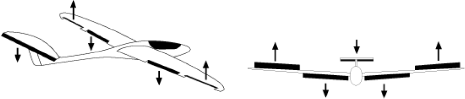
Butterfly brake on a model glider

Figure 13.

Ailerons on a flying wing from behind (left roll, straight flight, right roll)

Figure 14.

Elevators on a flying wing from behind (nose up, straight flight, nose down)

Figure 15.

Drag rudder on a flying wing from behind (left turn, straight flight, right turn)

On turns, the elevator moves up by 100%, the elevator down by 50% of the rudder command on the desired side (5).

$\begin{array}{c}{D}_L\left\{\begin{array}{c}1, if {\phi }_{RuddCMD}<0\\ 0, otherwise\end{array}\right.\\ D_R\left\{\begin{array}{c}1, if {\phi }_{RuddCMD}>0\\ 0, otherwise\end{array}\right.\\ {\phi }_{EleL}:\mathrm{ }{\phi }_{EleCMD}-\mathrm{ }\frac{{\phi }_{RuddCMD}}{2}\mathrm{*}{D}_L\\ {\phi }_{EleR}:\mathrm{ }-{\phi }_{EleCMD}-\mathrm{ }\frac{{\phi }_{RuddCMD}}{2}\mathrm{ }\mathrm{*}{D}_R\\ {\phi }_{AilL}:\mathrm{ }{\phi }_{AilCMD}+\mathrm{ }{\phi }_{RuddCMD}\mathrm{ }\mathrm{*}{D}_L\\ {\phi }_{AilR}:\mathrm{ }{\phi }_{AilCMD}+\mathrm{ }{\phi }_{RuddCMD}\mathrm{ }\mathrm{*}{D}_R\end{array}$

where:

φ_EleL: Left side elevator control surface deflection

φ_EleR: Right side elevator control surface deflection

φ_AilL: Left side aileron control surface deflection

φ_AilR: Right side aileron control surface deflection

φ_AilCMD: Aileron deflection command

φ_EleCMD: Elevator deflection command

φ_RuddCMD: Rudder deflection command

4. Experiences of the AirGuardian system

The setup procedure for a new plane is always begun with a manual test flight so as to examine the flight abilities and preset the control surfaces. Next, the control surface idle positions for the autopilot must be adjusted. The control loops must be set up independently first and then fine tuned during flight.

Fig. 16 represents an altitude plot of the first test flight of Chelidon UAV. It contains a manual take-off and multiple heterogeneous/autonomous flights. The red parts are manual control. In the early stage of the flight, the independent tuning of the control loops was made through the AirGuardian ground control software. During this period, the UAV was flown in heterogeneous mode 6 times. After the independent tuning, there were 4 autonomous flights when the combined control loop fine tunings were made. The first three flights were short, because the controllers were not well-tuned. The last autonomous part was a successful fine tuned flight, with many laps on a three waypoint route (Fig. 17). The whole procedure took 30 minutes.

Figure 16.

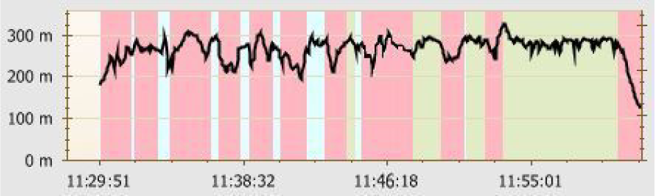
Altitude diagram – Chelidon first test flight (red: manual, white: heterogeneous, green: autonomous flight)

Figure 17.

Chelidon flight route in the AirGuardian Navigator view (partial)

This short time is remarkable since Chelidon was a brand new custom built prototype airplane, and so no preliminary flight data was available. The experiment confirmed that AERObot is robust and that the setup procedure is quick and effective.

5. Conclusions

Various experiments proved that AirGuardian met the criteria targeted at the beginning of the research. The onboard electronics and redundant systems were working reliably. The switch between manual, heterogeneous and autonomous is less faulty and transient.

The antenna tracker is capable of tracking the UAV in real time. After the GPS lock, it automatically turns to the UAV and starts following it. In case of telemetry loss, the antenna turret can be controlled manually for the plane with a remote.

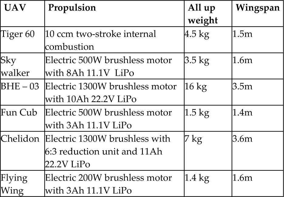
The UAVs used to test AERObot and AirGuardian are in Table 1. The examination displayed the abilities of the system using multiple, different sized and shaped UAVs. Comprehensive ground control software was developed which can effectively serve the UAV and the ground personnel. It can be used as a single or as a multiple workstation or even as a mobile application (fig 18.).

Table 1.

UAVs applied with AERObot and tested with AirGuardian system

UAVQ	Propulsion	All up weight	Wingspan
Tiger 60	10 ccm two-stroke internal combustion	4.5 kg	1.5m
Sky walker	Electric 500W brushless motor with 8Ah 11.1V LiPo	3.5 kg	1.6m
BHE – 03	Electric 1300W brushless motor with 10Ah 22.2V LiPo	16 kg	3.5m
Fun Cub	Electric 500W brushless motor with 3Ah 11.1V LiPo	1.5 kg	1.4m
Chelidon	Electric 1300W brushless with 6:3 reduction unit and 11Ah 22.2V LiPo	7 kg	3.6m
Flying Wing	Electric 200W brushless motor with 3Ah 11.1V LiPo	1.4 kg	1.6m

Figure 18.

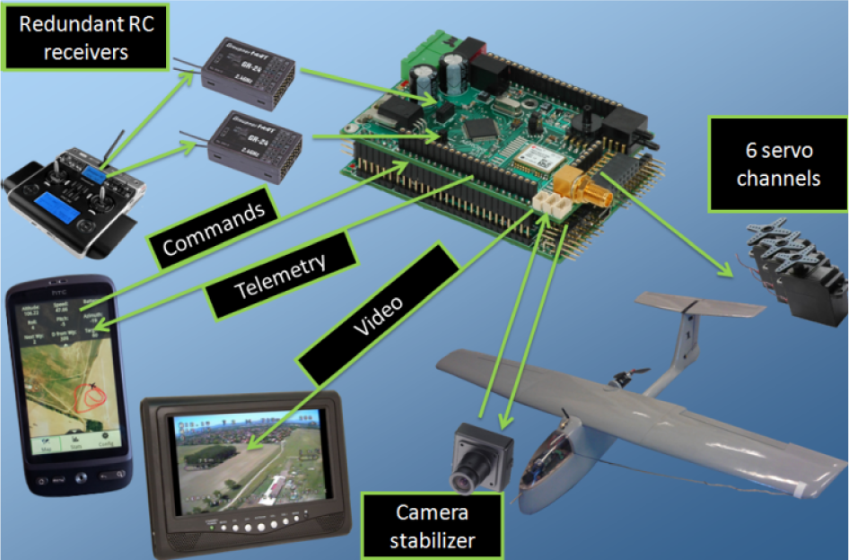
Complete AirGuardian system

As a result, the various parts of the system can be used as standalone units – e.g., an extension module to another existing system or as a part of a whole new development.