Sage Journals: Discover world-class research

Abstract

The objective of this article is to propose data processing from laser range finder that will provide simple, fast, and reliable object recognition including moving objects. The whole method is based on four steps: segmentation, simplification, correspondence between consequent measurements, and object classification. Segmentation uses raw data from laser range finder and it is significant in logical connection of related segments. The most important step is simplification which provides data reduction and acceleration of object classification. The output of simplification is an object represented by significant points. Correspondence between consequent measurements is based on kd-tree nearest neighborhood search. The object is then classified by its spatial changes. These changes are evaluated by position of correspondent significant points. Input of proposed procedure is a probabilistic model of laser range finder. In this article, versatile probabilistic model of Hokuyo URM-30 LX was used. The method was verified by simulations and by tests in real environment. The results show that proposed method is reliable and with small modifications (of parameters), it is usable with any other planar laser range finder.

Keywords

Laser range finder segmentation data points moving obstacles data pairing

Introduction

Common mobile robots work in environments, which are not separated from humans. This means they need to be able to detect not only static parts of environments but they also need to react to the moving obstacles, for example, different moving objects such as robots, humans, doors, and so on. That is why they need to scan this environment with powerful and reliable sensors, which can provide sufficient amount of data.¹ A laser range finder (LRF) is a commonly used example of such sensor. The development of LRFs begun at the end of the 60s, but their widespread use was only enabled by the fast integrated circuits. Due to continual decrease in price, they are already being used in hobby robotics or in domestic service robots.²

Research in sensorial elements is focused on three-dimensional (3-D) sensing of the environment. The first RedGreenBlue-Depth (RGB-D) cameras have already appeared on the market, which make them easily accessible for the wide public.³ However, they lack the necessary parameters for the navigation of robots in a dynamically changing environment. On the contrary, the high price of 3-D LRFs puts severe limitations on the number and the type of applications it can be used in. 3-D LRF can be constructed as a rotating two-dimensional (2-D) version; however, this solution is limited by its mechanical speed and thus can effectively only be used for the mapping of environment in static positions of the robot.⁴ For these reasons primarily, 2-D LRFs are used in the robot navigation in dynamically changing environment.

When working with LRF, it is necessary to know sensor’s measurement principles and properties. They are as follows^5,6:

triangulation,

time of flight,

frequency modulation continuous wave, and

phase shift measurement.

These measurement principles are well known and can be found and discussed in detail by Konolige et al.² or Nejad and Olyaee.⁵ However, the measurements of each LRF type are corrupted by various errors. Therefore, models were devised for accurate data interpretation.^{7

–19}

Segmentation and feature detection in LRF data is used in various tasks, for example, detection of moving obstacles. Segmentation is the fundamental element of data processing. Its aim is to divide the measurements into parts, which represent a consistent segment of the measured space—that is, an object. As for LRF measurements, the majority of objects are described by several measurements (data points). Based on this, their shape can be estimated and the amount of recorded data may be reduced. The results of such algorithms are usually segments, which are composed of data points or characteristic features.

Often, segmentation is based on the distance between the data points. This segmentation compares two subsequent data points from the LRF measurements. If their distance is greater than the threshold, the measurement is divided into two segments at this border.¹⁸ The threshold is usually determined as a constant or it is adapted to the measurements.²⁰ This adjustment of threshold can be based on the shape^18,21 or on the orientation of the detected obstacles.²²

The segmentation of LRF data can also be based on the straight line searching. These algorithms are sequential and they evaluate whether a data point belongs to the previous segment or it is a new one. This evaluation is also based on the threshold. Each straight line is created from two points. If the evaluated point belongs to the previous segment, this point will be the new end point of the line segment. Otherwise, a new line segment is added. The advantage of this algorithm is that it is easily applicable in polar coordinates.^23,24 Similar principle is used in the algorithm of line tracking.²⁵ This method can be used with other geometrical shapes, which can be described by the analytical geometry.¹⁸

Segmentation based on lines can also be performed by recursive algorithms.^23,24,26 These algorithms search for the segments on the whole data set from LRF. If there is a point, which does not fulfill the criterion, the data set is divided into two subsets. The algorithm consequently performs the procedure on both subsets. This is done until all the points from the data set fulfill the criterion. Usually, the criterion is based on thresholds like in the previous algorithms. Norouzi et al.²⁷ proposed modification with Hough transformation. Hough transformation divided the data points into nearby segments—rough approximation of linear segments. Recursive algorithm is afterward applied on each nearby segment.

Split and merge algorithms divide the data points into individual lines. This first step may be performed by sequential algorithms,²⁵ recursive algorithms,^26,28,29 or by extended Kalman filtering (EKF).³⁰ The second step consists of line merging. Only lines with similar parameters are merged.

Significant shapes (segment) in the data points can be searched by Local Curvature Scale.³¹ This algorithm determines the rate of curvature for each data point. Rate is expressed as neighborhood where the segment does not change the shape significantly. If the rate is higher, the segment can be considered as line segment.³² Similar principle is used in the curvature function. In this method, the rate of curvature is determined from direction derivatives and it is expressed in degrees. Corners are then local maximums and straight segments are evaluated by values near to 0. This method also enables the detection of rounded objects.³³

LRF measures the distances in polar coordinates and the majority of mentioned methods work in Cartesian coordinates.³⁴ Therefore, it is often necessary to perform additional calculations. However, the measurements in polar coordinates can be considered as distance histogram, that is, one-dimensional (1-D) curve. Searching in such 1-D space significantly reduces the computational complexity. This is applied in gradient search algorithm in polar coordinates.³⁵ Basic assumption of this algorithm is that the significant features are located where there is a change of the measured distance. In these points, the gradient crosses zero.

The segmentation of data points from LRF measurements is the basic assumption of each algorithm used for the detection of moving obstacles. The identification of moving obstacle usually involves the pairing of segments from two consecutive data points and looking for the changes in the position of each segment with respect to the own robot’s motion. Segments representing the objects in the environment can be described as follows:

occupancy grid,^36

–39

geometrical shape,^40
–42

significant features,^21,41,43,44and

point cloud.^45,46

Each of these representations has its own advantages and the correspondence searching (pairing of segments) is based on it. Generally, the majority of mentioned methods are based on some type of distance searching (Euclidean and Mahalanobis³⁶) or on the object similarity. The largest source of error is the coverage of moving objects, sudden changes in the shapes of objects between two consequent measurements, and the position error of the robot.

If the correspondence between two segments is found, then it is possible to determine whether the object is moving or static. For this purpose, it is possible to use simple regressive methods based on EKF⁴⁷ or particle filter.⁴⁸ Advanced methods work with the information about the object’s type.

The detection of moving obstacles in the occupancy grid requires the modification of occupancy grid itself. One option is to create the new occupancy grid for each measurement and the detection of moving obstacles can be performed by image processing algorithms, such as optical flow.³⁷ The disadvantage of these algorithms is that they also process the places in the occupancy grid with no object present. Therefore, these methods require extensive computing power. Another option is the extension of occupancy grid with the information, when the cell was changed last time. This can help to determine, if the new measurement is a moving obstacle.³⁶ Another modification of occupancy grid divides it into two grids—static and dynamic.³⁸ Extending this algorithm onto several occupancy grids, each containing information about a single moving object, may lead to the acquisition of accurate information about individual objects.^45,49

All objects measured by LRF can be represented by basic geometrical shapes. The advantage of this representation is the possibility to use analytical geometry to determine the distance and similarity between two objects.^41,42 The disadvantage of these algorithms is the loss of information about the real shape of the objects, which is why the information about similarity of two objects has low information value. Objects can also be described by convex hull, which better reflects the shape of the object.⁴⁰

The detection of moving obstacles based on significant features requires at least one significant feature on each object. These features can be characterized as edges,⁴³ points,²¹ or combined features as corners (two edges and one point).⁴¹ The significant feature of an object can also be apparent, that is, it does not belong to any point of a real object.²¹

Point clouds represent the object in the least distortive fashion. Point clouds can be easily extended with points from the follow-up measurements.⁵⁰ Correspondence searching on point clouds can be implemented by iterative algorithms.⁵¹ The mobility of the object can be determined by the change in shape of the point cloud.⁴⁵ Moreover, point clouds can be classified to various type of objects.^46,52

From knowledge of the algorithms and methods mentioned above, a simple segmentation algorithm was proposed. The goal was to propose such algorithm, which can be computed by cheap electronics (e.g. Raspberry PI, manufactured by element14) and the data may be obtained be not too expensive LRF. Therefore, the proposed methodology can be used in any robot (e.g. robotic vacuum cleaners as Roomba, manufactured by iRobot) and it will provide additional data in real time. Proposed algorithm uses standard thresholding and it also generates the connection of segments, which were disconnected by small objects (similar to split and merge algorithms). The algorithm is proposed for the probabilistic model of Hokuyo UTM-30LX,⁵³ but it is possible to modify it for any other LRF, especially the cheaper ones (e.g. RPLidar, manufactured by slamtec). Moreover, algorithm uses unique data simplification and the method of environment representation. Such method of segmentation allows a significant decrease of memory demands as well as computing demands on subsequent processing. The whole system is parametrized and it allows modifying the rate of simplification for the purposes of each application. This simplified representation of environment also allows simple significant points tracing. And based on this pairing of objects between two scans is performed and dynamic properties of each object are evaluated. Generally, the advantage of whole system is that it is not computationally demanding, while being easy to implement at the same time.

The article is organized as follows. “Segmentation of data points” section describes the principle of segmentation. “Moving obstacle detection” section introduces the proposed technique of moving obstacle detection. Finally, “Verification and experiments” section demonstrates the functionality of the proposed algorithms by practical verification and experiments.

Segmentation of data points

The basic task of segmentation is to segment the data into regions that have strong correlation with real environment properties. In the case of LRF measurements, these properties are characterized as objects in the environment. There are two main types of the data points segmentation measured by LRF. The first is characterized as complete segmentation. In this case, a single object is characterized by a single segment. The second type is described as partial segmentation and it means that one object can be characterized by two or more segments (e.g. chair legs). Because the LRF used in this study (Hokuyo UTM-30LX) measures only in one plane, the proposed segmentation is characterized as partial.

The algorithm of the proposed segmentation is based on standard thresholding, which is often used in image processing.⁵⁴ Basic principle can be seen in Figure 1, and an example of such thresholding on real data points is shown in Figure 2.

Figure 1.

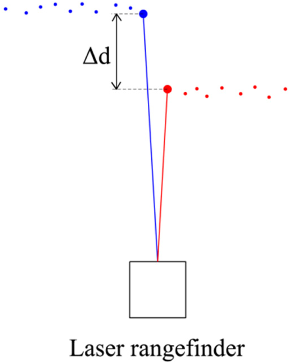
The principle of segmentation using threshold. Two segments are shown, the first one is marked by blue color and the second one is marked by red color. The distance between these segments is Δ.

Figure 2.

The example of segmentation using the threshold on real data points. Three segments are distinguishable by color.

In many cases, large segments, such as walls, are interrupted by small gaps. This produces the larger number of segments than there are real objects. A small gap is defined as one that does not consist of more than three data points. Therefore, such gap is not considered to be an object. Such case is shown in Figure 3, where small gap (black color) divides one large segment into two smaller segments. Hence, the algorithm was enhanced to account for such cases.

Figure 3.

The example of small gap, which divides one large segment (wall) into two smaller ones.

The enhancement of the algorithm involves the connection of two segments, which are separated by small gap. This connection can be done if two conditions are met.

The difference in measured distances of boundary points (points from the large segment, which are adjacent to the small gap) cannot exceed the threshold.

Both boundary points have to lie in specific surroundings (Figure 4).

Figure 4.

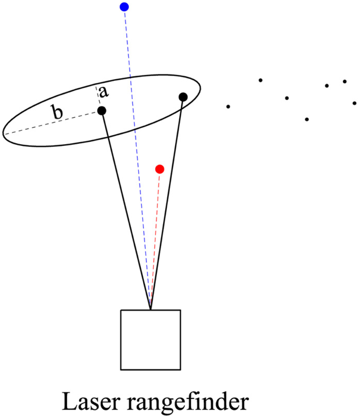
The second condition, which have to be fulfilled for the connection of two segments.

The data point lies in the surrounding area of a boundary point, when its coordinates (x_b , y_b ) are located inside of an ellipsis created around the boundary point (x_c , y_c ) and its semiaxes are equal to a = 1.5σ_y and b = 1.5σ_x . This means that it has to meet this condition

\frac{x_{b} - x_{c}}{a} + \frac{y_{b} - y_{c}}{b} < 1

The example of such enhanced segmentation can be seen in Figure 5. Such segmentation is computationally undemanding. However, if the gap is longer than three data points, the algorithm is unable to connect two segments belonging to the same object.

Figure 5.

The example of enhanced segmentation—segment one consists of two subsegments, which are divided by small gap.

From the previous examples, it is clear that some objects could be represented by smaller amounts of data. For example, a box in Figure 5 (green segment) is represented by 22 data points. The box consists of relatively flat surfaces and it can be represented by smaller amount of data. The basic idea of the proposed algorithm is to represent any shape by a set of line segments. The number and length of the line segments is directly dependent on the complexity of the measured shape and the required accuracy of representation. Given that the goal of the algorithm is to achieve the simplification of data, it is desirable that the object is represented by no more data than was necessary for its representation before the simplification. From the analytical geometry point of view, a line segment can be described by various forms. However, when working with objects, it is suitable to describe them by coordinates of end points. Hereby, line segments are expressed as a sequence of points, where the end point of one line segment is the starting point of the following line segment. Hence, a simplified object, which consists of n points, can be described at most by n-1 line segments. The principle of this algorithm is shown in Figure 6.

Figure 6.

The principle of algorithm used for simple representation of objects.

The angle between the data points was chosen as a measure of whether it is possible to exclude any data point

β_{i, j} = a cos (\frac{l_{j} - l_{i} cos (α_{j - i})}{\sqrt{l_{i}^{2} + l_{j}^{2} - 2 l_{i} l_{j} cos (α_{j - i})}})

where α_j-i is the angle between two consecutive measurements (Figure 7).

Figure 7.

The definition of angles used in data points exclusion.

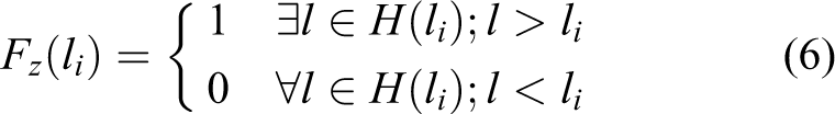
Measurements are corrupted by noise. This noise could cause that some data points fail to represent a real object precisely. Therefore, a threshold was proposed. Thus, the accuracy of object’s representation is affected by the threshold’s value. The condition which determines whether the data point will represent a new object is defined as follows

F_{v} (l_{i}) = (| β_{i - 1 - k, i} - β_{i, i + 1} |) < p

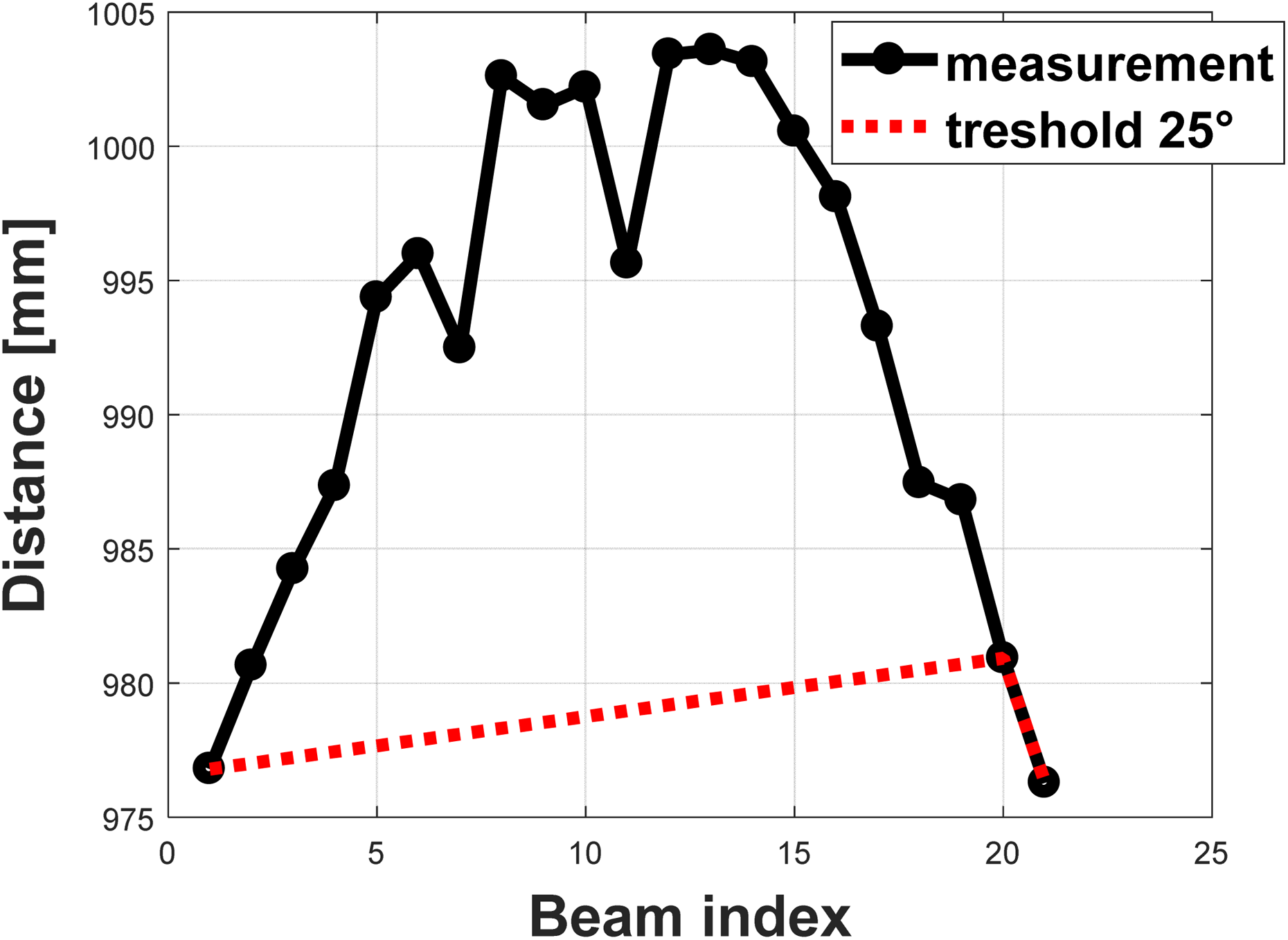
where p is the threshold, k is the index of last point, which is considered as object, β_i-1-k _,i is the angle pertaining to the data point l_i-1-k , and β_i _,i+1 is the angle pertaining to the data point l_i . If the condition is fulfilled, the data point is rejected from the representation of the object. Consequently, the value k is increased by 1 and next point l_i+1 is evaluated. If the condition is not fulfilled, the data point is considered as the boundary point of the line segment and the value k is set to 0. In this case, the data point is marked as the starting point of a line segment, and from this point, the condition is evaluated for the following data points. This algorithm was implemented along with the enhanced segmentation described earlier and the result of such segmentation is shown in Figure 8. In this case, the threshold p has the value 25°.

Figure 8.

The result of the algorithm, which applies the enhanced segmentation with threshold.

It is clear that the threshold affects both the accuracy of object’s representation as well as the number of skipped data points. The results for a simple object’s segmentation with various threshold values are shown in Figure 9.

Figure 9.

The segmentation of a simple object with various threshold values.

There are some shapes of objects, that is, objects with rounded edges, where the threshold between two data points is not exceeded; however, there is a significant change of angle. The proposed segmentation will not represent this object correctly (Figure 10). That is why two additional parameters were included. The first parameter describes the maximum number of data points that may be skipped in a row. The second parameter identifies the number of data points, from which the angle β_i,j is computed. While the first parameter improves the representation of the object’s shape, the second parameter increases the number of skipped points. As can be seen in Figure 11, the proposed algorithm now better represents the shape of the object in comparison with the results shown in Figure 10.

Figure 10.

The incorrect segmentation of object with rounded edges.

Figure 11.

Enhanced segmentation with threshold 25° and with the restriction of maximum skipped data points equal to 5.

The resulting algorithm has this form

F (l_{i}) = {\begin{matrix} 0 \land k = k + 1 & ((| {β^{'}}_{i - (1 + k) m, i} - {β^{'}}_{i, i + m} | < p) \lor (k < M)) \land (i mod m) \neq 0 \\ 1 \land k = 0 & ((| {β^{'}}_{i - (1 + k) m, i} - {β^{'}}_{i, i + m} | \geq p) \land (k \geq M)) \lor (i mod m) = 0 \end{matrix}

where M is the maximum number of skipped points, m is the number of data points, from which the angle β_i,j is computed, p is the threshold, and angle ${β^{'}}_{i, j}$ is computed as

{β^{'}}_{i, j} = \frac{1}{j - i} \sum_{h = 0}^{j - i - 1} β_{i + h, i + 1 + h}

F takes the zero value for a point that is skipped from an object’s representation and value 1 for a point that remains in the representation. The results for various settings of both parameters are shown in Figures 12 and 13.

Figure 12.

Enhanced segmentation with threshold 25° and for the varying number of maximum skipped data points for a simple object.

Figure 13.

Enhanced segmentation with threshold 25° and for the varying number of data points, from which the angle β_i _,j is calculated.

The proposed algorithm allows reduction of the number of points needed to represent objects. It also reduces the amount of memory and computing power needed. The degree of an object’s simplification can be set by various parameters. The first parameter is threshold, which determines the accuracy of the shape representation. The second parameter is the maximum number of skipped data points, which provides tracking of slowly changing shapes. The third parameter is the number of data points that serve in calculating the angle, which is used to evaluate whether the threshold was exceeded. With this parameter, it is possible to set the minimum amount of the object’s shape simplification. The disadvantage of this algorithm is the fact that the resulting simplification will be slightly different from the original shape with repeated measurements. It follows that it is not possible to compare two objects described by this algorithm. Therefore, another algorithm was proposed. This algorithm determines only those points that uniquely characterize objects. Such significant points are, for example, corners (Figure 14) or interruptions at the edges. These points represent extremes in measurements.

Figure 14.

Significant points in LRF measurement. LRF: laser range finder.

Since the LRF measurements are generated from one point, some objects are hidden by other objects and therefore some significant points are not recorded. Another consequence is the occurrence of apparent significant points—false extremes. These false extremes occur when the object in the foreground covers the object behind it. Consequently, the object in the background seems to be finished in the measurement (Figure 15). In reality, this is not true. False extremes are not stable in a time, because the object in the foreground may move or the LRF may move itself. This will also cause the movement of false extreme itself (Figure 16). Therefore, it is needed to distinguish whether it is apparent or real significant point.

Figure 15.

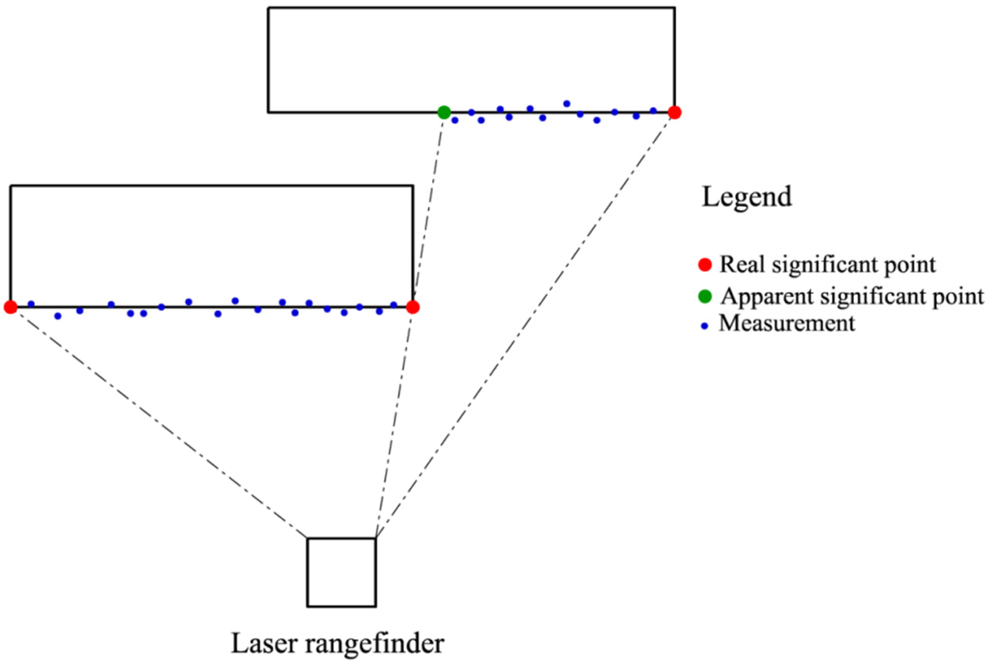
The occurrence of apparent significant points due to the covering of two objects.

Figure 16.

The movement of false extremes within the movement of LRF itself. LRF: laser range finder.

Proposed algorithm works with simplified objects, as it was mentioned earlier. The aim of the algorithm is to find real as well as apparent significant points. Each object is created at least from two significant points. Usually these points are outline points. Besides these outline points, each object may contain any number of significant points. Each apparent significant point must be also apparent outline point. Therefore, the first step of algorithm is the evaluation of outline points. If the outline point is real significant point, then the following function takes the value 1

F_{z} (l_{i}) = {\begin{matrix} 1 & \exists l \in H (l_{i}); l > l_{i} \\ 0 & \forall l \in H (l_{i}); l < l_{i} \end{matrix}

where the function H is the set of points l in the surroundings of the outline point l_i . Since there is always object from the one side for the outline point, the set is different for both outline points. Set for the first outline point contains these members

H (l_{i}) = [l_{i - 5}, l_{i - 4}, l_{i - 3}, l_{i - 2}, l_{i - 1}]

And for the second outline point contains these members

H (l_{i}) = [l_{i + 1}, l_{i + 2}, l_{i + 3}, l_{i + 4}, l_{i + 5}]

Outline point is considered as apparent significant point if its whole surrounding is closer to LRF and therefore it exists probably another real significant point, which is covered by nearer object. Another step of algorithm searches for significant points in inner parts of objects. Significant points in inner parts of objects are defined as real points, in which the object significantly changes its shape. Such changes are detected by the mutual position of line segments inside the objects. Following function is defined as

F_{t} (l_{i}, k) = {\begin{matrix} 0, k = 0 & ‖ l_{i} - l_{i - 1} ‖ < m L e n \\ 0, k = 0 & ‖ l_{i} - l_{i - 1} ‖ > m L e n \land ‖ l_{i} - l_{j} ‖ > m L e n \land γ_{i, j} \notin 〈 δ_{m}, δ_{M} 〉 \\ F_{t} (l_{i}, k = k + 1) & ‖ l_{i} - l_{i - 1} ‖ > m L e n \land ‖ l_{i} - l_{j} ‖ < m L e n \\ 1, k = 0 & ‖ l_{i} - l_{i - 1} ‖ > m L e n \land ‖ l_{i} - l_{j} ‖ > m L e n \land γ_{i, j} \in 〈 δ_{m}, δ_{M} 〉 \end{matrix}

where

\begin{array}{l} j = i + 1 + k \\ γ_{i, j} = 180 ° - (β_{i - 1, j} + α_{i}) + β_{i, j} \end{array}

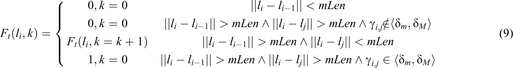
where mLen is minimal distance between points, δ_m and δ_M are lower and upper limit of angle γ, γ_i,j is angle between two line segments, and β_i,j is angle between points l_i and l_j , which is computed by equation. As it can be seen, algorithm compares angles between the line segments with the length greater than parameter mLen. In the case if the point l_i is too close to the previous point from simplified object, it will not be considered as significant point. If such point is not too close to the previous point from simplified object, and moreover the angle between the line segments is from the selected interval, this point will be evaluated as significant point. Special case may occur when the first point fulfills the distance condition, but the second point does not. In this case, the evaluation for the point l_i is repeated with the following point. The output of the algorithm applied on the simplified objects can be seen in Figure 17. Other experiments are shown in Figures 18 and 19.

Figure 17.

Significant points after applying of the proposed algorithm.

Figure 18.

Significant points after applying of the proposed algorithm (δ_m = 40° and δ_M = 140°).

Figure 19.

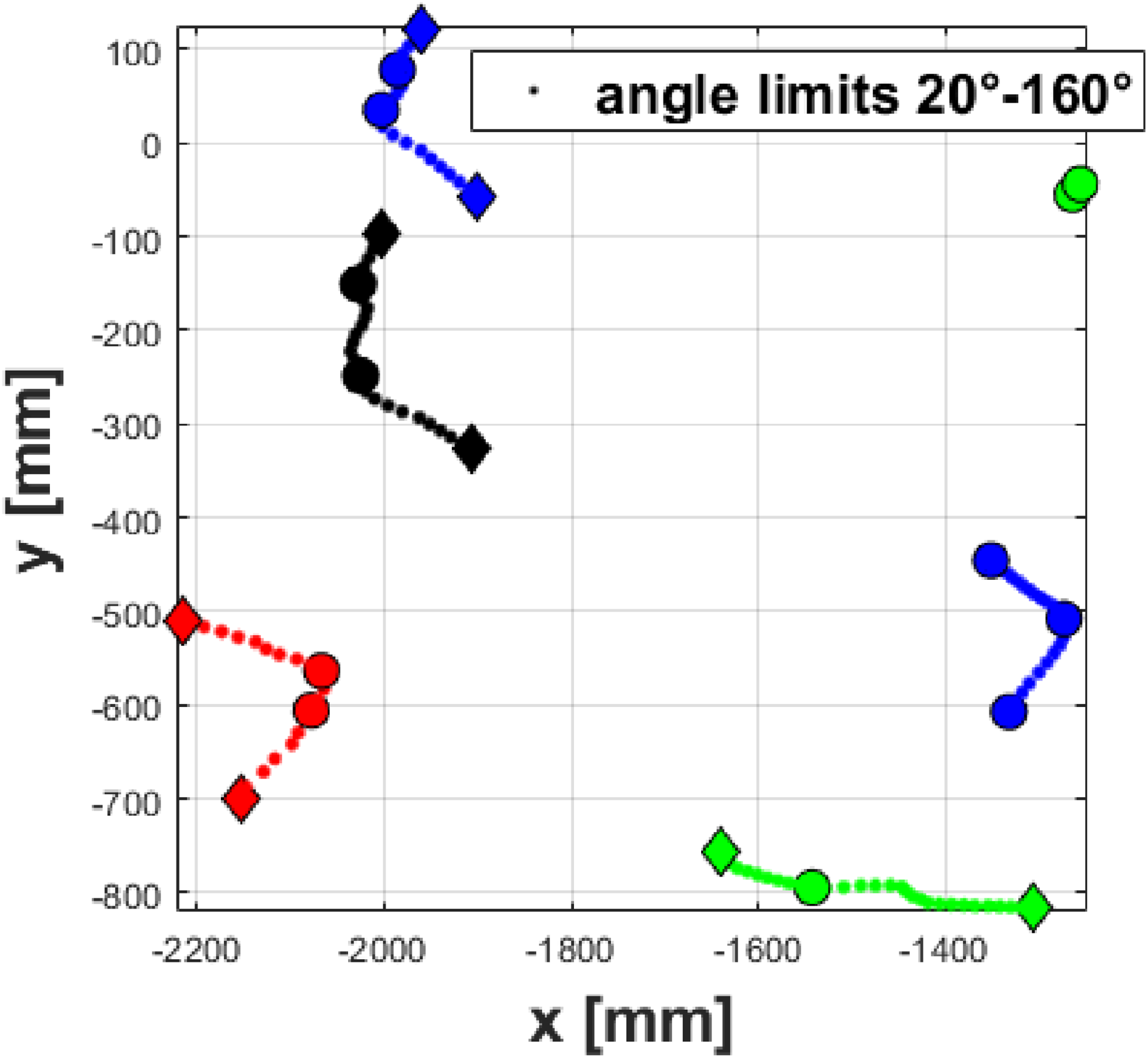
Significant points after applying of the proposed algorithm (δ_m = 20° and δ_M = 160°).

As it can be seen, proposed algorithm finds the significant points on the objects, which have meaning change in their shape. However, there may be objects, which do not contain such changes, but from the global point of view, the change is significant. Such objects have usually rounded shape. Therefore, another step in algorithm was proposed. This step is characterized as test of object’s eccentricity. If the object does not contain any inner significant point, the farthermost point from the object’s borders is the input to the test. If the distance of this point is greater than threshold, it is marked as significant point (Figure 20). The threshold is empirically stated and it is equal to 1/5 of distance between the border points of object.

Figure 20.

The significant points of rounded object after another enhancement of the proposed algorithm.

Proposed algorithm enables the description of objects by significant points. This algorithm is based on simplified object, whose principle was described above. The output of the algorithm may be modified by several thresholds, for example, minimal distance between object’s representation, minimal and maximal angle between the data points, or eccentricity of the object. The key aspect of the algorithm is distinguishing between real and apparent significant points. Such description of objects reduces memory demands without the loss of information.

Moving obstacles detection

Mobile robots are used in environments, which are dynamically changing and containing a lot of moving objects, for example, humans or other robots. Therefore, successful control (SLAM, navigation, etc.) of robot needs to take into consideration such objects. The proposed algorithm is based on the segmentation described in the previous section. Algorithm itself may be divided into three steps:

localization—formulated as a laser odometry based on the implementation of iterative closest point (ICP),⁵⁵

object matching—formulated as the correspondence searching of significant points based on kd-trees (Figure 21), and

moving obstacles detection.

Figure 21.

The correspondence searching of significant points based on kd-trees.

Moving obstacles detection is based on assumption that if the object moves, significant points of this object are moving too. Therefore, direction and distance of how far the object is moved are determined by the displacement of its significant points. The first step of the algorithm is looking for the correspondence between the significant points of particular objects in two consequent measurements. It is assumed that there is no notable change in the object’s shape, and the correspondence is determined by these steps as follows:

the construction of kd-tree from the significant points of the first measurement;

finding the two closest points in the second measurement for each significant point from the first measurement;

the arrangement of pairs of significant points by the shortest distance; and

the removal of pair, in which one significant point is contained in pair with shorter distance.

In the case that both significant points in pair are real, then the displacement of significant point in x- and y-axes is determined by the difference in coordinates

P [x, y] = P [v_{2}^{x} - v_{1}^{x}, v_{2}^{y} - v_{1}^{y}]

where v₁ and v₂ represent the significant points in pair and indexes x and y are the coordinates of these points. In the case that at least one point in the pair is apparent, the displacement is determined as a difference between apparent point and its perpendicular projection on the line. This connects the second significant point from the pair and adjacent significant point (Figure 22).

Figure 22.

The principle of displacement determination in the case of apparent significant point.

Then the displacement of significant point is defined as

P [x, y] = {\begin{matrix} P [v_{2}^{x} - o^{x}, v_{2}^{y} - o^{y}] & i f v_{2} is apparent significant point \\ P [o^{x} - v_{1}^{x}, o^{y} - v_{1}^{y}] & i f v_{1} is apparent significant point \end{matrix}

where o represents the point situated on the line, which connects the second significant point from the pair and adjacent significant point. If v ₁ is apparent significant point, then the coordinates of o are defined as

\begin{array}{l} o_{x} = v_{1}^{x} + (v_{2}^{y} - v_{p}^{y}) s \\ o_{y} = v_{1}^{y} + (v_{p}^{x} - v_{2}^{y}) s \end{array}

where v_p is adjacent significant point and s is defined as

s = \frac{v_{2}^{x} - v_{1}^{x} + (v_{p}^{x} - v_{2}^{y}) . \frac{(v_{2}^{y} - v_{p}^{y}) (v_{1}^{y} - v_{2}^{y}) + (v_{p}^{x} - v_{2}^{y}) (v_{2}^{x} - v_{1}^{x})}{(v_{p}^{y} - v_{2}^{y}) (v_{2}^{y} - v_{p}^{y}) - {(v_{p}^{x} - v_{2}^{y})}^{2}}}{(v_{2}^{y} - v_{p}^{y})}

Resultant displacement of the object is calculated as the average from every displacement of each significant point of the object

T [x, y] = \frac{1}{n} \sum_{i = 1}^{n} P_{i} [x, y]

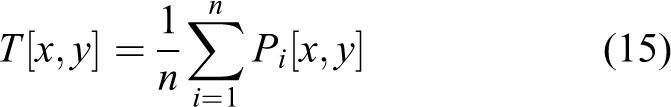
where n is the number of significant points.

For the needs of mobile robots, it is needed to detect moving obstacles approximately with the same speed as the speed of the robot. Used robot is capable to achieve the speed up to 1 m/s. Commonly used LRFs are working with frequencies up to several dozen hertz. When the speed of the robot reaches 1 m/s, the difference between two consequent measurements may reach 50 mm. However, this difference can appear in the measurements of static objects. Therefore, it is not possible to distinguish if the object is static or it is moving. From this reason, the detection of moving obstacle is based on several consequent measurements. In the case of static obstacle, the displacement should be rated with zero mean variance of measurement. In the case of moving obstacle, this value should increase in time. The condition, moving obstacle is identified, is defined as

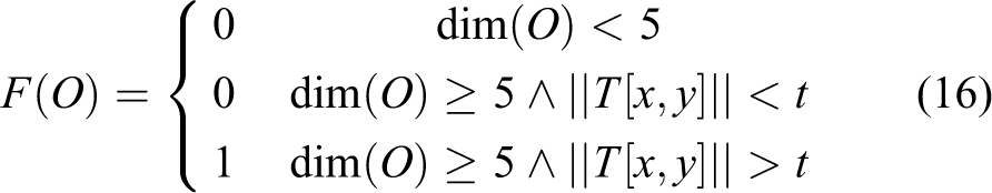
F (O) = {\begin{matrix} 0 & dim (O) < 5 \\ 0 & dim (O) \geq 5 \land ‖ T [x, y] ‖ < t \\ 1 & dim (O) \geq 5 \land ‖ T [x, y] ‖ > t \end{matrix}

where dim represents the dimension of object O, that is, how many times it was measured. The value $‖ T [x, y] ‖$ defines the overall displacement of the object and t represents threshold. If it is exceeded, the object is considered as moving. This threshold was determined experimentally and it is equal to 200 mm. As the resultant displacement of the object is calculated as the average from every displacement, one wrong calculation of displacement may impair the overall displacement. Therefore, the maximal consequent measurements taken into account were defined. This value was equal to 10.

Verification and experiments

Simulated environment with several types of objects (e.g. circular object) was chosen to verify proposed segmentation. LRF was placed into the origin of coordinate system. Selected parameters of the algorithm are shown in Table 1. These parameters are derived on the basis of LRF’s probabilistic model. Particular model of Hokuyo UTM-30LX was defined by Dekan et al.⁵³ All the parameters mentioned in Table 1 are determined on the basis of LRF’s resolution and accuracy. And they are not dependent on the type of environment, which was proven by Dekan et al.⁵³

Table 1.

Parameters of proposed algorithm.

Object’s simplification	Value of parameter
Threshold p	25°
Minimal skipped data points	1
Maximal skipped data points	5
Significant points of objects
δ_m	40°
δ_M	140°

As it was expected (Figure 23), simulated environment was divided into several objects. Mentioned object’s boundary points represent apparent significant points. As it can be also seen, the points of simplified segments are tracing significant points. However, for better evaluation of such tracing, some numerical formulations have to be mentioned. For this purpose, root mean square error was chosen as

RMSE = \sqrt{\frac{\sum_{i = k}^{m} {(\frac{cos (l_{i}^{α}) . l_{i} . a + sin (l_{i}^{α}) . l_{i} . b + c}{\sqrt{a^{2} + b^{2}}})}^{2}}{m - k}}

where k and m represent indexes of two consequent significant points from the simplified object and l_i stands for ideal measurement in polar coordinates. Parameters a, b, and c represent parameters of the line obtained from significant points of simplified object k and m

\begin{array}{l} a = - \frac{sin (l_{m}^{α}) . l_{m} - sin (l_{k}^{α}) . l_{k}}{cos (l_{m}^{α}) . l_{m} - cos (l_{k}^{α}) . l_{k}} \\ b = 1 \\ c = - \frac{sin (l_{k}^{α}) . l_{k} - (sin (l_{m}^{α}) . l_{m} - sin (l_{k}^{α}) . l_{k}) . cos (l_{k}^{α}) . l_{k}}{cos (l_{m}^{α}) . l_{m} - cos (l_{k}^{α}) . l_{k}} \end{array}

Figure 23.

The principle of displacement determination in the case of apparent significant point.

Results are shown in Table 2. As it can be seen, RMSE for simplified objects is comparable with RMSE for filtered measurements. Significant worse results emerged within circular object (Figure 24). Despite this, the level of data degradation is negligible for the needs of mobile robotics. The compression rate is 1:45 and therefore the data degradation for such type of objects is acceptable. In this case, the number of recorded points was reduced from 1080 points to 24 points.

Table 2.

RMSE for measurement with noise, filtered measurement, and simplified objects.

Object number	RMSE noise (mm)	RMSE filtered (mm)	RMSE simplified (mm)
1	8.7854	5.1281	0.8164
2	7.2041	4.2920	2.9088
3	6.7285	3.9081	8.6145
4	9.1140	5.2429	3.2143
5	8.4811	3.9524	3.9433
6	8.5842	4.4363	1.8828
7	7.2627	4.3350	3.9111
8	7.0128	4.1360	5.6573
9	7.8536	4.4771	15.5939
10	6.2734	3.5564	4.2818

RMSE: root mean square error.

Figure 24.

The measurement of circular object and corresponding simplification of such object.

Proposed algorithms enable significant simplification of data based on sensed environment. This simplification does not cause loss of information, such as corners of objects and so on. Proposed segmentation can also be used in cases where the high accuracy is required (SLAM, detection of moving obstacles, etc.).

Proposed detection of moving obstacles depends on the segmentation of data points, the detection of significant points, and the localization of mobile robot. The localization of mobile robot was proposed in the form of laser odometry with ICP implemented.⁵⁵ The accuracy of segmentation and the detection of significant points depend on the quality of data preprocessing. Therefore, it can be stated that the accuracy of object’s correspondence between two consequent laser scans is depending on proposed algorithms. However, numeric expression of this accuracy is not possible to evaluate, because correspondence between the individual measurements vary in time. This is because the objects may be segmented in different ways due to the robot’s motion. However, even if the object is segmented inappropriately, this can be later corrected and for example two wrong segmented objects may be correctly connected into the single one. This inaccuracy is proportional to the complexity of mapped environment. If the environment contains several bigger homogenous objects, the overall accuracy of proposed algorithms will be better than in the case with small and densely placed objects (e.g. chair legs). Moreover, the overall accuracy will be significantly changing under the influence of moving obstacles and the motion of robot itself. Namely, these motions will cause the change of objects’ shape, because the mutual overlay of objects will change. Following four tests were made to demonstrate these claims:

static robot and static environment,

moving robot and static environment,

static robot and single moving obstacle, and

moving robot and single moving obstacle.

All the tests were performed in laboratory with tables, chairs, paper boxes, and other nonhomogenous objects. Such environment is quite challenging and variable for data processing. Moreover, LRF was not fixed, whereby the systematic errors of odometry were simulated.

The result of the first test (static robot and static environment) is shown in Figure 25. As it can be seen, despite the robot does not change its position, the number of objects vary in time. This is caused by noise, which causes different segmentation and identification of significant points. Consequently, correspondence between two consequent measurements contains some wrong paired objects. It can be also seen that the laser odometry partially suppresses these small variations, but it will also generate incorrect change in the robot’s position.

Figure 25.

The number of identified objects (segments) in environment using odometry and laser odometry as localization method (static robot and static environment).

The result of the second test (moving robot and static environment) is shown in Figure 26. As it can be seen, there is a significant difference in the number of objects between usage of odometry and laser odometry. This was caused by not fixed position of LRF. Consequently, small shift of objects between measurements caused wrong objects’ pairing. The number of objects was gently increased compared to the previous test. This was caused by the change in the position of apparent significant points introduced by the motion of the robot.

Figure 26.

The number of identified objects (segments) in the environment using odometry and laser odometry as localization method (moving robot and static environment).

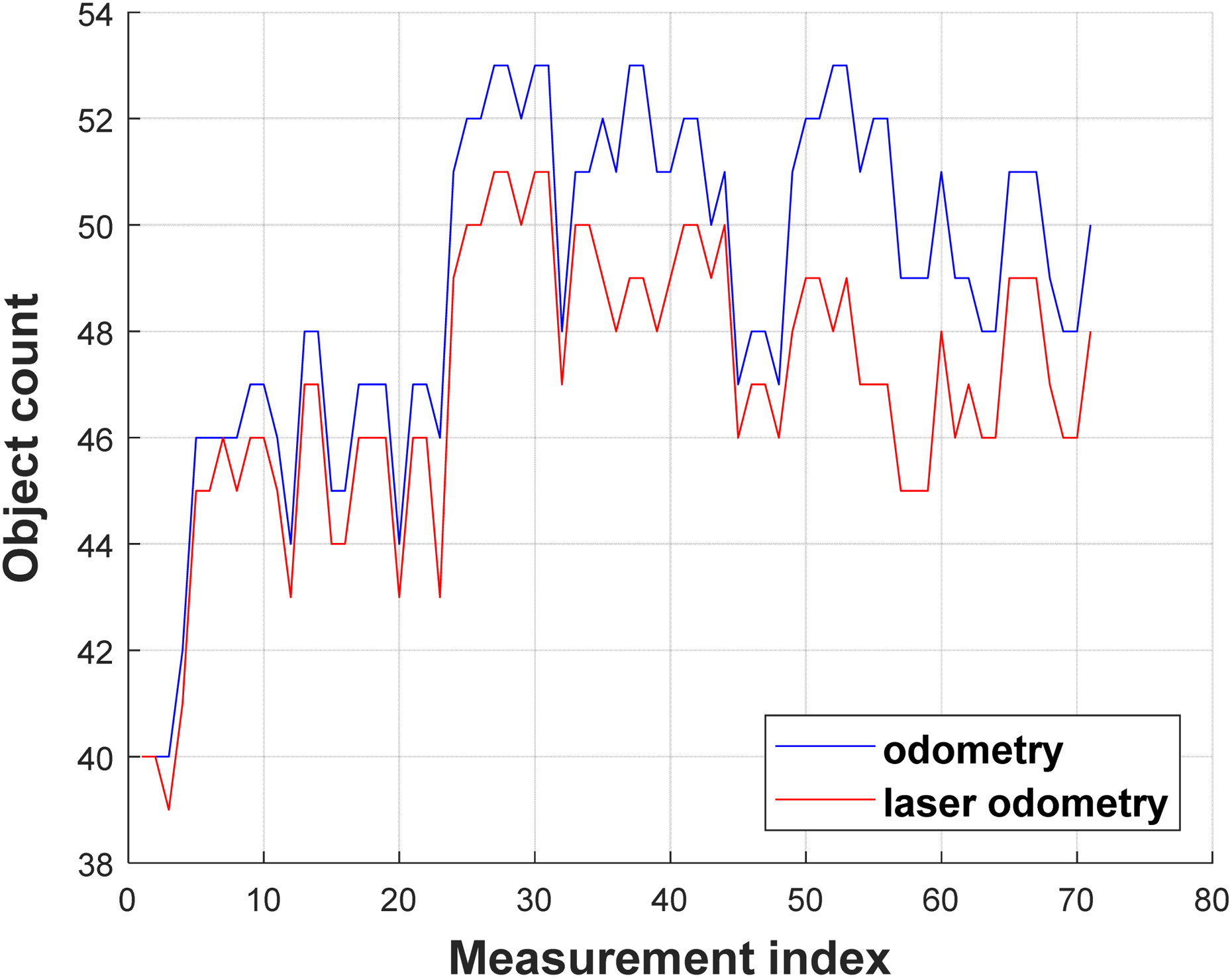
The tests with moving obstacles (Figure 27) showed growth in the number of objects in time. In the case of static robot, the growth compared to the first test is minimal, because moving obstacle affected only objects in its near surrounding. On the contrary, the motion of the robot is affecting the objects in the whole measuring range. However, it must be said that many of these incorrectly identified objects disappeared over several measurements and the number of steady detected objects was the same for each test.

Figure 27.

The number of identified objects (segments) in the environment using odometry and laser odometry as localization method (single moving obstacle).

The important aspect of proposed algorithms is ability to determine the object’s motion.

Figures 28 and 29 show the movement of objects between individual measurements in the case with moving obstacle. Significant difference can be seen in overall movements of objects (Figures 30 and 31), where single object significantly exceeds the limit, which can be considered as a noise.

Figure 28.

Calculated movement of objects in the direction of x-axis with single moving obstacle.

Figure 29.

Calculated movement of objects in the direction of y-axis with single moving obstacle.

Figure 30.

Calculated overall movement of objects in the direction of x-axis with single moving obstacle.

Figure 31.

Calculated overall movement of objects in the direction of y-axis with single moving obstacle.

The next step is to determine which object is moving. Number of moving objects in the static environment is shown in Figure 32, and the same parameter in environment with single moving obstacle is shown in Figure 33. As it can be seen, in all the tests, except one, at least one object was evaluated as moving. In the case of environment with single moving obstacle, at least one moving obstacle was identified approximately in the same time, and it retained moving until the end of the test. Remaining incorrectly identified moving obstacles remained evaluated as moving only for a short time. It can be stated that the proposed algorithms worked very well for this type of environment. Worse results were obtained within the tests with no moving obstacles. The worst results were achieved in the case of moving robot, whose position was determined from odometry. This error was caused by loosely attached LRF, which caused apparent movement of objects in the environment. However, before the method will be declared as nonfunctional, it should be recognized what types of objects are identified as incorrect (Figure 34, objects 21 and 49 highlighted in green). More or less, there are objects in the background with very unstable shape and they are influenced by many factors such as the occasional capture of the legs of chairs and reflections from shiny surfaces in the area. This incorrectly identified object does not create any constant movement, but it creates only oscillations around the mean value of its true position.

Figure 32.

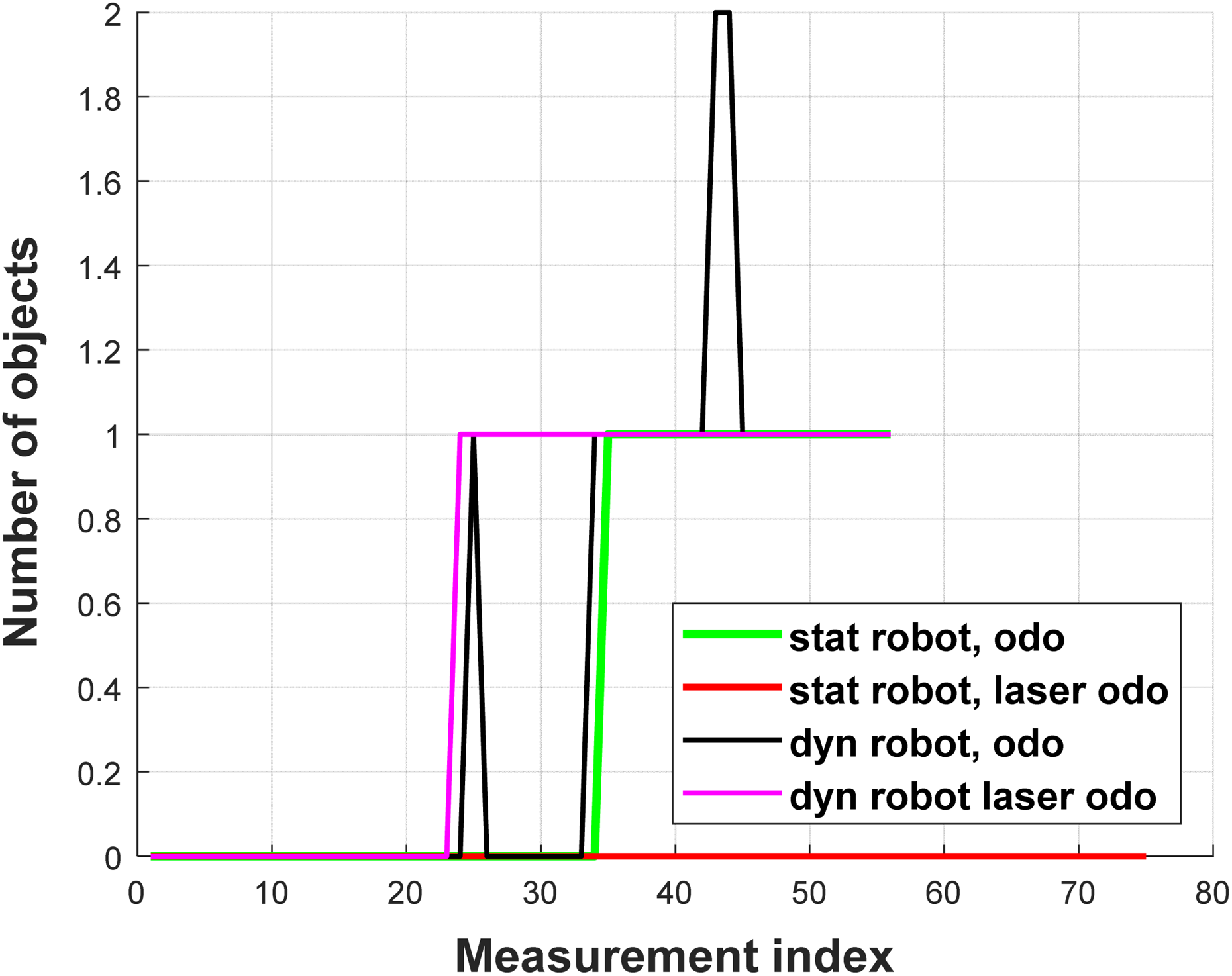
The number of objects identified as moving obstacles in the static environment.

Figure 33.

The number of objects identified as moving obstacles in the environment with single moving obstacle.

Figure 34.

The part of experiment on the real robot.

Conclusion

In the article, multiple algorithms for LRF data processing were proposed. First algorithm was segmentation, which considers small interruption in measured objects and thus suppresses over-segmentation. Simplification algorithm was then used on these segments. The advantage of this proposed algorithm is that it does not change the data structure of the measured space, yet it greatly reduces the amount of points needed for its representation. The precision of the algorithm can be adjusted per the needs of the application. Significant points were chosen from the simplified segments, and algorithm for distinction of apparent and real significant points was proposed. The significant points were used as object description for moving obstacle detection. Proposed detection of moving obstacles based on the LRF measurements was verified by the complex set of tests. Algorithm reliably identifies the moving objects. However, provided tests show that if the environment contains obstacles, with the shape at the limit of LRF resolution, some static objects may be identified as moving. Such incorrect identification can be suppressed by the additional processing of calculated movements. Generally, the proposed algorithm can be used in any type of robot and with cheap LRF already available in the market. Another advantage of proposed algorithm is simple implementation and overall low computational complexity. This algorithm makes it easy to use even in cheaper robots that have a wider application, for example, in households, such as those found in laboratories. In the future work, we intend to use proposed moving obstacle detection algorithm as part of the Vector Field Histogram with Time Dependent Tree (VFH*TDT) proposed by Babinec et al.⁵⁶ Moving obstacle detection algorithm will be implemented as a support algorithm for SLAM solutions in environment with dynamic objects. SLAM algorithms should benefit from moving obstacles refusal during the map creation especially in the case where the amount of such objects is significant and standard SLAM fails.

Footnotes

Declaration of conflicting interests

The author declared no potential conflicts of interest with respect to the research, authorship, and/or publication of this article.

Funding

The author disclosed receipt of the following financial support for the research, authorship, and/or publication of this article: This work was supported by Agentúra na Podporu Výskumu a Vývoja, APVV-16-0006; ITMS, ITMS 26240220033; and Vedecká Grantová Agentúra MŠVVaŠ SR a SAV, 1/0752/17.

References

Kelemen

Virgala

Kelemenová

. Distance measurement via using of ultrasonic sensor. J Autom Control 2015; 3(3): 71–74.

Konolige

Augenbraun

Donaldson

. A low-cost laser distance sensor. In: 2008 IEEE international conference on robotics and automation, Pasadena, CA, May 2008, pp. 3002–3008. IEEE. DOI: 10.1109/ROBOT.2008.4543666.

Qian

Fang

. Mobile robot self-localization in unstructured environments based on observation localizability estimation with low-cost laser range-finder and RGB-D sensors. Int J Adv Robot Syst 2016; 13: 1729881416670902.

Surmann

Lingemann

Nüchter

. A 3D laser range finder for autonomous mobile robots. In: Proceedings of the 32nd international symposium on robotics (ISR’01), Seoul, Korea, April 2001, pp. 153–158.

Nejad

Olyaee

. Comparison of TOF, FMCW and phase-shift laser range-finding methods by simulation and measurement. Quart J Technol Educ 2006; 1: 11–18.

Smith

. Active sensors for local planning in mobile robotics, Vol. 26. World Scientific, 2001; pp. 177–184.

Bazin

Journet

. A new laser range-finder based on FMCW-like method. In: Quality measurement: The indispensable bridge between theory and reality (No Measurements? No science! Joint conference - 1996: IEEE instrumentation and measurement technology conference and IMEKO Tec, Brussels, Vol. 1, 1996, pp. 90–93. DOI: 10.1109/IMTC.1996.507354.

Dietmayer

Sparbert

Streller

. Model based object classification and object tracking in traffic scenes from range images. In: Proceedings of IV IEEE intelligent vehicles symposium, Vol. 200, May 2001.

RPLIDAR 360° Laser Scanner. https://www.slamtec.com/en/Lidar/A1 (accessed 12 December 2017).

10.

Pomerleau

Breitenmoser

Liu

. Noise characterization of depth sensors for surface inspections. In: 2012 2nd international conference on applied robotics for the power industry, September 2012, pp. 16–21. IEEE.

11.

Singh

Sharma

Kumar

. Mathematical approach for the removal of specular reflection of laser rangefinder. Int J 2001; 2: 186–188.

12.

Herbert

Krotkov

. 3D measurements from imaging laser radars: how good are they? Journal Image and Vision Computing 1992; 10(3): 170–178. DOI: 10.1016/0262-8856(92)90068-E.

13.

Castellanos

Martinez

Neira

. Simultaneous map building and localization for mobile robots: a multisensor fusion approach. In: Proceedings. 1998 IEEE international conference on robotics and automation, Vol. 2, May 1998, pp. 1244–1249. IEEE.

14.

Mader

Westfeld

Maas

. An integrated flexible self-calibration approach for 2D laser scanning range finders applied to the Hokuyo UTM-30LX-EW. Int Arch Photogram Remote Sens Spat Inform Sci 2014; 40(5): 385.

15.

Cook

. Mobile robots: navigation, control and remote sensing. Hoboken, NJ: John Wiley & Sons, 2011.

16.

Thrun

. Probabilistic robotics. Communic ACM 2002; 45(3): 52–57. DOI: 10.1145/504729.504754.

17.

. Mixed pixels removal of a laser rangefinder for mobile robot 3-D terrain mapping. In: 2008 International conference on information and automation, Changsha, June 2008, pp. 1153–1158. IEEE. DOI: 10.1109/ICINFA.2008.4608173.

18.

Vandapel

Huber

Kapuria

. Natural terrain classification using 3-D ladar data. In: Proceedings ICRA’04. 2004 IEEE international conference on robotics and automation, Vol. 5, April 2004, pp. 5117–5122. IEEE.

19.

Premebida

Nunes

. Segmentation and geometric primitives extraction from 2D laser range data for mobile robot applications. Robotica 2005; 2005: 17–25.

20.

Zalud

Kocmanova

Burian

. Calibration and evaluation of parameters in a 3D proximity rotating scanner. Elekt Elektrotech 2015; 21(1): 3–12. DOI: 10.5755/j01.eee.21.1.7299.

21.

Einsele

. Real-time self-localization in unknown indoor environment using a panorama laser range finder. In: IROS’97, Proceedings of the 1997 IEEE/RSJ international conference on intelligent robots and systems, Grenoble, Vol. 2, September1997, pp. 697–702. IEEE. DOI: 10.1109/IROS.1997.655087.

22.

Santos

Faria

Soares

. Tracking of multi-obstacles with laser range data for autonomous vehicles. In: Proceeding 3rd National festival of robotics scientific meeting, May 2003, pp. 59–65.

23.

Borges

Aldon

. Line extraction in 2d range images for mobile robotics. J Int Robot Syst 2004; 40(3): 267–297. DOI: 10.1023/B:JINT.0000038945.55712.65.

24.

Borges

Aldon

. A split-and-merge segmentation algorithm for line extraction in 2D range images. In: Proceedings 15th international conference on pattern recognition. ICPR-2000, Barcelona, Vol. 1, 2000, pp. 441–444. DOI: 10.1109/ICPR.2000.905371.

25.

Siadat

Kaske

Klausmann

. An optimized segmentation method for a 2D laser-scanner applied to mobile robot navigation. In: Proceedings of the 3rd IFAC symposium on intelligent components and instruments for control applications, June 1997, pp. 153–158.

26.

Nguyen

Martinelli

Tomatis

. A comparison of line extraction algorithms using 2D laser rangefinder for indoor mobile robotics. In: 2005 IEEE/RSJ international conference on intelligent robots and systems, August 2005, pp. 1929–1934. DOI: 10.1109/IROS.2005.1545234.

27.

Zhang

Ghosh

. Line segment based map building and localization using 2D laser rangefinder. In: proceedings 2000 ICRA. Millennium conference. IEEE international conference on robotics and automation. Symposia proceedings (Cat. No.00CH37065), San Francisco, CA, Vol. 3, 2000, pp. 2538–2543. DOI: 10.1109/ROBOT.2000.846410.

28.

Norouzi

Yaghobi

Siboni

. Recursive line extraction algorithm from 2d laser scanner applied to navigation a mobile robot. In: 2008 IEEE international conference on robotics and biomimetics, Bangkok, February 2009, pp. 2127–2132. DOI: 10.1109/ROBIO.2009.4913331.

29.

Yunlong

Heming

Qingchen

. Research on robot SLAM based on linear feature environment. Adv Inform Sci Ser Sci 2013; 5(3): 252.

30.

Garulli

Giannitrapani

Rossi

. Mobile robot SLAM for line-based environment representation. In: Proceedings of the 44th IEEE conference on decision and control, December 2005, pp. 2041–2046. IEEE. DOI: 10.1109/CDC.2005.15824611.

31.

Rueda

Udupa

Bai

. Local curvature scale: a new concept of shape description. In: Proc. SPIE 6914, medical imaging 2008: Image processing, 69144Q, 11 March 2008, pp. 69144Q–69144Q. International Society for Optics and Photonics. DOI: 10.1117/12.770444.

32.

Krejsa

Vechet

. Searching for features in laser rangefinder scan via combination of local curvature scale and human obstacles detection. In: Mechatronics, 2013, pp. 599–606. Cham: Springer International Publishing.

33.

Nunez

Vazquez-Martin

del Toro

. Feature extraction from laser scan data based on curvature estimation for mobile robotics. In: Proceedings 2006 IEEE international conference on robotics and automation, 2006. ICRA 2006, Orlando, FL, May 2006, pp. 1167–1172. IEEE. DOI: 10.1109/ROBOT.2006.1641867.

34.

Kocmanova

Zalud

Chromy

. 3D proximity laser scanner calibration. In: 2013 18th International conference on methods & models in automation & robotics (MMAR), Miedzyzdroje, August 2013, pp. 742–747. DOI: 10.1109/MMAR.2013.6670005.

35.

Lingemann

Nüchter

Hertzberg

. High-speed laser localization for mobile robots. Robot Auton Syst 2005; 51(4): 275–296.

36.

Prassler

Scholz

Elfes

. Tracking multiple moving objects for real-time robot navigation. Auton Robot 2000; 8(2): 105–116.

37.

García-Pérez

García-Alegre

Ribeiro

. Perception and tracking of dynamic objects for optimization of avoidance strategies in autonomous piloting of vehicles. In: Spatial cognition IV. Reasoning, action, interaction: International conference spatial cognition, Frauenchiemsee, Germany, 11–13 October 2004, pp. 500–517. Berlin, Heidelberg: Springer. DOI: 10.1007/978-3-540-32255-9_27.

38.

Wolf

Sukhatme

. Mobile robot simultaneous localization and mapping in dynamic environments. Auton Robot 2005; 19(1): 53–65.

39.

Himstedt

Maehle

. Online semantic mapping of logistic environments using RGB-D cameras. Int J Adv Robot Syst 2017; 14(4): 1729881417720781.

40.

Kluge

Köhler

Prassler

. Fast and robust tracking of multiple moving objects with a laser range finder. In: Proceedings 2001 ICRA. IEEE international conference on robotics and automation (Cat. No.01CH37164), Vol. 2, May 2001, pp. 1683–1688. IEEE. DOI: 10.1109/ROBOT.2001.932853.

41.

MacLachlan

Mertz

. Tracking of moving objects from a moving vehicle using a scanning laser rangefinder. In: 2006 IEEE intelligent transportation systems conference, Toronto, Ont., September 2006, pp. 301–306. IEEE. DOI: 10.1109/ITSC.2006.1706758.

42.

Mendes

Bento

Nunes

. Multi-target detection and tracking with a laser scanner. In: IEEE intelligent vehicles symposium, June 2004, pp. 796–801. IEEE. DOI: 10.1109/IVS.2004.1336486.

43.

Rebai

Benabderrahmane

Azouaoui

. (2009). Moving obstacles detection and tracking with laser range finder. In: ICAR 2009. international conference on advanced robotics, June 2009, pp. 1–6. IEEE.

44.

Sukop

Varga

Jánoš

. Very simple optical sensor to direct and recognition objects for mobile robots. In: Ukraine - EU. Modern technology, business and law - chernihiv: chernihiv national university of technology, 19–23 April 2016, pp. 330–331.

45.

Wang

Thorpe

. Simultaneous localization and mapping with detection and tracking of moving objects. In: Proceedings 2002 IEEE international conference on robotics and automation (Cat. No.02CH37292), Washington, DC, 2002, pp. 2918–2924. IEEE. DOI: 10.1109/ROBOT.2002.1013675.

46.

Becker

Hall

Jensen

. The use of obstacle motion tracking for car-like mobile robots collision avoidance in dynamic urban environments. In: Proceeding of XII international symposium on dynamic problems of mechanics–DINAME, February 2007.

47.

Montesano

Minguez

Montano

. Modeling the Static and the Dynamic Parts of the Environment to Improve Sensor-based Navigation. In: Proceedings of the 2005 IEEE international conference on robotics and automation, April 2005, pp. 4556–4562. IEEE. DOI: 10.1109/ROBOT.2005.1570822.

48.

Schulz

Burgard

Fox

. Tracking multiple moving targets with a mobile robot using particle filters and statistical data association. In: Proceedings 2001 ICRA. IEEE international conference on robotics and automation (Cat. No.01CH37164), Vol. 2, 2001, pp. 1665–1670. IEEE. DOI: 10.1109/ROBOT.2001.932850.

49.

Wang

Thorpe

Thrun

. Simultaneous localization, mapping and moving object tracking. Int J Robot Res 2007; 26(9): 889–916.

50.

Lyons

DM.

Cluster computing for robotics and computer vision. Hackensack, NJ: World Scientific Publishing Co. Pte. Ltd., 2011.

51.

Krishna

Kalra

. Detection, tracking and avoidance of multiple dynamic objects. J Int Robot Syst 2002; 33(4): 371–408.

52.

Monteiro

Premebida

Peixoto

. Tracking and classification of dynamic obstacles using laser range finder and vision. In: Proceeding of the IEEE/RSJ international conference on intelligent robots and systems (IROS), 2006, pp. 1–7.

53.

Dekan

Duchoň

Babinec

. Versatile approach to probabilistic modeling of Hokuyo UTM-30LX. IEEE Sens J 2016; 16(6): 1814–1828.

54.

Hargaš

Hrianka

Koniar

. Image processing and analysis: a practical approach – text book. Žilina: University of Žilina, 2008.

55.

Martínez

González

Morales

. Mobile robot motion estimation by 2D scan matching with genetic and iterative closest point algorithms. J Field Robot 2006; 23(1): 21–34.

56.