Sage Journals: Discover world-class research

Abstract

Monitoring the field of operation of an underwater vehicle is crucial during missions near the sea floor. The forward-looking sonar is often the only available sensor for the observation of the ambient turbid water environment. Sonar image registration is not only a first step towards a panoramic mosaic but it also provides an initial motion parameter estimation for the vehicle self-localization and navigation. In this article, a peripheral mutual information (PMI) maximization method is proposed for the sonar image registration. Peripheral mutual information is inspired by regional mutual information (RMI) which makes use of the closed-form solution for the Shannon entropy by the assumption that the data vectors made of neighbouring pixels are normally distributed, an assumption that ignores correlations between the pixels in sonar images. To accommodate the fact that the neighbouring pixels show dependencies due to acoustic reverberation and dispersion, only the peripheral information in the neighbourhood of a pixel is used in peripheral mutual information for the calculation of the mutual information. Experiments show that the peripheral mutual information registration function is much smoother than that of regional mutual information. Further experiments on the two-dimensional forward-looking sonar image registration demonstrate the efficiency of peripheral mutual information.

Keywords

Forward-looking sonar image registration regional mutual information peripheral mutual information

Introduction

The forward-looking sonar is an important monitoring device for the sea floor environments. For example, as more and more pipelines are laid on the seabed to facilitate the exploration and exploitation of marine resources, there is an increasing demand to deploy autonomous underwater robots to perform pipeline construction and maintenance. In order to detect pipelines that are spanned over the seabed, or buried or half-buried under the seabed, various sensors are required, such as cameras, side-scan sonars, multibeam sonars, sub-bottom profilers and magnetometers. The sensor data are analysed either by an on-board operator¹ or automatically within the underwater vehicle.² Although post-action inspections are necessary to identify potential risks, predictive measures should also be taken to enhance the safety of the pipelines, that is, monitoring the pipeline laying process.

Unfortunately, when a pipeline laying robot operates on the seabed, mud and sand can be stirred up easily, leading to turbid waters, which decreases the visual distance of optic sensors drastically. In this case, the forward-looking sonar is essentially the only available sensor that can be used to observe the immediate environment. On the one hand, the emergence of the high-frequency forward-looking sonar (e.g. BlueView [Teledyne BlueView, Inc., Seattle, Washington] and DIDSON [soundmetrics, Bellevue, Washington]) enables the underwater robots to achieve precise observations in turbid waters.³ On the other hand, only a very limited area can be scanned in each frame because of the restricted coverage of the acoustic device.⁴ Therefore, local sonar images should be stitched to form a panoramic map that supports the analysis of macroscopical geographic and geomorphic conditions. This will also be useful for the registration of forward-looking sonar images in a wide range of applications, such as active hydrothermal vent observation⁵ and wreck salvage.⁶

The image stitching process can generally be decomposed into two steps, image-pair registration and global error reduction.^7,8 An appropriate image registration method does not only provide cues for the global feature mapping but also alleviates the post-adjustment costs. Moreover, compared to the sonar image registration, global adjustment does not depend on the prior knowledge of the underwater acoustic imaging mechanism. Therefore, only image-pair registration is considered in this article.

Consider two images f( x ) and g( x ) that were taken by the forward-looking sonar at different times. If the images are overlapping, that is, if a transformation

x_{2} = T x_{1}

can be found that relates pixel x ₁ in image f with pixel x ₁ in image g, then we should expect a transformation matrix that minimizes the matching error within the overlapping area

T^{*} = arg min \sum_{(x_{1}, x_{2})} | f (x_{1}) - g (x_{2}) |

In image registration, we aim at optimizing the transformation matrix T which is determined by the vector of motion parameter Θ, which typically includes translation (Δx, Δy), elevation Δz, rotation θ, tilt ϕ and roll ψ. Three types of methods have been proposed for forward-looking sonar image registration.

The first type is based on feature point extraction and is directly derived from its counterparts in optic image processing. In the preprocessing stage, interest feature points are extracted from each image and a matching strategy is used to construct the feature point pairs $(x_{1}^{i}, x_{2}^{j})$ , where the superscripts i and j refer to the ith and jth feature point in f and g, respectively. Then, a group of equations in the form of equation (1) can be built and the motion parameters can be estimated by the least square method. In 2005, Negahdaripour and Sabzmeydani⁹ extracted Harris corner points from forward-looking sonar images and proposed a windowed-searching skill to perform the pairwise matching. Kim et al.¹⁰ also proposed a similar scheme, with the only difference that the Harris corner points are extracted from the third and the fourth layers in the Gaussian pyramid. However, the feature points extracted by the two methods tend to contain too much noise, thus compromising the matching process. In 2011, Negahdaripour et al.¹¹ pointed out that it is difficult to extract scale-invariant feature transform (SIFT) feature points from forward-looking sonar images of a natural, unstructured seabed.

The second category belongs to cluster- or region-based methods. Though each single feature point is sensitive to strong speckle noise in underwater sonar images,¹² the sonar’s motion can be robustly perceived by watching the movement trends of a set of feature points, that is, it is possible to estimate the motion parameters by analysing their spatial distribution. From another perspective, modelling the spatial distribution provides an intuitive expression for the basic mapping function, that is, equation (2). Consequently, a closed-form solution or a gradient descent procedure could be derived. In 2010, Johannsson et al.¹³ considered those points as features whose gradient exceeds a given threshold. To get rid of spurious feature points, the image was smoothed in the preprocessing stage and the smaller clusters were removed in the postprocessing stage. Then, the spatial distribution of the feature points is modelled by the standard normal distribution transform (NDT) and the motion parameters are pursued by the gradient descent method. However, not all feature point distributions in each equally-sized grid can be well described by a Gaussian model. To better accommodate the Gaussian assumption, Aykin and Negahdaripour¹⁴ directly extracted the shadow areas as a feature region, and further refined the NDT algorithm by subdividing those larger or concave areas into semi-equal–sized blobs using the k-means clustering method. The performance of NDT largely depends on the feature point extraction method and the blob subdivision strategy. Being a statistical description that is derived from the Parzen window,¹⁵ NDT is able to reduce the impact of noisy feature points, while at the same time weakens the true motion parameters.

The third class of methods calculates the motion parameters in the frequency domain. For the Fourier transform, the phase of the cross-power spectrum is equivalent to the phase difference between the images,¹⁶ and the scale change and the rotation can be converted to the phase difference in the Fourier log-magnitude spectra.¹⁷ This demonstrates that the motion parameters could be solved by locating the impulse in the Fourier domain or the Fourier log-magnitude domain. In 2012, Hurtós et al.¹⁸ applied the Fourier–Mellin transform¹⁷ (FMT) to image registration for forward-looking sonars. Two strategies are deployed to enhance information related to objects or shadows. On the one hand, a blending technique, which includes the inhomogeneous insonification pattern correction and the contrast limited adaptive histogram equalization, is proposed to eliminate background noise.¹⁹ On the other hand, two masks, one in the polar coordinates and another in the Cartesian coordinates, are used to diminish the edge effects that are arising from the image boundary.²⁰ Note that in the FMT procedure,¹⁷ it is advised to sharp the images with an high-pass filter, so that a clearer peak response could be obtained in the normalized cross-spectrum matrix. In other words, it is hard to find the transformation parameters when the highlighted object area or the shadow area has no clear contours or edges, as is the case for the far-distance forward-looking sonar scanning in a realistic setting. By the way, Li et al.²¹ proposed an adaptive scheme to register the sonar images, where the SIFT-based method and the FMT method are selected alternatively based on the number and the credibility of feature points.

In this article, we propose a new method to estimate the transformation parameters by maximizing the mutual information. As our method uses the peripheral information to analytically calculate the mutual information, we will refer to it by the abbreviation PMI. Mutual information methods, which will be discussed in the next section, have been widely studied in medical image registration.^22
–24 When calculating the Shannon entropy, the joint and marginal probabilities are approximated by the histogram, which is not feasible in high-dimensional image registration. To make use of the closed-form solution for the Shannon entropy in the Gaussian case, Russakoff et al.²⁵ proposed a regional mutual information (RMI) scheme to measure the similarity between images. However, the analytic solution can be used only when the data vectors containing the neighbouring pixels are approximately normally distributed, which cannot be assumed for underwater two-dimensional (2D) forward-looking sonar images. Due to the reverberation of the sea floor and the scattering effects of the water, the sonar images are full of speckle noise, causing deviations to the intensity of each pixel and correlations between neighbouring pixels. To better support the multidimensional normal distribution assumption, a peripheral mutual information (PMI) method, which only utilizes the outermost neighbours to enhance the independence between different dimensions, is proposed for the calculation of the Gauss–Shannon entropy. Our experiments show that PMI has a much smoother registration function, which benefits the difficult search in the maximization of the mutual information. Application to 2D forward-looking sonar image registration demonstrates its efficiency.

If a machine is laying the pipeline on the seabed, the distance to the sea bottom is kept relatively stable. Therefore, the pipeline machine can be approximately considered as traveling in a horizontal plane and only the translation and rotation parameters have to be estimated. Such a simplified motion model has also been adopted by Johannsson et al.¹³ and Hurtós et al.^18,20

The rest of the article is organized as follows. The mutual information and RMI are briefly introduced in section Methodology. The derivation of PMI from the two conditions of RMI, including the normal distribution and the independence assumption, will be discussed in detail in section Peripheral mutual information. The experiment results are presented in section Experiments. We briefly conclude in the final section.

Methodology

The objective of image registration is searching the transformation parameters Θ* that maximize the mutual information I(f,g) between images f and g

Θ^{*} = arg max I (f, g | Θ)

Overview of mutual information

Mutual information between images f and g is defined as the Kullback–Leibler divergence between the joint probability $p_{f g} (x_{1}, x_{2})$ and the product of the marginal probabilities $p_{f} (x_{1}) and p_{g} (x_{2})$

I (f, g) = \sum_{x_{1}, x_{2}} p_{f g} (x_{1}, x_{2}) log \frac{p_{f g} (x_{1}, x_{2})}{p_{f} (x_{1}) p_{g} (x_{2})}

In terms of the entropy, equation (4) can be expressed as

I (f, g) = H (f) + H (g) - H (f, g)

where the entropy is defined as

H (f) = - \sum_{x_{1}} p_{f} (x_{1}) log p_{f} (x_{1})

and the joint entropy H(f,g) is

H (f, g) = - \sum_{x_{1}, x_{2}} p_{f g} (x_{1}, x_{2}) log p_{f g} (x_{1}, x_{2})

The general steps for the image registration by maximizing the mutual information between two sonar images, that is, the floating image f and the reference image g, can be described as follows. The parameter set Θ is initialized by Θ⁰, which defines a new coordinate that the floating image f should be mapped into in the interpolation step. To explicitly calculate the mutual information I(Θ) between the mapped image f′ and the reference image g, the joint and the marginal probabilities should be counted beforehand, which can be drawn from the joint histogram approximately. Then, local maxima of the mutual information could be pursued by a local search strategy, like Powell’s multidimensional direction set method and Brent’s one-dimensional line minimization. The parameters Θ are updated correspondingly. Eventually, the iterations are terminated if a stop criterion, that is, ∥ ΔΘ ∥ < ε, is satisfied.

State of the art

Registering images by maximizing the mutual information dates back to Maes et al.²² They extended the heuristic dispersion measures proposed by Woods et al.²⁶ to Shannon entropy and were successful in the alignment of the computed tomography (CT), magnetic resonance (MR) and positron emission tomography (PET) images. Later, researchers have tried to include various kinds of prior knowledge to improve its practicality and discriminability.

With the image transformation, different interpolation functions have been proposed to smooth the registration function. Chen and Varshney²⁴ replaced the trilinear partial volume (PV) distribution interpolation with a generalized partial volume estimation (GPVE), whose essence is extending the bilinear interpolation function to a general B-spline function. With a higher order neighbourhood, a smoother registration function could be obtained, and the interpolation-induced artefacts could be alleviated. Lu et al.²⁷ proposed another interpolation scheme that uses a Hanning windowed sinc function as kernel function, which is reported to have reduced the effect of the local extremes.

With the calculation of joint and marginal probabilities, different methods have been used to increase the robustness of mutual information. On the one hand, prior knowledge could be included into the mutual information. Pluim et al.²³ included spatial information by combining mutual information with a term based on the image gradient. On the other hand, Zhao et al.²⁸ adopted the Rényi entropy in place of Shannon entropy to reduce the effects of local extremes to the registration function. Voronov and Tashlinskii²⁹ compared the gradient of different entropies, where the probability function is described by the Gauss–Parzen window function. It is concluded that the Shannon entropy has the lowest computational complexity, while Rényi and Tsallis entropies provide a faster convergence rate and lower variance of parameter estimates.

Regional mutual information

The joint and marginal probabilities that are used in calculating the mutual information take into account only the relationships between corresponding individual pixels.^{22
–24,27,28} However, when modelling the sonar image with a Markov random field,^12,30,31 it is found that pixel intensities depend on the neighbouring pixels. Such a positive correlation may be introduced by the reverberation of the seabed and the scattering effects of the water on the acoustic waves, which demonstrates that it is necessary to include the neighbourhood information in registering the 2D sonar image pairs.

If the neighbourhood configuration, instead of the individual pixels, is included in calculating the joint and marginal probabilities, equation (4) becomes

I (f, g) = \sum_{X_{1}, X_{2}} p_{f g} (X_{1}, X_{2}) log \frac{p_{f g} (X_{1}, X_{2})}{p_{f} (X_{1}) p_{g} (X_{2})}

X is a multidimensional column vector, including a pixel and its neighbours. Now that the calculation of mutual information depends on the local block or region, it is appropriately named as regional mutual information.²⁵

However, the joint probability $p_{f g} (X_{1}, X_{2})$ and the marginal probabilities, $p_{f} (X_{1}) and p_{g} (X_{2})$ , become intractable in the high-dimensional space. For example, for the second-order neighbourhood in Figure 1, the length of X ₁ and X ₂ is 9. 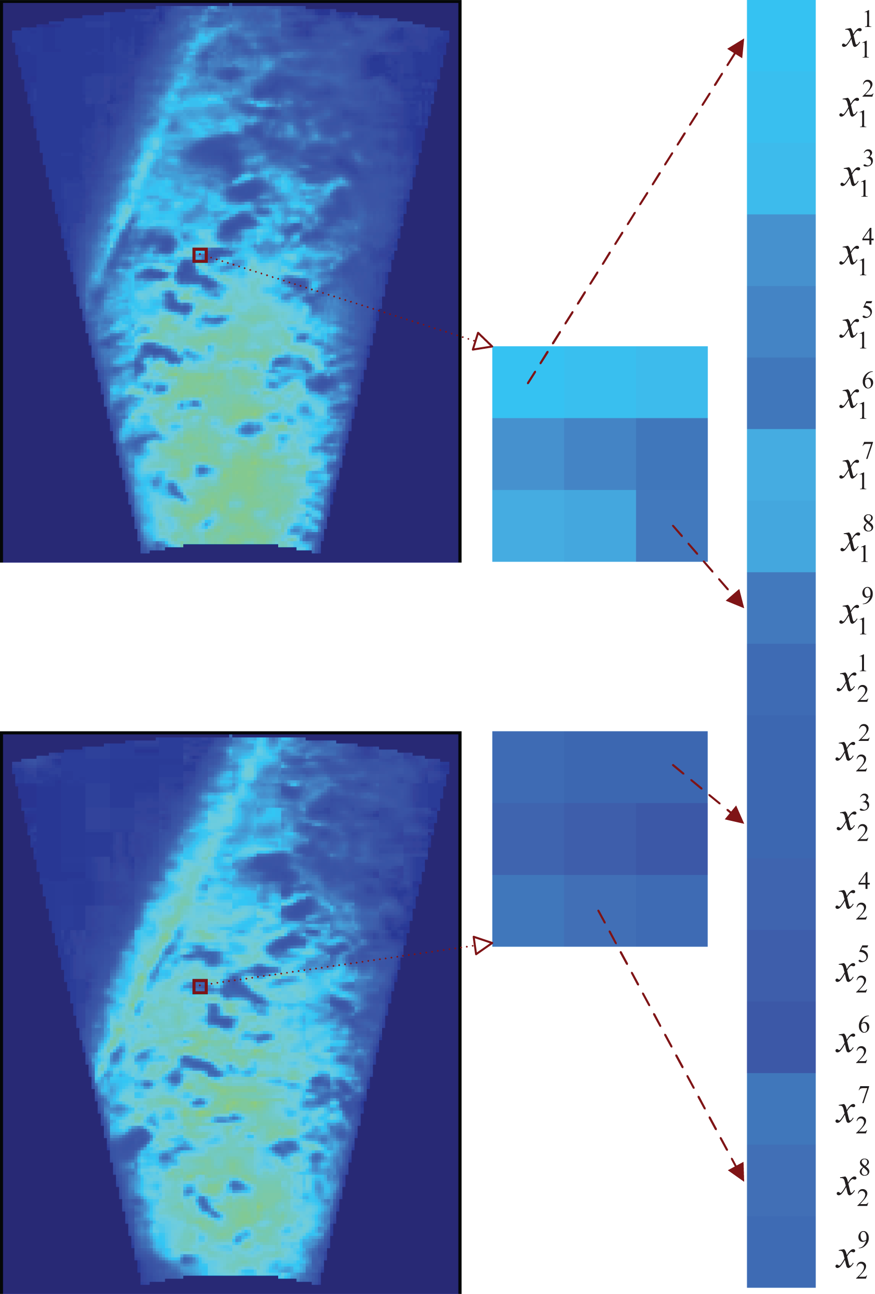Even with a 2D grey–grey image registration, the intensity combination for a single image is 256⁹, and the size of joint histogram is 256¹⁸, such that the joint histogram–based probability calculation scheme is computationally infeasible for multichannel image registration. Consider registering a 2D grey image of N_f = 256 grey levels with a 2D colour image of N_g = 256³ intensity combinations, the size of joint histogram would be $N_{f} \times N_{g} {= 256}^{4}$ . Therefore, it is prerequisite to resort to other feasible methods to calculate the Shannon entropy.

Figure 1.

Concatenation of two corresponding regions to a vector in a row-wise style, which was used by Russakoff et al.²⁵ to calculate the Shannon entropy in a closed form. The pixels are shown in pseudo-colours. Neighbourhood size is 3 × 3.

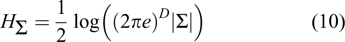
Closed-form solutions for the Shannon entropy are available only in some generic probability distributions, so it makes sense to carry out some approximate discussions. For example, a D-dimensional variable X , which follows a normal distribution with mean μ and covariance Σ

\begin{array}{l} N (X | μ, Σ) \\ = \frac{1}{\sqrt{{(2 π)}^{D} | Σ |}} exp (- \frac{1}{2} {(X - μ)}^{T} Σ^{- 1} (X - μ)) \end{array}

has an analytic entropy³²

H_{Σ} = \frac{1}{2} log ({(2 π e)}^{D} | Σ |)

Substituting equation (10) into (5), the mutual information can be simplified to

I = \frac{1}{2} log (\frac{| Σ_{X_{1}} | | Σ_{X_{2}} |}{| Σ_{(X_{1}, X_{2})} |})

It demonstrates that the calculation of RMI could be largely reduced if the simplified considerations are appropriate for the sonar image. We will discuss it in the next section.

Peripheral mutual information

The multidimensional normal distribution made in equations (9) to (11) is hardly justified, because the data can be seen as a time-shifting serial, then all the dimensions are strongly correlated and almost follow the same distribution. However, the data space could be well accommodated by a multidimensional Gauss distribution if the following two conditions could be satisfied: (i) the data in each dimension are approximately normally distributed and (ii) the different dimensions are independent of each other. The following two subsections are devoted to test and fulfil the conditions.

Normal distribution assumption

The normal distribution assumption can be validated if the intensity histogram of the sonar image can be well-fitted by a single Gauss function.

The histogram can be approximated by a mixture Gauss model (MGM),¹⁵

G (x) = \sum_{k = 1}^{K} \frac{1}{\sqrt{2 π} σ_{k}} exp (- \frac{{(x - μ_{k})}^{2}}{2 σ_{k}^{2}})

where the mixture parameters can be determined by an expectation–maximization algorithm³³ and K is the number of Gauss components. The fitting error is determined by the complexity of the mixture model, with a larger number of Gauss components improving the precision at the cost of computation time. There is no simple way to set the number of Gauss components. Here, it is heuristically determined by the Bayesian information criterion (BIC) rule³⁴

BIC = log (ε^{2}) + Q \frac{log N}{N}

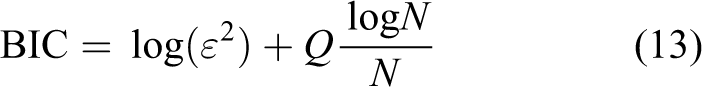
where ε is the fitting error between the intensity histogram and the fitted curve, N is the size of the data, and the parameters number Q = 3K − 1. Note that the multiplication by 3 is in place because there are three parameters for each component, that is, the prior probability, mean and covariance. Subtraction of 1 is because the sum of the prior probabilities is equal to 1.

An example for MGM fitting to the histogram of a sonar image is shown in Figure 2. There is a rapid drop at K = 3 in the BIC curve as shown in Figure 2(b), which demonstrates that the histogram plotted in Figure 2(a) should be described by no more than K = 2 Gauss components. On the other hand, the decrement at K = 2 is so small that the histogram could be approximated by a single Gauss function.

Figure 2.

Quality of the Gaussian approximation for sonar images. (a) The histogram of an image (black solid line) is fitted by a single Gaussian component (red dashed line). (b) The number of Gaussian components is determined by the BIC curve. See the text for details. BIC: Bayes information criterion.

The Gauss function mainly captures the intensity distribution of the background pixels. Note that the largest fitting error appears at around 0.05 (see Figure 2(a)). In fact, such pixels with low intensity are mainly from the shadow areas, which only take a very low proportion in the sonar image when compared with the broad background areas.

It should be noted that the assumption of a normal distribution would be obviously violated if the insonified seabed area does not cover the entire sonar image. The hollow areas before the leading edge or after the trailing edge³⁵ are filled with random noise with an intensity distribution that is very similar to that of the shadow areas. These darker pixels generate a large peak that is different from the one that is generated by the background pixels. Thus, the histogram can no longer be described by a single Gaussian component. Therefore, the scene coverage should be maximized by setting the sonar altitude and grazing angle.

Independence condition

Two variables x and y are independent if the joint probability is equal to the product of the marginal probabilities, $p (x, y) = p (x) p (y)$ . The pixels in a local region are partially dependent on each other, which obviously violates the independence condition.

In statistics, the χ² test can be used to measure the independence between two variables. Now that the variables are not independent, we use the relative value

{\hat{F}}_{i j} = \frac{F_{i j}}{max_{k, l = 1, \dots, D} (F_{k l})}

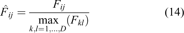
to measure the dependency between variables, where F denotes the basic χ² test value.³⁶

An example for the relative association for neighbouring pixels is shown in Figure 3. The joint intensity distribution between the centre pixel x_(0,0) and a third-order neighbour x_(0,−1) is strongly diagonal (Figure 3(a)), demonstrating strong correlation between the central pixel and its second-order neighbours. The joint distribution of the central pixel and a third-order neighbour x_(−2,−2) is randomly scattered (Figure 3(b)). It demonstrates that the dependence of x_(0,0) on x_(0,−1) is far larger than it on x_(−2,−2). The association values between all the pixels from an image region and its counterpart in another image are shown in Figure 3(c). It can be seen that each pixel is strongly associated with its neighbours, which supports the Markov assumption.^12,30,31

Figure 3.

The association between pixels in the third-order neighbourhood. The joint intensity distribution matrix between $x_{(0, 0)} and x_{(0, - 1)} and x_{(- 2, - 2)}$ are shown in (a) and (b), respectively. (c) The relative χ² test value between all the pixels, which are arranged in a column-wise style. The association matrix is a symmetrical matrix. In the top and right panel of (c), the pixels that are selected to calculate the peripheral mutual information in the third-order neighbourhood are shown in red and marked by ‘2’. (d) Peripheral pixels for different neighbourhood sizes. For pixels of the same neighbourhood, colour and label are the same.

For the third-order neighbours, to reduce the associations between variables as much as possible, only the four peripheral pixels that are located in the corners (refer to the top and right panel of Figure 3(c)) are used to calculate the regional information. Another heuristic strategy, which is also very important for the proposed method, is that the centre pixel is abandoned to further support the independence assumption. Now that the regional information is solely dependent on the outermost pixels, we named it as peripheral mutual information.

The strategy for selecting peripheral pixel applies to different neighbourhood sizes. In Figure 3(d), we display the peripheral pixel configuration for different neighbour radius, that is, r ranges from 1 to 5. Given the radius r, the four pixels that are furthest from the centre pixel, that is, with a block distance 2r, are used to calculate the mutual information.

Algorithm 1.

Peripheral mutual information.

1: Input the floating image f and reference image g, set the neighbour radius r.

2: Initialize the parameter set Θ, set t = 0.

3: while ||ΔΘ|| < ∊ do

4: Transform f to f′ by the current parameter set Θ^(t). To simplify the calculation, the nearest neighbour interpolation method is used to deal with the fractional coordinates.

5: For each pixel s = (r, c), concatenate the four peripheral pixels in the (r + 1)-st order neighbourhood in f′ according to Figure 3(d) to a column vector X ₁. Construct X ₂ with the corresponding pixels in g with the same procedure.

6: Calculate the mutual information I by equation (11).

7: Search a local extreme with Powell’s multidimensional direction set method.

8: Update the parameter set Θ^(t+1) and the direction set.

9: t = t + 1.

10: end while

11: Stitch the image.

The detailed PMI-based sonar image registration method is listed in Algorithm 1. It should be noted that other interpolation strategies may obtain much smoother registration function, but for simplicity, only the simple nearest neighbour method is used in step 4.

Experiments

Two data sets are used to test the performance of the proposed PMI method. Both were collected by a DIDSON sonar when the underwater vehicle operated close to the seabed, where GPS signals are not accessible. Furthermore, the inertial navigation information is unavailable in both cases.

The first data set was taken by the DIV Group ³⁷ with a DIDSON sonar during a pipeline burying mission on the seabed. Screenshots from a screen monitoring the sonar images were compressed into a video stream that lasts 16 s and includes 377 frames. The imaging distance is about 2.5 m.

The second data segment was collected by an autonomous underwater vehicle (AUV) developed by the Center of Marine Information Technology and Equipment, Shenyang Institute of Automation, Chinese Academy of Sciences. The altitude of the AUV was set to be 7 m, which is farther than that of the pipeline burying machine. The elevation angle of the DIDSON sonar is 45° below the horizontal plane. Therefore, the imaging area is about 10 m away from the sonar header. The video shot lasts 10 s and includes 240 frames.

We use four experiments to test the performance of the PMI maximization on sonar image registration. In the first experiment, we try to determine the neighbourhood radius by examining the relationship between the registration function of the proposed PMI and the neighbourhood size. The second experiment is designed to test its feasibility in image registration and examine the smoothing feature of the registration function. The latter two experiments are used to test its performance on the two real image sequences, with the first aiming at a comparison to other methods and the second testing its effectivity for fully unstructured environments.

Neighbourhood size

The inclusion of spatially neighbouring information enhances the robustness of the similarity measure in image registration.²⁵ With increasing neighbourhood radius, the peripheral pixels tend to be randomly distributed, which supports the independence assumption. However, the neighbourhood radius cannot be arbitrarily large, because the mutual information (11) decays with distance. Therefore, an appropriate range for the neighbourhood radius should be determined as a compromise between feasibility of association and suppression of randomness.

In Figure 4, we show the registration functions for a typical sonar image pair matching when the neighbourhood radius r ranges in {0, 1, 2, 3, 9, 15}. Note that for r = 0, the block turns to a single pixel, such that the mutual information depends only on the covariance of a pixel and its counterpart in the other image.

Figure 4.

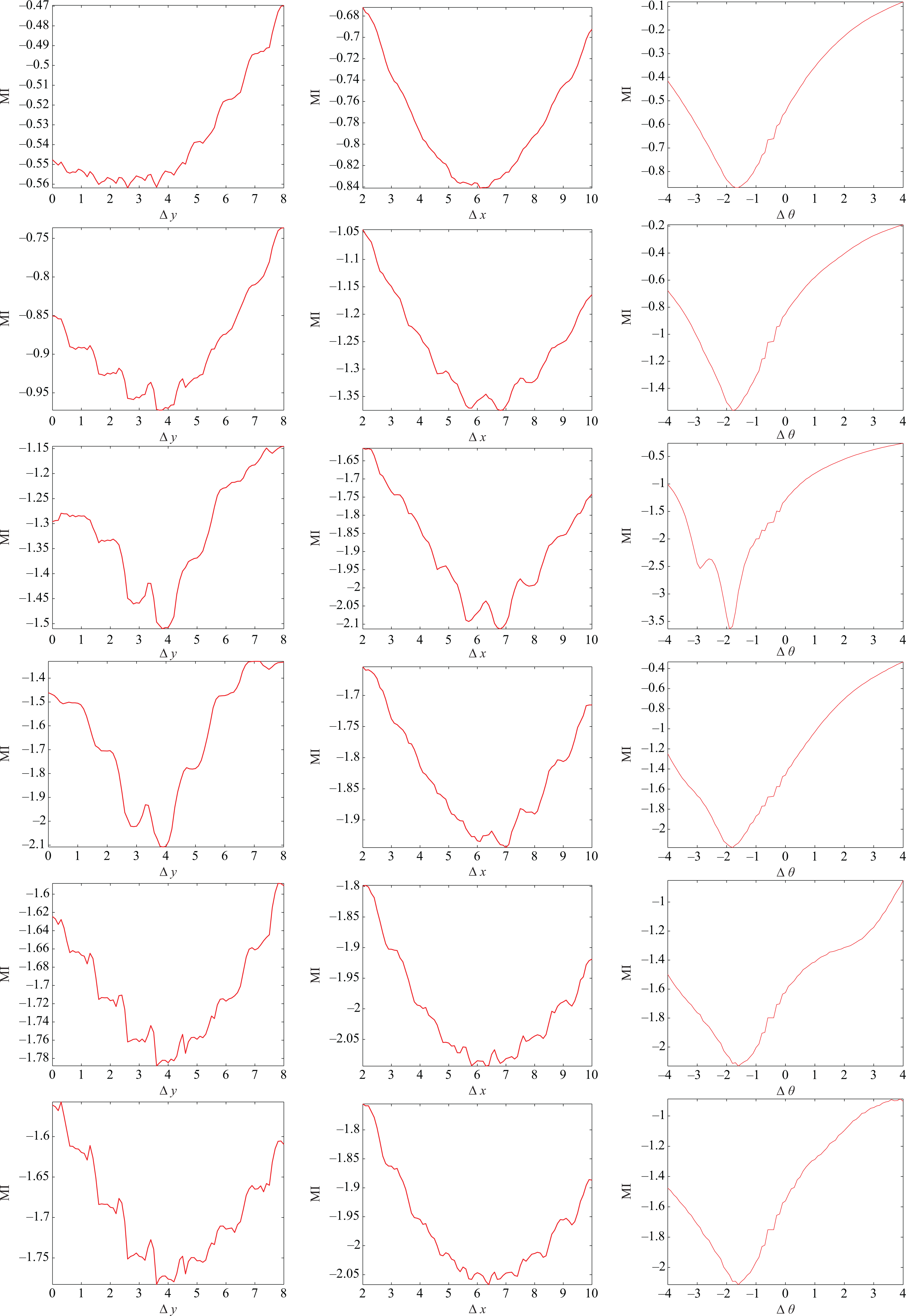
Registration functions with different neighbourhood sizes for a sonar image pair. Left column: translation along vertical and horizontal axis; middle column: translation along horizontal axis; right column: rotation around sonar head. From top to bottom, the neighbourhood radius is r = 0, 1, 2, 3, 9, 15, respectively. Initial parameters are $Δ y = - 1, Δ x = - 2 and Δ θ = 0.5 °$ .

The neighbourhood radius is determined by evaluating the smoothness and the height gap of the registration functions. Though the registration function for r = 0 is smoother than others, no spatial information is included in similarity measure. If r is very large, that is, r = 9 or 15, then large vibrations along the registration function occur. In addition, for large r, many blocks would be discarded due to the boundary effects.

On the other hand, the height gap of the registration functions for r = 2 or r = 3 is far larger than that of others. Take the registration functions displayed in Figure 4 for example. When r = 2 or r = 3, the height gap is $(0.35, 0.45, 3.20) and (0.80, 0.30, 1.80)$ , respectively. However, when r = 0, 1, 9, 15, it drops to $(0.09, 0.16, 0.80), (0.25, 0.33, 1.40), (0.19, 0.30, 1.20) and (0.25, 0.35, 1.15)$ , respectively. A steeper energy boundary tends to increase the convergence speed of the minimization procedure for the mutual information towards local minima. According to our testings and simulations, a better registration precision and a faster convergence speed can be obtained for the mutual information maximization procedure in the case of r = 2. Therefore, in the following experiments, we empirically set the neighbourhood radius to this value.

Estimate the known sonar image pairs

Because of the missing inertial navigation information, it is impossible for us to evaluate the motion parameters that are estimated from the image pairs by comparing them with the physical movement of the underwater vehicle. Instead, an alternative scheme, where the floating image is transformed from the reference image with a known parameter set, is proposed to test the precision of the proposed sonar image registration method. In total, 137 sonar frames are randomly selected from the videos as the reference images. Each frame is transformed into 9 floating images with a randomly generated parameter set which provides us with 1233 sonar image pairs. Then, we use several methods to estimate the transformation parameters, including PV-based mutual information²² and its revisions that include the gradient information (gradPV),²³ GPVE,²⁴ RMI²⁵ and the proposed PMI. To test whether RMI is feasible for higher-order neighbourhoods, we set the neighbourhood radius r to 1 and 2 and checked the estimation precision. The parameters are all initialized by zeros.

To narrow down the search range, the maximum horizontal and vertical translation parameters are limited to 10 pixels, that is, $Δ x, Δ y \in [- 10, 10]$ . The maximum rotation angle is also limited to 10°, that is, $Δ θ \in [- 10 °,10 °]$ . It is worth mentioning that a multi-resolution procedure would be appropriate for the optimization procedure if it has to be assumed that the translation and the rotation parameters exceed these values.

Precision

Powell’s search method is used to prevent the mutual information becoming trapped in local minima. The precision of the parameter estimation is largely determined by the robustness of the search method. In essence, Powell’s method tries to accelerate the converging speed by constructing a set of conjugate directions, which is further determined by the local minimum that is reached with the current direction set.

To search for local minima in every direction, we use Brent’s one-dimensional line minimization procedure. It is based on parabola-shaped pitfalls that reside in $[Θ_{0}, Θ_{2}]$ along each direction and which have to be located at first. This implies that we have to find three points $Θ_{0}, Θ_{1} = Θ_{0} + η_{1} d V and Θ_{2} = Θ_{1} + η_{2} d V$ along the direction dV, such that $M I (Θ_{0}) \geq M I (Θ_{1}) and M I (Θ_{2}) \geq M I (Θ_{1})$ , where η₁ and η₂ are two constants determined by the searching procedure. However, there are many local minima along the registration curves (see Figure 5). A strategy is adopted to help the mutual information escape the local minima. The searching step will continue if $M I (Θ_{2}) \geq (1 + ε) M I (Θ_{1}) and max_{j = 1, 2, 3} (Θ_{1}^{j} - Θ_{2}^{j}) < 10$ , where ε is set to be 0.05 empirically, the superscript j stands for the dimension.

Figure 5.

Registration functions for a sonar image pair. Left column: translation along vertical and horizontal axis; middle column: translation along horizontal axis; right column: rotation around the sonar head. From top to bottom: PV, gradPV, GPVE, RMI (r = 1), RMI (r = 2) and PMI. Initial parameters are $Δ y = - 1, Δ x = - 2 and Δ θ = 0.5$ . gradPV: gradient information; GPVE: generalized partial volume estimation; RMI: regional mutual information; PMI: peripheral mutual information; PV: trilinear partial volume distribution.

An example for motion parameters estimation is presented in Table 1. It can be seen that the proposed PMI method and the GPVE method are more accurate than other methods. The average estimation precision for each method is displayed in Table 2.

Table 1.

Estimate motion parameters for a known sonar image pair with different mutual information methods.

Estimation	True parameters	PV	Gradient + PV	GPVE	RMI (r = 1)	RMI (r = 2)	PMI (d = 2)
Δy	−2	−2.0466	−2.9957	−2.0230	−2.9957	−3.2853	−2.0041
Δx	5	4.4669	5.0072	4.8955	5.0072	1.9386	4.8881
Δθ	5	4.7356	4.9835	4.9839	4.9835	4.9721	4.9836

GPVE: generalized partial volume estimation; PV: trilinear partial volume distribution; RMI: regional mutual information; PMI: peripheral mutual information.

Table 2.

Average estimation error for different mutual information methods.

Error	Δy	Δx	Δθ
PV	0.1868 ± 0.5183	−;0.6906 ± 1.6265	−;0.2060 ± 0.4404
Gradient + PV	−;0.0267 ± 0.5758	−;2.1243 ± 4.2030	−;0.5648 ± 1.1404
GPVE	−;0.0146 ± 0.0168	−;0.0187 ± 0.0955	−;0.0026 ± 0.0239
RMI (r = 1)	−;0.1994 ± 0.9072	0.2855 ± 1.5136	−;0.0388 ± 0.2909
RMI (r = 2)	−;0.1641 ± 2.2336	−;0.1571 ± 2.4954	−;0.0329 ± 0.1228
PMI (d = 2)	−;0.0048 ± 0.0298	0.0670 ± 0.1887	0.0294 ± 0.0486

GPVE: generalized partial volume estimation; PV: trilinear partial volume distribution; RMI: regional mutual information; PMI: peripheral mutual information.

Three conclusions can be drawn at this point. Firstly, GPVE obtains best performance in the methods that depend on the histogram and interpolation, while the proposed PMI method performs best in the RMI methods. PMI is comparable to the GPVE method as both use mean error and variance. However, as discussed above, the main advantage of RMI is its ability to register high-dimensional data without the histogram calculation and pixel interpolation. Secondly, the estimation results for RMI (r = 2) are almost catastrophic, which demonstrate that it is inappropriate to incorporate a second-order neighbourhood into RMI. Thirdly, there is a larger improvement in the estimation precision of PMI over RMI. Though a large effort should be made to the RMI, the initial experiment tells that an appropriate neighbour selection strategy is helpful for the mutual information calculation.

There is a further problem related to precision. Even the best method (GPVE here) occasionally has a large bias (data not shown). It is perhaps due to the speckle noise which affects acoustic echoes and weakens the correlation between corresponding pixels.

Registration function

It is necessary to analyse the mechanism that underlies the mutual information maximization by examining the registration function of different methods. For example, a floating sonar image f is transformed from the reference image g with a known parameter set Θ = {1, −2, −1}, the dimensions of which correspond to Δy, Δx and Δθ, respectively.

The estimation results are listed in Table 1. For the registration methods that are based on mutual information, the opportunity to find the global optimum is largely determined by the registration function. Therefore, those methods that derive the joint and marginal probabilities from the joint histogram have tried to construct a smoother registration function by different kinds of heuristic strategies in pixel interpolation.^22
–24,27 However, the RMI methods, that is, RMI and the proposed PMI, directly incorporate the neighbouring information into the mutual information by a closed-form approximation to the Gauss–Shannon entropy. It is necessary to check that if the registration function in the RMI methods also has a smooth registration function, because all the methods depend on the same optimization procedures.

In Figure 5, we plot the registration functions when translation and rotation happen. The initial parameter setting is Θ = {−1, −2, 0.5}. The three columns, from left to right, represent the horizontal translation, the lateral translation and the rotation around the vertical axis, respectively. Each row corresponds to the registration functions of a special method. Three conclusions can be drawn from Figure 5.

Firstly, there are many local minima in the translation dimensions (see the first row to the third row in Figure 5) for the histogram-based methods. In the absence of the rotation, the interpolation is equivalent to the reallocation of weights, leading to a temporary increase in mutual information. However, the dithering effects are suppressed by the step effects of the RMI methods, because all the weights jump between 0 and 1 synchronously in the case of nearest neighbour interpolation. That is, the mutual information keeps fixed for fractional translation. When the robot makes a turn, the step effects in the registration functions of RMI and PMI disappear, because the synchronism no longer exists. The step effects of RMI (r = 2) aggravate to the sawtooth effects, which show again that the second-order neighbourhood is a tragedy for the RMI.

Secondly, the registration function of RMI (r = 2) does not behave as a pitfall (see the fifth row of Figure 5), which demonstrates that the second-order neighbourhood is inappropriate for the RMI.

Lastly, the registration function of the proposed PMI has a very steep valley, which indicates that the proposed PMI method has the potential to converge with a faster speed. Indeed, PMI converges in three to five iterations in our simulations.

Fourthly, it is astonishing to find that the registration curve of PMI is not only far smoother than that of RMI but also comparable to that of GPVE. Recall that GPVE makes use of luxury spline interpolation to extend the neighbourhood and construct the joint histogram, whereas PMI only depends on the simple nearest neighbour interpolation. It indicates that the peripheral pixels are sufficient to measure the mutual information on one hand. On the other hand, the PMI method has the potential to obtain a comparative registration performance with the traditional histogram-based methods.

Lastly, the sawtooth effects in the registration function gradPV (second row in Figure 5) show that the gradPV is an incredible feature for the underwater sonar image.

It is worthy to note that there are local minima along the registration curves. A small perturbation will help the mutual information escape the local minima. On the other hand, the motion information from other sensors, like the odometer, will surely help the optimization procedure find the optimum more quickly.

Sonar image registration (1): Pipeline burying

In this experiment, we try to register the sonar frames from the pipeline burying data set with different methods. The data were collected when the underwater vehicle was laying the pipeline on the seabed. To reduce the computation cost, the registration starts only when the average intensity difference between the two images exceeds a threshold T. We have chosen the value T = 0.02. The only exception is NDT, where T = 0.01, because the gradient descent method is inappropriate for estimating the larger motion parameters.

Experimental setting

According to the first experiment, the third-order neighbourhood (r = 2) is inappropriate for the RMI method and the gradPV should be abandoned for sonar images. Therefore, among the mutual information methods that are discussed above, only the PV, GPVE, RMI (r = 1) and PMI are selected for evaluation in the current simulations.

On the other hand, as described in the Introduction, the NDT method and the FMT method have been adopted by Aykin and Negahdaripour¹⁴ and Hurtós,^18,20 respectively, to register 2D forward-looking sonar images. Further, the SIFT feature points³⁸ have been widely accepted as the most robust and discriminative features for the images that are taken in the structured or semi-structured environment,²¹ such as the seabed working range. Therefore, it is necessary to compare the performance of the proposed PMI method with FMT, NDT and SIFT-based image matching methods.

For the FMT method, we strictly follow the method suggested by Hurtós et al.²⁰ to register the sonar images. The rotation angle is estimated by locating the maximum of the phase correlation matrix between f and g in polar coordinates, while the translation parameters are estimated by locating the maximum of the phase correlation matrix between the angle-compensated floating image f_θ and the reference image g in Cartesian coordinates. Note that the histogram equalization is adopted to enhance the high-frequency information.

To apply the NDT method, a preprocessing procedure that is similar to the one suggested by Aykin and Negahdaripour¹⁴ has been designed to extract the feature areas. Because the shadows are often the most salient and robust features in underwater sonar images, we extract the shadow areas as the candidate blobs with the method described by Hsieh et al.³⁹ For concave shadow blobs that cannot be modelled appropriately by a Gauss distribution, a clump splitting method⁴⁰ is adopted to segment them into convex sub-blocks.

The SIFT feature points are extracted by the code provided by Lowe.⁴¹

Comparison between mutual information methods

The image registration performances between different mutual information methods are compared at first.

Initially, the local immediate registration error is evaluated by registering an image pair. The results are shown in the top row of Figure 6(a) to (d). The two original images are shown in red and green, respectively. Therefore, the perfectly aligned pixels appear in yellow. It is convenient to qualitatively compare their performance by observing the proportion of red or green pixels in the overlapping region, especially along the edges of objects or shadows. It can be seen that the proposed PMI has a very similar performance as that of the GPVE method. Both of them are superior to the PV and RMI (r = 1) methods.

Figure 6.

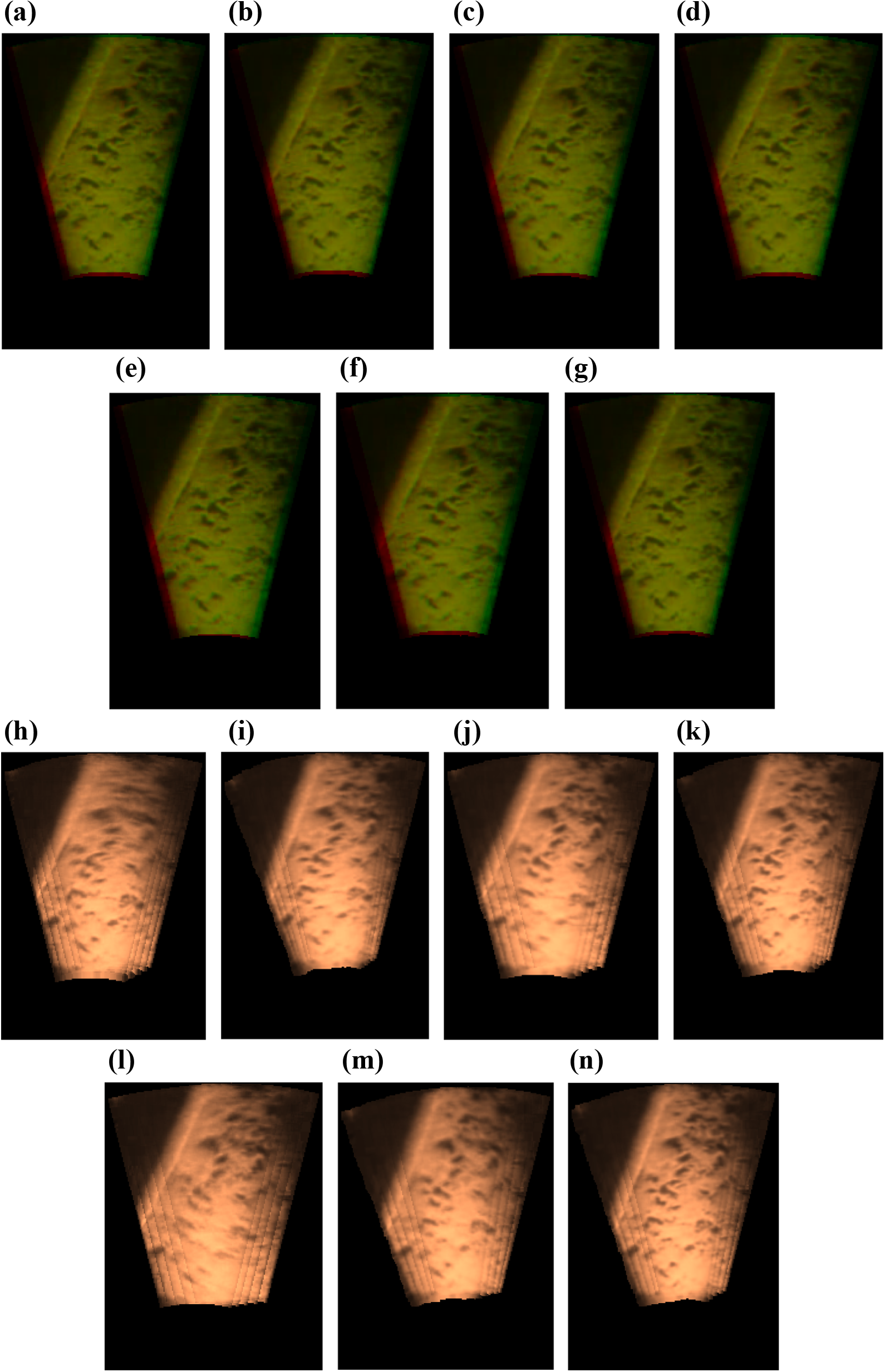
Registration of a sonar image sequence with the mutual information methods. For the first and the third row, from left to right, the columns correspond to PV, GPVE, RMI (r = 1) and PMI, respectively. For the second row and the bottom row, the columns correspond to FMT, NDT and SIFT, respectively. The image pair registration (#01 and #21) is shown in the top two rows, where the two images are shown in red and green, respectively, and the correct alignment is shown in yellow. The accumulated error is observed by registering five consecutive frames in the bottom two rows. Note that 12 frames are used in the NDT method, see text for details. Global error adjustment is outside the scope of this article. GPVE: generalized partial volume estimation; RMI: regional mutual information; PMI: peripheral mutual information; PV: trilinear partial volume distribution; FMT: Fourier–Mellin transform; NDT: normal distribution transform; SIFT: scale-invariant feature transform.

The differences between the estimated registration parameters between different methods are so small that it is very hard to evaluate the performance by the immediate error. Local registration errors will be accumulated rapidly if consecutive frames are registered to form a panoramic view. The panoramic image soon becomes blurred if the local error is very large. Therefore, the registration precision can be observed by watching the edges and details in the global image.

In the third row of Figure 6 (from Figure 6(h) to (k)), we show the panoramic images when five consecutive frames are registered. It can be seen that the top half of the panoramic image that is generated by the PV method is so blurred that it turns to a uniform region. A large number of details are lost in the averaging step. Intuitively, PMI and GPVE almost have an equivalent performance.

The residual error, which is defined as the mean energy difference between the transformed floating image f_Θ* and the reference image g in the overlapping area O

r = \frac{1}{‖ O ‖} \sum_{(i, j) \in O} | f_{Θ^{*}} (i, j) - g (i, j) |

is adopted to describe the registration precision, where ‖O‖ is the pixel number in the overlapping area.

The residual errors between the five sequential sonar frames are displayed in Table 3. It can be seen that the proposed PMI method is even better than the GPVE method in the estimation precision. It is indeed that the bottom half of Figure 6(k) has clearer edge information and preserves more details compared to Figure 6(i).

Table 3.

Residual errors for the image sequence registration in Figure 6.

Residual	PV	GPVE	RMI (r = 1)	PMI	FMT	NDT	SIFT
(#01, #21)	0.0297	0.0266	0.0275	0.0251	0.0323	0.0360	0.0246
(#21, #32)	0.0367	0.0342	0.0388	0.0309	0.0572	0.0380	0.0321
(#32, #40)	0.0393	0.0452	0.0416	0.0276	0.0386	0.0378	0.0289
(#40, #49)	0.0314	0.0311	0.0330	0.0297	0.0410	0.0306	0.0298
Average	0.0343	0.0343	0.0352	0.0283	0.0423	0.0356	0.0289

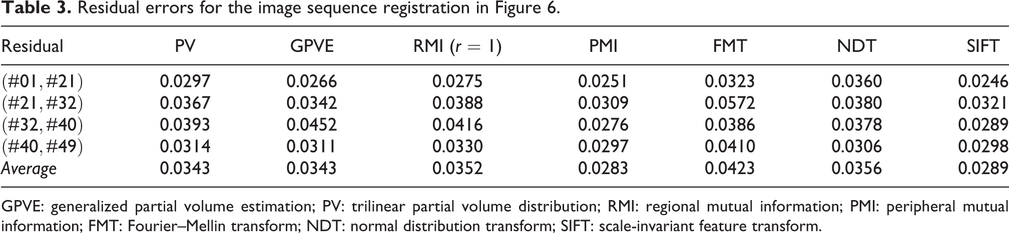
GPVE: generalized partial volume estimation; PV: trilinear partial volume distribution; RMI: regional mutual information; PMI: peripheral mutual information; FMT: Fourier–Mellin transform; NDT: normal distribution transform; SIFT: scale-invariant feature transform.

Comparison to other methods

Finally, we show the results obtained by the FMT, NDT and SIFT-based methods. The sonar image pair registration results are shown in Figure 6(e) to (g) (second row), and the consecutive image sequence stitching results are shown in Figure 6(l) to (n) (bottom).

The proposed PMI method has a performance comparative to the SIFT-based method. However, the SIFT feature point extraction algorithm is feasible for image registration only when there is clear, high-frequency information. As discussed by Negahdaripour et al.,¹¹ such information is absent in many natural environments.

The precision of FMT depends on the resolution of the sonar image. The size and resolution of the sonar frames in the pipeline burying data set is far lower than the practical DIDSON sonar image. When calculating the rotation angle in the polar coordinates, the error that is related to a single pixel is about 2 degrees, leading to the rapid growth of the accumulated error. A subpixel estimation is helpful for controlling the registration error; however, it is limited to translation effects at present.⁴²

NDT pursues the local minima by the computation-exhaustive gradient descent method, which might impede its application in the practical engineering. At first, NDT has a tendency towards underestimation, because the Gauss model is able to smooth the contour of each blob, which is more appropriate to describe the motion tendency approximately. Secondly, since NDT is optimized by the Gauss–Newton gradient descent strategy,⁴³ it relies on an inverse of the Hessian matrix which may cause instability in the optimization process, which is hardly alleviated by the Levenberg–Marquardt method.⁴⁴ Therefore, it is unlikely that NDT converges to the global minimum. Thirdly, NDT is computationally expensive, because a normal distribution distance has to be calculated for each pixel in each iteration. Lastly, it is nontrivial to choose an appropriate learning rate. With a smaller learning rate, it would take a very long time for the optimization procedure to converge to the local minima. Inverse, a larger learning rate is very likely to bring in oscillations to the iteration steps.⁴⁵

Sonar image registration (2): Unstructured environment

The pipeline burying field can be seen as a structured environment, where abundant corner points, edges or shadow blobs could be extracted to support the feature matching. However, such a flourishing situation seldom happens on the natural sea floor. On the other hand, a large number of local features would be invisible if the object is far away from the sonar header. In Figure 7(g), we show two sequential sonar frames from the second data set, which are taken from the natural seabed with an imaging distance of 9 m. Only three SIFT feature point pairs could be extracted using the code provided by Lowe,⁴¹ leading to an underdetermined system of equations that is infeasible for the motion parameters estimation. Such a dilemma is hardly alleviated even if we remove the Gaussian noise with a median filter in the preprocessing stage.

Figure 7.

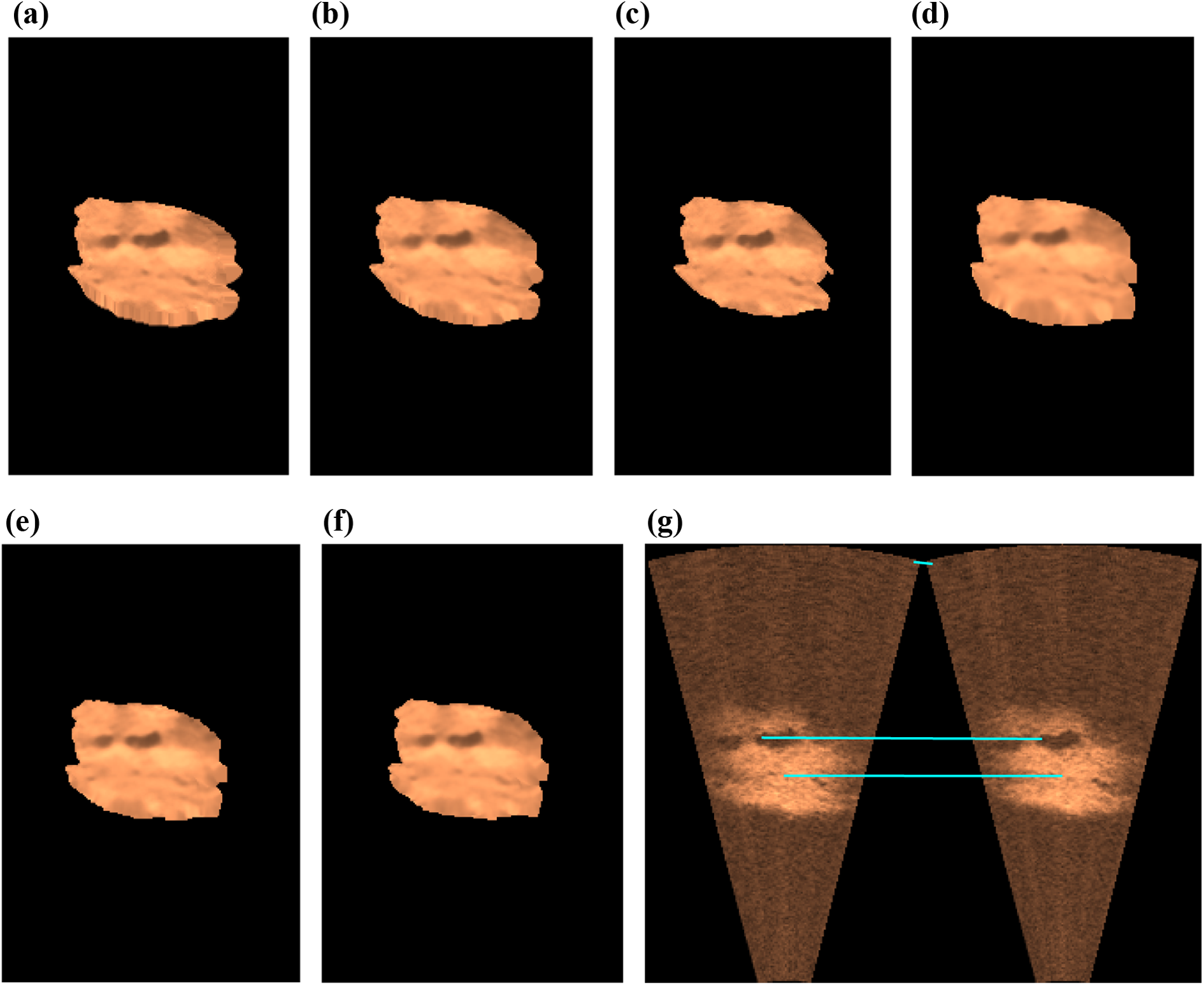
Registration of 10 sequential sonar frames that are acquired from a natural sea floor. (a) to (f) Correspond to PV, GPVE, RMI (r = 1), PMI, FMT and NDT, respectively. SIFT method is infeasible here, because too few feature points were identified. For example, only three SIFT feature point pairs could be extracted in (g). Note that the seabed is 9 m away from the sonar header. For simplicity, only the illuminated area is considered for registration. GPVE: generalized partial volume estimation; RMI: regional mutual information; PMI: peripheral mutual information; PV: trilinear partial volume distribution; FMT: Fourier–Mellin transform; NDT: normal distribution transform; SIFT: scale-invariant feature transform.

It is only necessary for us to register the illuminated area because it takes up a very small part of the whole sonar frame. The region of interest can be obtained by segmenting the average illumination pattern with an appropriate threshold.¹⁹ The stitching results of 10 consecutive sonar frames for the PV, GPVE, RMI (r = 1), PMI, FMT and NDT methods are displayed in Figure 7(a) to (f), respectively. The corresponding residual errors are shown in Table 4.

Table 4.

Residual errors for the image sequence registration in Figure 7.

Methods	PV	GPVE	RMI (r = 1)	PMI	FMT	NDT	SIFT
Average error	0.0356	0.0347	0.0348	0.0341	0.0359	0.0356	–

There is no significant difference in the residual error between the proposed PMI method and other methods that are based on mutual information maximization. The underlying reason may be that the sonar frame is dominated by the background pixels. The slight change in motion parameter is not able to bring in the remarkable variation in the mutual information. The fact also explains that though the residual error of PMI is smaller than other methods, the panoramic image shown in Figure 7(d) appears more blurred than others.

Unstructured environment also challenges the application of the FMT and NDT methods. The faintness in the high frequency information, which is mainly generated by the sparse and blurred edges, degrades the impulse intensity in the Fourier domain or the Fourier log-magnitude domain, hindering the precise location of the translation and rotation parameters with the FMT method (Figure 7(e)).

To some extent, the precision of NDT depends on the blob extraction methods. Similarly, the slight change in the insonification pattern and incidence angle brings large uncertainties in the region boundaries, bringing huge disturbance to the normal distribution modelling and the sequential optimization procedure. Comparing Figure 7(f) and Figure 6(m), it can be seen that the motion parameters can be better estimated if there are a large number of feature areas in the case of blurred images.

Conclusion

In this article, we propose the PMI method for registering 2D forward-looking sonar images. PMI is inspired by RMI but differs in that only the outermost neighbours are used to calculate the Gaussian–Shannon entropy. The method provides an improved solution for the sonar image registration problem, where RMI cannot be applied for the higher order neighbourhoods due to the violation of normal distribution assumption.

Our experimental results illustrate that PMI not only behaves better than the RMI method but also has a performance that is superior to the traditional histogram-based mutual information methods. Furthermore, PMI is attractive in several other aspects:

Firstly, PMI calculates the mutual information with a closed-form solution that depends only on the covariance matrix between pixels. This means that there is no need to construct a joint intensity histogram, reducing memory requirements of the algorithm. On the other hand, PMI only needs to calculate the covariance matrix with the outermost neighbours, largely reducing the computation costs.

Secondly, PMI does not require an elaborate interpolation function, because even the simple nearest-neighbour interpolation method is able to obtain a smoother registration function.

Thirdly, PMI has a smoother registration function, which means that it is largely possible to converge to global optimum. Furthermore, the gradient around the local minimum in the registration function of PMI is very steep, which means that it is able to converge with a faster speed.

Lastly, PMI can be used to register cross-dimension sensor data, which is the incentive of designing the RMI methods. Theoretically speaking, it is possible to register data with any dimensions, because PMI executes in a very simple mode: extracts the peripheral pixels of an image region and its counterpart in another image, calculating the covariance matrix and the Gauss–Shannon entropy. A work on acousto-optic image registration will be reported in the near future.

Underwater sonar image is prone to speckle noise, which indicates that it lacks the general high-frequency information. Mutual information maximization provides us with a method to register the images that are sampled from the fully unstructured underwater environment. Two aspects will be focused in the next step. On the one hand, we will try to find a better optimization strategy for PMI to increase its robustness and registration precision. On the other hand, we will try to reduce the accumulated error in the framework of mutual information.

Footnotes

Acknowledgements

The authors are grateful to Kexin Zhu from DIV Group (Shenzhen) for sharing the sonar data and to the anonymous reviewers for their valuable comments on the previous versions of the article.

Declaration of conflicting interests

The authors declared no potential conflicts of interest with respect to the research, authorship, and/or publication of this article.

Funding

The authors disclosed receipt of the following financial support for the research, authorship, and/or publication of this article: The work is supported by the National Natural Science Foundation of China (no. 41506121), the National Key Research and Development Program of China (no. 2016YFC0300801, no. 2016YFC0300604, no. 2016YFC0301601), the National High-Tech Research and Development Program of China (no. 2014AA09A110), the Instrument Developing Project of the Chinese Academy of Sciences (no. YZ201441), the Strategic Priority Program of the Chinese Academy of Sciences (no. XDA13030203), the Youth Innovation Promotion Association CAS (no. 2011161), the Distinguished Young Scholar Project of the Thousand Talents Program of China (no. Y5A1370101), the State Key Laboratory of Robotics of China (no. 2017-Z010, No. Y5A1203901), the Natural Science Foundation of Jiangsu Province, China (no. BK20170558), the project of ‘R&D Center for Underwater Construction Robotics’, funded by the Ministry of Ocean and Fisheries (MOF) and Korea Institute of Marine Science & Technology Promotion (KIMST), Korea (No. PJT200539) and the Public science and technology research funds projects of ocean (no. 201505017).

References

Tian

. Integrated method for the detection and location of underwater pipelines. Appl Acoustic 2008; 69(5): 387–398.

Jacobi

Karimanzira

. Underwater pipeline and cable inspection using autonomous underwater vehicles. In: OCEANS-Bergen, Bergen, Norway, 11–14 June 2013, pp. 1–6. MTS/IEEE.

Song

Herrmann

Liu

. Forward-looking sonar image mosaicking by feature tracking. In: Robotics and Biomimetics (ROBIO), 2016 IEEE International Conference, Qingdao, China, 3–7 December 2015, pp. 1613–1618. IEEE.

Zou

Bian

Chang

. A real-time obstacle avoidance method for AUV using a multibeam forward looking sonar. ROBOT Chin 2007; 29(1): 82–87.

Tao

Lin

Guo

. First active hydrothermal vents on an ultraslow-spreading center: Southwest Indian ridge. Geology 2012; 40(1): 47–50.

Ozog

Troni

Kaess

. Building 3D mosaics from an autonomous underwater vehicle, doppler velocity log, and 2D imaging sonar. In: Robotics and Automation (ICRA), 2015 IEEE International Conference, Seattle, Washington, 26–30 May 2015, pp. 1137–1143. IEEE.

Brown

Lowe

. Automatic panoramic image stitching using invariant features. Int J Comput Vis 2007; 74(1): 59–73.

Zhu

. A coarse-to-fine scheme for groupwise registration of multisensor images. Int J Adv Robot Syst 2016; 13(6): 1–12. DOI: 10.1177/1729881416673302.

Negahdaripour

Firoozfam

Sabzmeydani

. On processing and registration of forward-scan acoustic video imagery. In: Computer and Robot Vision, 2005. Proceedings. The 2nd Canadian Conference, Victoria, BC, Canada, 9–11 May 2005, pp. 452–459. IEEE.

10.

Kim

Neretti

Intrator

. Mosaicing of acoustic camera images. IEE Proc Radar, Sonar Navig 2005; 152(4): 263–270.

11.

Negahdaripour

Aykin

Sinnarajah

. Dynamic scene analysis and mosaicing of benthic habitats by FS sonar imaging – issues and complexities. In: Oceans 2011, Kona, Hawaii, 19–22 September 2011, pp. 1–7. IEEE.

12.

Song

Bailu

Herrmann

. Local autoencoding for parameter estimation in a Hidden Potts-Markov random field. IEEE Trans Image Proc 2016; 25(5): 2324–2336.

13.

Johannsson

Kaess

Englot

. Imaging sonar-aided navigation for autonomous underwater harbor surveillance. In: Intelligent Robots and Systems (IROS), 2010 IEEE/RSJ International Conference, Taipei, China, 18–22 October 2010, pp. 4396–4403. IEEE.

14.

Aykin

Negahdaripour

. Fourier-based registration for robust forward-looking sonar mosaicing in low-visibility underwater environments. J Field Robot 2013; 30(4): 602–623.

15.

Duda

Hart

Stork

. Pattern Classification /. New York: Wiley, 2001.

16.

Casasent

Psaltis

. Position, rotation, and scale invariant optical correlation. Appl Opt 1976; 15(7): 1795–9.

17.

Reddy

Chatterji

. An FFT-based technique for translation, rotation, and scale-invariant image registration. IEEE Trans Image Proc 1996; 5(8): 1266–1271.

18.

Hurtós

Petillot

Salvi

. Fourier-based registrations for two-dimensional forward-looking sonar image mosaicing. In: Intelligent Robots and Systems (IROS), 2012 IEEE/RSJ International Conference, Vilamoura, Algarve, Portugal, 7–12 October 2012, pp. 5298–5305. IEEE.

19.

Hurtós

Cufi

Salvi

. A novel blending technique for two-dimensional forward-looking sonar mosaicing. In: Oceans-San Diego, California, 22–28 September 2013, pp. 1–7. IEEE.

20.

Hurtós

Cufí

Petillot

. Fourier-based registration for robust forward-looking sonar mosaicing in low-visibility underwater environments. J Field Robot 2015; 32(1): 123–151.

21.

Luo

Huang

. An adaptive image-stitching algorithm for an underwater monitoring system. Int J Adv Robot Syst 2014; 11(166): 1–9. DOI: 10.5772/58988.

22.

Maes

Collignon

Vandermeulen

. Multimodality image registration by maximization of mutual information. IEEE Trans Med Imaging 1997; 16(2): 187–198.

23.

Pluim

Maintz

Viergever

. Image registration by maximization of combined mutual information and gradient information. IEEE Trans Med Imaging 2000; 19(8): 809–814.

24.

Chen

Varshney

. Mutual information-based CT-MR brain image registration using generalized partial volume joint histogram estimation. IEEE Trans Med Imaging 2003; 22(9): 1111–1119.

25.

Russakoff

Tomasi

Rohlfing

. Image similarity using mutual information of regions. In: Computer vision - ECCV 2004, European conference on computer vision proceedings, Prague, Czech Republic, 11–14 May 2004, pp. 596–607. Springer Berlin Heidelberg.

26.

Woods

Mazziotta

Cherry

. MRI-PET registration with automated algorithm. J Comput Assist Tomogr 1993; 17(4): 536–546.

27.

Zhang

. Mutual information-based multimodal image registration using a novel joint histogram estimation. Comput Med Imaging Graph 2008; 32(3): 202–209.

28.

Zhao

. Medical image registration based on feature points and Rényi mutual information. Chin J Comput 2015; 38(6): 1212–1221.

29.

Voronov

Tashlinskii

. Efficiency analysis of information theoretic measures in image registration. Pattern Recognit Image Anal 2016; 26(3): 502–505.

30.

Song

Feng

. Prior parameter estimation for Ising-MRF-based sonar image segmentation by local center-encoding. In: OCEANS 2015-Genova, Genova, Italy, 18–21 May 2015, pp. 1–5. IEEE.

31.

Song

Feng

. Label field initialization for MRF-based sonar image segmentation by selective autoencoding. In: OCEANS 2016-Shanghai, Shanghai, China, 10–13 April 2016, pp. 1–5. IEEE.

32.

Shannon

. A mathematical theory of communication. Mobile Comput Commun Rev 2001; 5(1): 3–55.

33.

Dempster

Laird

Rubin

. Maximum likelihood from incomplete data via the EM algorithm. J Royal Statist Soc Ser B Methodol 1977; 39(1): 1–38.

34.

Fraley

Raftery

. How many clusters? Which clustering method? Answers via model-based cluster analysis. Comput J 1998; 41(8): 578–588.

35.

Negaharipour

. On 3-D scene interpretation from FS sonar imagery. In: Oceans, Hampton Roads, Virginia, 14–19 October 2012, pp. 1–9. IEEE.

36.

Hogg

Craig

. Introduction to Mathematical Statistics, 5th ed. Upper Saddle River, New Jersey: Prentice Hall, 1995.

37.

Div iving engineering co., ltd. http://www.drsubsea.com/index_en.html (accessed 30 May 2017).

38.

Lowe

. Distinctive image features from scale-invariant keypoints. Int J Comput Vis 2004; 60(2): 91–110.

39.

Hsieh

Olsonbaker

Fox

. A screening application for image data collected by an acoustic lens sonar Report no. APL-UW-TR-0502, 2005; Washington: Washington Univ Seattle Applied Physics Lab.

40.

Wang

Zhang

Ray

. Clump splitting via bottleneck detection and shape classification. Pattern Recognit 2012; 45(7): 2780–2787.

41.

Lowe

. Demo software: Sift keypoint detector. http://www.cs.ubc.ca/~lowe/keypoints/ (accessed 10 February 2017).

42.

Foroosh

Zerubia

Berthod

. Extension of phase correlation to subpixel registration. IEEE Trans Image Proc 2002; 11(3): 188–200.

43.

Biber

Straßer

. The normal distributions transform: a new approach to laser scan matching. In: Intelligent Robots and Systems, 2003. (IROS 2003). Proceedings. 2003 IEEE/RSJ International Conference, Las Vegas, USA, 27–31 October 2003, pp. 2743–2748. IEEE.

44.

Press

Flannery

Teukolsky

. In Numerical Receipts in C: The Art of Scientific Computing. 2nd ed. Cambridge, UK: Cambridge University Press, 1992.

45.

Haykin

. Neural Networks: A Comprehensive Foundation, 3rd ed. Upper Saddle River, NJ, USA: Prentice-Hall, Inc., 2007.

Two-dimensional forward-looking sonar image registration by maximization of peripheral mutual information

Abstract

Keywords

Introduction

Methodology

Overview of mutual information

State of the art

Regional mutual information

Peripheral mutual information

Normal distribution assumption

Independence condition

Experiments

Neighbourhood size

Estimate the known sonar image pairs

Precision

Registration function

Sonar image registration (1): Pipeline burying

Experimental setting

Comparison between mutual information methods

Comparison to other methods

Sonar image registration (2): Unstructured environment

Conclusion

Footnotes

Acknowledgements

Declaration of conflicting interests

Funding

References