Sage Journals: Discover world-class research

Abstract

Autonomous vehicles are considered to have great potentials in improving transportation safety and efficiency. Autonomous follow driving is one of the highly probable application forms of autonomous vehicles in the near future. In this article, we aim at the basic autonomous following form with one follower and one leader. Proper longitudinal regulation of the follower vehicle is essential for the driving quality of the two-vehicle platoon. Focusing on this problem, a novel longitudinal control method composing of a learning-based acceleration decision phase and an internal model–based acceleration tracking phase is proposed for the follower vehicle. In the acceleration decision phase, proper acceleration commands of the follower that adjusts the following distance converging to the target value are determined by a near-optimal acceleration policy which is obtained through an online reinforcement learning algorithm named neural dynamic programming. In the acceleration tracking phase, throttle and brake control commands that drive the vehicle as the decided acceleration are derived by an internal model control structure. The performance of our proposed method is verified by simulation experiments conducted with CarSim, an industry recognized vehicle dynamic simulator.

Keywords

Autonomous following acceleration decision acceleration tracking neural dynamic programming internal model structure

Introduction

Due to the great potentials in reducing traffic accidents, saving energy, and improving transportation efficiency, autonomous vehicles have received wide attentions since the DARPA Grand Challenge¹ and the Urban Challenge.^2,3 As one of the highly probable application forms of autonomous vehicles in the near future, autonomous following platoon can maintain more reasonable vehicle space which is important in the future intelligent transportation system.^4,5 In this article, we investigate the basic autonomous following form with one follower and one leader which is the foundation of full autonomous platoons. Specifically, we focus on the longitudinal control of the follower in the two-vehicle platoon.

Different objectives are designed to ensure the safety and smoothness during the follow driving process. In the literature, there are three basic vehicle spacing policies: constant separation, constant time headway, and constant safety factor.⁶ For constant separation policy, the vehicle space is expected to be fixed. For constant time headway policy, the desired following distance varies linearly with speed so that the time headway between vehicles is constant.⁷ For safety factor policy, the desired vehicle separation changes quadratically with speed so that the following space is proportional to the safe stopping distance. In this article, the constant separation policy is adopted.

In order to control the follower vehicle automatically driving after the leader with target distance, kinds of longitudinal regulation methods are presented. As widely applied methods, Proportional Integral Differential (PID) controllers are designed for the autonomous following problems in the studies by Ioannou and Xu,⁸ Lygeros et al.,⁹ and Guvenc and Kural.¹⁰ But the tuning of control parameters demands a great deal of experience. Virtual bar–based methods which imitate the principle structure of vehicles with a trailer are presented in the studies by Ng et al.¹¹ and Ng.¹² The intuitive methods are further extended to more flexible versions in which the follower’s acceleration is derived from the elastic deformation of the link bar according to Hook’s law.^13,14

Adaptive cruise control (ACC) and cooperative adaptive cruise control (CACC) are other topics related to intelligent cars.¹⁵ Comparing the autonomous following problem focused in this article, ACC and CACC are only concerned with part speed range.¹⁶ Full-range ACC is a typical application of autonomous follow driving. In these areas, more complicated and advanced approaches are developed. To fulfill the longitudinal control of the follower vehicle, fuzzy logic approaches are proposed in the studies by Muller and Nocker¹⁷ and Chang and Choi.¹⁸ Sliding-model and fuzzy sliding–model controllers are presented in the studies by Fritz and Schiehlen¹⁹, Xiao and Gao²⁰, and Ghaffari et al.²¹ In the studies by Moon et al.²² and Kim et al.,²³ a linear optimal control theory–based upper-level controller which outputs the appropriate acceleration is proposed for the full-range adaptive cruise. And a model free low-level controller is utilized to regulate throttle and brake input to follow the desired acceleration.²⁴ Predictive nonlinear longitudinal control law, of which the control input is the vehicle’s speed, is proposed for the formation control of off-road autonomous vehicles in the studies by Guillet et al.²⁵ and Bom et al.²⁶ Model predictive controllers are also widely employed in the studies by Stanger and Re²⁷, Shakouri and Ordys²⁸, and Moser et al.²⁹ for the autonomous follow driving. Besides, H∞ controller in Kayacan³⁰ and smooth trapezoidal speed profile in Li et al.³¹ are utilized in the longitudinal regulation for automatic vehicle following problem.

Reinforcement learning (RL) is a new kind of machine learning method distinguishes from supervised learning and unsupervised learning.³² It is inspired by behaviorist psychology and studies the action policy with different system states.³³ Through iteratively trial and error, rewards are received from the environment. Action policy is improved based on the received rewards. With enough training, optimal or near-optimal action policy can be found. Maximum total rewards will be acquired from the environment when taking action according to the learned policy.

Approximate RL is considered the effective method to solve sequential decision problems with large even continuous action or state space.³⁴ This kind of approaches can learn the knowledge about the whole space from limited training experience without scanning every system state. According to what is approximated, there are three main kinds of approximate RL approaches including approximate policy iteration methods, policy search methods, and actor–critic methods.³⁵ For approximate policy iteration methods, the state value function or the action value function is approximated. For policy search methods, the action policy is approximated. Both the value function and action policy are approximated in actor–critic methods. Thus, actor–critic methods are more suitable for problems with little model information.³⁴ Approximate RL methods have been adopted in the motion control of automated vehicles.^36
–38

Overall

The autonomous following problem of a two-vehicle platoon is illustrated in Figure 1. The leader vehicle can be operated by human drivers or autonomous driving systems. In this article, we focus on the longitudinal control of the follower. Thus, the lateral controllers of both the leader and follower are fulfilled with the CarSim built-in preview distance–based controller, the leader’s speed is regulated with the method presented in the study by Wang et al.,³⁹ and the longitudinal control of the follower is realized with our proposed method. As mentioned in the last section, fixed following distance policy is utilized in this article. Thus, the goal is to keep the following distance d converge to the target value d _target with the proper throttle and brake control of the follower. It is assumed that the leader can always be recognized and located with the help of some sensors, like cameras,^40,41 LIDARs,^42,43 sonars,⁴⁴ or even vehicle-to-vehicle communication devices.⁴⁵ Thus, leader’s speed and following distance can be derived. Besides, the follower’s speed is also supposed to be available with the sensors like odometry and Inertial Measurement Unit (IMU).⁴⁶

Figure 1.

The sketch of the autonomous following problem. The follower vehicle is expected to run after the leader with a target following distance in this article.

The overall framework of our longitudinal controller for the autonomous following problem is indicated in Figure 2. According to the mechanical theorem, driving distance of the vehicle is the integration of vehicle speed, the quadratic integration of acceleration. To ensure the smoothness during the regulation process of autonomous following, we focus on the adjustment of follower’s acceleration instead of speed. The longitudinal controller is divided into two phases: acceleration decision and acceleration tracking. As shown in the red dotted block in Figure 2, an acceleration policy is used to determine the appropriate acceleration of the follower according to the current following state. A neural dynamic programming (NDP)⁴⁷ based learning mechanism is employed to update the acceleration policy. Unlike the supervised actor–critic algorithms,³⁷ teaching controllers are unnecessary to the primary NDP method. Details of the acceleration policy and learning process are introduced in the third section. The acceleration tracking phase, as indicated in the blue dashed block in Figure 2, controls the vehicle’s throttle or brake to drive the follower with the decided acceleration. Because of the complex dynamic of the vehicle’s longitudinal system, an internal model structure is utilized to obtain proper control value to fulfill the desired acceleration. The design of the acceleration tracking controller is introduced in the fourth section. Details of the internal model–based speed or acceleration controller can be also referred to our previous research.³⁹

Figure 2.

The framework of the longitudinal controller for autonomous following. The longitudinal controller is composed of two phases: acceleration decision and acceleration tracking. The desired acceleration for the follower is decided in the acceleration decision phase. While the decided acceleration is tracked by controlling the throttle and brake in the acceleration tracking phase.

Acceleration decision based on NDP

The acceleration decision phase is realized with the NDP algorithm, which is an effective RL method as mentioned above. To apply such an RL mechanism, the Markov decision process (MDP) model of the acceleration decision problem should be established first. For the integrity of the descriptions, the basic theories of MDPs are simply introduced at the beginning of this section. Then, MDP modeling of the acceleration decision problem is illustrated in detail. Based on the aforementioned works, the scheme of learning the acceleration policy with NDP is designed carefully.

Markov decision process

MDPs, as the mathematical foundation of RL methods, depict the interacting process between the agent and the environment and provide a framework for modeling and analyzing sequential decision-making problem.³³

An MDP can be described with a five-tuple (S, A, P, r, J).⁴⁸ In the tuple, S denotes the environment state space, A indicates the system action space, and P(s, a, s′) ∈ [0, 1] represents the probability of system state transiting from s to s′ with action a. r(s, a, s′) : S × A × A → ℝ is the immediate reward when the system state transiting from s to s′ by executing action a. J is the objective function for the decision problem⁴⁹ and parameter γ ∈ (0, 1] is introduced to balance the immediate and the long-term rewards for J. Comparing r and J, r is a shortsighted evaluation for the action, while J is a farsighted observation of the problem.

The action policy is defined as π : S × A → [0, 1], π(s, a) means the probability of choosing action a in the state of s. Action value function of MDP denotes the expectation of cumulative rewards with policy π starting from state–action pair (s ₀, a ₀), as defined in the below equation

Q^{π} (s, a) = E^{π} {\sum_{t = 0}^{\infty} γ^{t} r_{t} | s_{0} = s, a_{0} = a}

According to the definition, action–state function Q ^π(s, a) satisfies the Bellman equations⁵⁰

Q^{π} (s, a) = R (s, a) + γ \sum_{s^{'} \in S} P \sum_{a^{'} \in A} π (s^{'}, a^{'}) Q^{π} (s^{'}, a^{'})

where R(s, a) = ∑_s′ ∈ SP(s, a, s′)r(s, a, s′) is the expectation of rewards when performing action a in the state of s. Since future rewards are taken into consideration as in equation (1), action value function can be regarded as a kind of objective functions of the MDP problem. And then policy π^* which maximizes the action value function Q ^π is an optimal action policy for the MDP,⁵¹ as in the below equation

π^{*} = arg max_{a \in A} Q^{π} (s, a)

Modeling the acceleration decision problem with MDP

The leader vehicle is supposed as running with known constant velocity in every short period. Under this assumption, and considering the ideal discrete situation, the deviation between the following distance and the preset target value e_d = d − d _target is updated according to the running acceleration as in the below equation

e_{d}^{k + 1} = e_{d}^{k} + v_{l}^{k} - (v_{f}^{k} T + \frac{1}{2} a_{f}^{k} T^{2})

where v, a, and T represent speed, acceleration, and time step, respectively. Superscripts k or k + 1 mean different time steps. Subscripts l and f correspond to the leader and follower vehicle, respectively. Thus, the following distance regulation process satisfies the Markov property which indicates that the next state of an MDP is only determined by the current state and action. And the following distance regulation process can be modeled as an MDP. The proper definition of MDP for acceleration decision during autonomous following should be firstly fulfilled before the online learning task.

Acceleration decision stage determines proper acceleration to drive the follower vehicle to keep the given distance from the leader. In this article, the following distance deviation e_d is regarded as one of the states of the MDP for the acceleration decision problem. Besides, since the relative speed e_v = v_f − v_l is a direct influence factor to the following distance, it is also added to the MDP state. Therefore, the state of the MDP for the acceleration decision problem is defined as

s = (e_{d}, e_{v})

The action of the MDP is regarded as the acceleration a_f of the follower vehicle. Immediate rewards of the acceleration decision MDP are designed as the negative weighted sum of the quadratic forms of follower’s relative speed e_v , the following distance deviation e_d , and the changing of the follower’s acceleration Δa_f

r (s, a) = - (k_{1} \cdot e_{d}^{2} + k_{2} \cdot e_{v}^{2} + k_{3} \cdot {(Δ a_{f})}^{2})

where k ₁, k ₂, and k ₃ are positive parameters. By carefully setting these coefficients, deviations of the following distance, the relative speed, or large changing of the follower’s acceleration will be punished. Improvement of action policy will be guided by this reward to achieve better vehicle following performance.

Learning the acceleration policy with NDP

After the establishment of the MDP model of the acceleration decision problem, the NDP algorithm presented in the work by Si and Wang⁴⁷ is employed to learn the acceleration decision policy for the autonomous vehicle following problem.

The NDP algorithm is a typical actor–critic method and composed of two components: the critic and the actor.⁵² Figure 3 illustrates the structure of the critic network. Current MDP states s_t and the selected action a_t are inputted into the critic network. For the acceleration decision problem mentioned above, s_t is defined as equation (5) and the action a_t is the acceleration a_f of the follower vehicle. In actor–critic algorithms, the critic component is applied to approximate the action value function. Thus, the output of the critic network is the estimation of the action value function, noted as $\tilde{Q} (s_{t}, a_{t})$ .

Figure 3.

The structure of the critic network. The feedforward neural network with three layers is employed for the critic in this article.

The objective of the critic network is to minimize the approximate error, for the convenience of computation, the quadratic formation is adopted as

E_{c} (t) = \frac{1}{2} e_{c}^{2} (t)

where $e_{c} (t) = r (s_{t}, a_{t}) + γ \tilde{Q} (s_{t + 1}, a_{t + 1}) - \tilde{Q} (s_{t}, a_{t})$ indicates the approximate error of action value function with the critic network.⁴⁷

The structure of the actor network is described in Figure 4. Current MDP states including follower’s relative speed e_v and following distance deviation e_d are inputted into the actor network. In actor–critic methods, the actor component is utilized to approximate the action policy of the MDP problem. Thus, the action a_t is set as the output of the actor network.

Figure 4.

The structure of the actor network. The feedforward neural network with three layers is employed for the actor in this article.

The goal of the actor network is to approximate the optimal action policy which maximizes the objective function of MDP problem. Since the reward function is always negative if any relative follower’s speed or following distance error exists as defined in equation (6), quadratic formation objective function is employed as

E_{a} (t) = \frac{1}{2} e_{a}^{2} (t)

where e_a (t) = J(t) − U_c (t) is the deviation between the approximate objective J and the desired ultimate objective U_c .⁴⁷ As mentioned above, the reward function is no larger than zero, thus the desired ultimate objective U_c is set to zero in this article. Since the action value function is a kind of objective functions for MDP, J(t) is approximated as $\tilde{Q} (s_{t}, a_{t})$ which is the output of the critic network.

According to the structure definition of the critic and actor networks, weight parameters updating rules for the two networks are illustrated in equations (9) and (11). Related gradients utilized for weight updating can be derived as equations (10) and (12), respectively.^38,47

\begin{matrix} W_{t + 1}^{c} = W_{t}^{c} - α_{t} Δ W_{t}^{c} \\ = W_{t}^{c} - α_{t} e_{c} (t) \frac{\partial e_{c} (t)}{\partial W_{t}^{c}} \end{matrix}

\frac{\partial e_{c} (t)}{\partial W_{t}^{c}} = γ \frac{\partial \tilde{Q} (s_{t + 1}, a_{t + 1})}{\partial W_{t}^{c}} - \frac{\partial \tilde{Q} (s_{t}, a_{t})}{\partial W_{t}^{c}}

\begin{matrix} W_{t + 1}^{a} = W_{t}^{a} - β_{t} Δ W_{t}^{a} \\ = W_{t}^{a} - β_{t} \frac{\partial E_{a} (t)}{\partial W_{t}^{a}} \end{matrix}

\frac{\partial E_{a} (t)}{\partial W_{t}^{a}} = \tilde{Q} (s_{t}, a_{t}) \frac{\partial \tilde{Q} (s_{t}, a_{t})}{\partial a_{t}} \frac{\partial a_{t}}{\partial W_{t}^{a}}

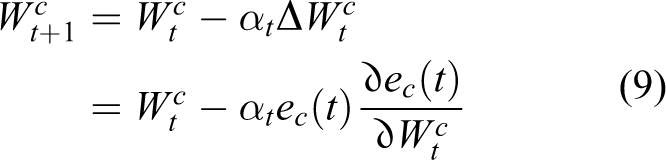
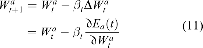
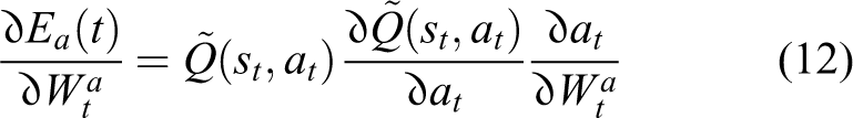
where α_t and β_t are learning rates for the critic and actor networks. Partial derivatives at the right side of equations (10) and (12) can be solved according to the definitions of the networks.

Up to the present, the MDP definition of acceleration decision for the autonomous following problem has been developed. Weight updating rules have been derived for the actor and critic networks of the NDP algorithm. With these preparations, the training process of the two networks can be started. Action value function Q(s, a) and action policy π(s, a) for the acceleration decision problem will be approximated and improved gradually.

Acceleration tracking

Acceleration tracking is the consequent phase after the acceleration decision, which realizes the determined acceleration for the follower vehicle with proper control of throttle and brake. In this article, we assume that the transmission keeps unchanged all along. The acceleration tracking is implemented with an internal model control (IMC) structure, which is proposed for the speed tracking control of autonomous land vehicles in our previous work.³⁹ In this section, IMC structure and the design of our acceleration tracking controller are introduced in detail.

The IMC method relies on the internal model principle which indicates that accurate control can be achieved only if the control systems encapsulate some representation of the plant to be controlled.⁵³ Thus, IMC is a model-based method, and the basic structure is illustrated in Figure 5. The control command u is derived by the controller, which is always the inverse model of the plant to be controlled. Meanwhile, a forward model of the plant is utilized to identify the noise introduced into the system by either internal or external sources. The difference between outputs of the actual plant and the forward model is fed back to the reference as an input to the controller.

Figure 5.

Basic IMC structure. IMC: internal model control,

In our problem, the control reference is the follower’s acceleration. If we assumed that the mass of the vehicle is unchanged, then the acceleration equivalent to tractive force and the feedback acceleration deviation can be directly compensated to the reference acceleration. Thus, the IMC structure is suitable for the acceleration tracking problem. The IMC structure for acceleration tracking is illustrated in the blue dashed block in Figure 2.

The longitudinal system of land vehicles is composed of the engine, transmission, tires, and so on.⁵⁴ Due to the strong nonlinear and obvious delay characteristic, it is difficult to found the mechanistic model. Thus, a nonparametric longitudinal dynamic model is utilized in the IMC acceleration tracking structure. According to the intuitive experience that certain throttle or brake applied to the vehicle at different vehicle speeds will obtain different accelerations, we regard the longitudinal system as a black box and formulate the relationship between the current speed v_c , current control input u, and the next acceleration a as

a = F (v_{c}, u)

To measure the vehicle’s response to different control inputs and establish the nonparametric model,¹³ off-line experiments are taken in the reference environment with flat, straight, and level roads. Details about collecting the longitudinal response data of the vehicle can be found in the study by Wang et al.³⁹

Simulations and discussions

To validate the performance of the proposed method, experiments are carried out on our simulation platform, which is constructed based on the high-fidelity vehicle dynamic simulator, CarSim. As a well-recognized tool in the automotive industry, CarSim can deliver accurate, detailed, and efficient methods for simulating the performance of passenger vehicles.⁵⁵ Our longitudinal controller is implemented with MATLAB and exchanges data with the vehicle simulation solver by the provided API.⁵⁶

Before the learning process starts, structures of the actor and critic networks should be defined clearly. In this article, both actor and critic adopt feedforward neural networks with three layers. Ten neural nodes are set to the hidden layers for the two networks. Activation functions of hidden and output nodes in the actor network are with sigmoid type. Hidden nodes of the critic network are also set as the sigmoid-type activation function. While activation functions of the output nodes in the critic network are with linear type. Both the learning rates α_t and β_t for the two networks are set as 0.01. Discount factor γ which balances the immediate and long-term rewards is set as 0.9. All weight parameters are initialized randomly before training begins.

Since vehicle speed and following distance are continuous, there are infinite initial states with different follower’s speed, leader speed, and initial following distance. Thus, in each learning episode, the initial state is determined by randomly setting the follower’s speed, leader’s speed, and initial following distance. The target following distance for each episode is also confirmed randomly.

After the iterative training procedure, a near-optimal acceleration decision policy is derived. Near-optimal follower’s acceleration actions for a different following state under the learned policy are illustrated in Figure 6. To verify the performance of learned acceleration decision policy, tests are conducted with three representative scenarios. Meanwhile, the smooth trapezoidal curve–based approach (noted as the trapezoidal method below) presented in the study by Li et al.³¹ is also tested in the same scenarios for comparing.

Figure 6.

Follower’s acceleration actions for different states under the learned policy.

Firstly, it is a challenging test (noted as test A), in which the follower’s initial speed is zero and leader’s initial speed is 54 km/h constantly. Initial following distance is 30 m and the target value is 15 m. Since the initial speed of the follower is far less than the leader, and the target follow space is also less than the initial value, the follower vehicle should speed up quickly to catch up to the leader. Regulating process and following results of test A are described in Figure 7.

Figure 7.

The regulating process and following result of test A. Top: leader’s and follower’s speed. Bottom: actual and target following distance.

The upper sub-figure of Figure 7 shows the speed regulation process in test A. The corresponding relations between curves and variables are indicated by the legends in the figures. Both follower’s speeds regulated by our method and trapezoidal method are increased rapidly. Follower’s speed by our method converges to the leader after about 35 s, which is slower than the trapezoidal method (about 20 s). Similar phenomenon and converging time can be found in the lower sub-figure, which describes the regulation process of the following distance.

Follower’s acceleration commands generated by the two compared methods are shown in the left sub-figure of Figure 8. It can be found that the acceleration commands derived by the proposed method are obviously smoother than outputted by the trapezoidal method. Smooth desired acceleration is important to the comfort and safety of vehicle driving. The right sub-figure displays the actual normalized throttle and brake control value exported from CarSim. For convenience, the brake states are multiplied by −1 and shown as negative values. As the dotted blue curve records, sudden brake and throttle are taken by the trapezoidal method. This is uncomfortable and dangerous during driving on the road, especially with high running speed. In contrast, the control states of throttle and brake by our method are milder and more acceptable.

Figure 8.

The acceleration commands and control states of the follower vehicle in test A. Left: decided acceleration and actual acceleration. Right: actual throttle and brake exported from CarSim.

In the second test (noted as test B), the initial speed of the follower is 54 km/h. Leader’s speed is 25 km/h constantly. Initial following distance is 25 m and the target value is set as15 m. Since the follower’s initial speed is obviously larger than the leader, a strong speed reduction should be applied at the very start. Regulating process and following results of test B are described in Figure 9.

Figure 9.

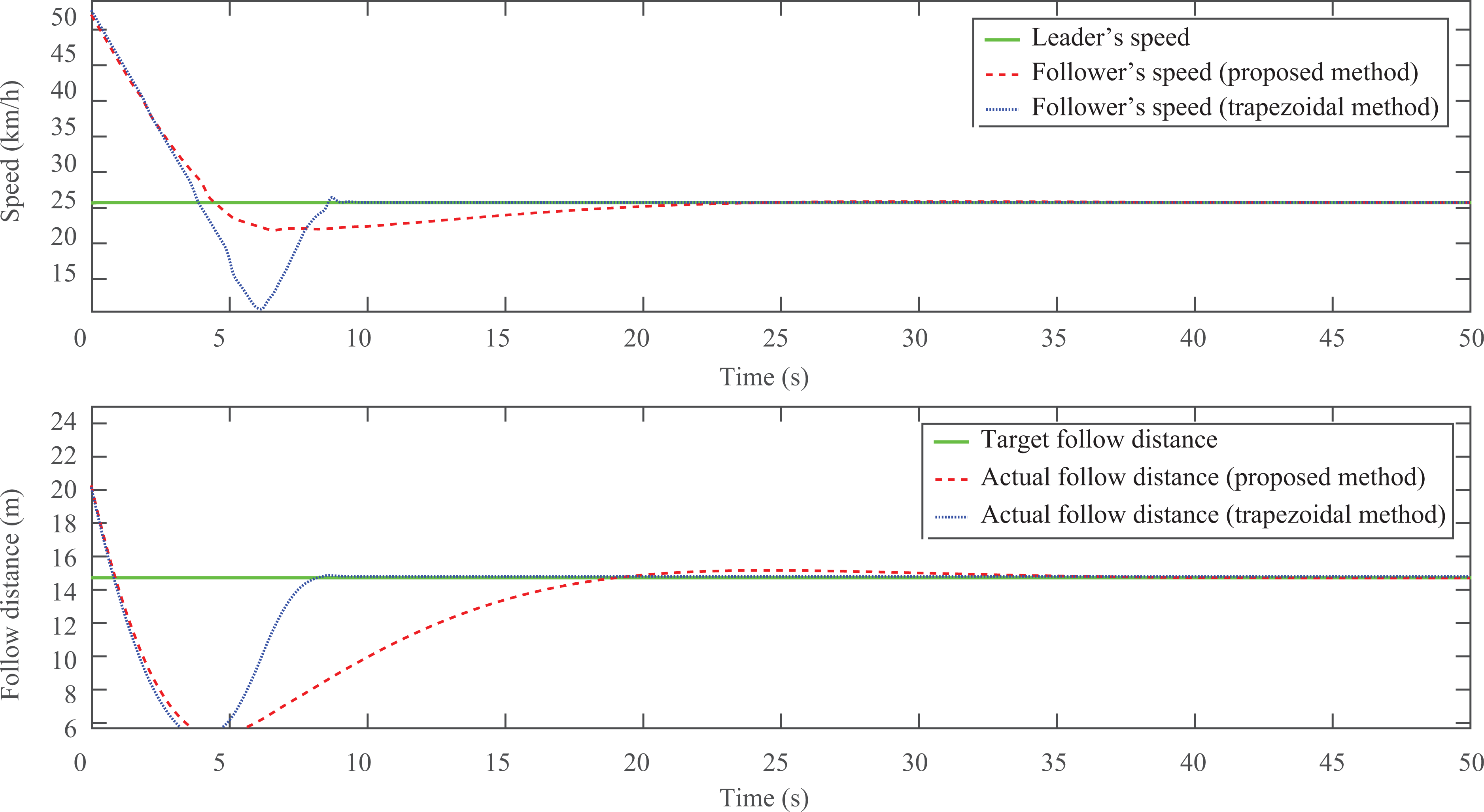
The regulating process and following result of test B. Top: leader’s and follower’s speed. Bottom: actual and target following distance.

From the speed curves described in the upper sub-figure of Figure 9, both the follower’s speeds regulated by the two compared methods are decreased as quickly as expected. Follower’s speed and following distance controlled by the trapezoidal method converge to the leader and target space value at about 10 s, which is far faster than the proposed method (about 30 s). The cost of the fast convergence with the trapezoidal method is the violent driving behavior. This is displayed in Figure 10, which records the desired accelerations and actual throttle/brake states.

Figure 10.

The acceleration commands and control states of the follower vehicle in test B. Left: decided acceleration and actual acceleration. Right: actual throttle and brake exported from CarSim.

Finally is a comprehensive test (noted as test C), in which initial speeds of the follower and leader are zero and 20 km/h. Initial following distance is 35 m and the target value is set as 25 m. Unlike the above two tests, leader’s speed changes with the running time during test C. The acceleration policy should deal with this additional disturbance. Regulating process and following results of test C are described in Figure 11.

Figure 11.

The regulating process and following result of test C. Top: leader’s and follower’s speed. Bottom: actual and target following distance.

Leader’s speed is a timely changed curve as the green solid curve in the upper sub-figure of Figure 11. In the first 100 s, leader’s speed is 20 km/h, then it increases to 50 km/h for the next 100 s. In the third 100 s, it goes back to 30 km/h. Finally, it rises up to 55 km/h. From Figure 11, for both methods, the follower’s speed tracks the changing leader’s speed with small overshoots at every transition position. Following distance converges to the target value after a short regulation at the beginning of every 100 s. Figure 12 shows the acceleration commands and the control states of follower vehicle in test C.

Figure 12.

The acceleration commands and control states of the follower vehicle in test C. Left: decided acceleration and actual acceleration. Right: actual throttle and brake exported from CarSim.

Comparing with the two tested methods, regulation process of the trapezoidal method is more decisive, while the proposed learning-based method is smoother. This difference is reflected obviously in the desired acceleration results as the left sub-figures of Figures 8, 10, and 12, in which the magnitudes and regulation of the desired acceleration commands derived from the trapezoidal method are larger than the proposed method. With the drastic acceleration action, the trapezoidal method can regulate to the steady state more quickly. But, this kind of behavior may lead to the ride comfortlessness and unsafety during the following process. On the other hand, desired acceleration commands of our method in this article are smoother and more human-like. This advantage is mainly achieved by the punishment component on the changing of the acceleration actions in the reward function as in equation (6). Consequently, the proposed method needs more regulating time and small overshoots exist due to the mild acceleration behavior. This is acceptable considering the safety and smoothness. From the tests above, the performance of the presented longitudinal control approach for the autonomous following problem is well demonstrated. Compared to the trapezoidal method, our approach can ensure the smoothness, comfort, and safety during the autonomous follow driving process.

Conclusions and future work

The autonomous follow driving problem of two-vehicle platoon is investigated in this article. The longitudinal control of the follower vehicle is divided into two phases: acceleration decision and acceleration tracking. NDP, an actor–critic RL algorithm, is utilized to learn a near-optimal acceleration decision policy through iteratively trial and error. An IMC structure is designed to adaptively control the follower vehicle as the decided acceleration. Acceleration decision policy learning and performance verification tests are conducted with CarSim. From the test results, it can be found that the proposed method is competent for the autonomous following problem.

For the proposed method, there are small overshoots during the following distance regulation process, especially when large deviations from the initial state and target state exist. This is partly because of the near-optimal property of the NDP algorithm. Thus, more intelligent learning approach will be employed in the future. And more ingenious reward functions of the autonomous following MDP should be designed to deal with these shortcomings and further improve the performance. Besides, the longitudinal regulation method in this article will be combined with proper lateral controllers to construct a complete autonomous following system. And more experiments will be conducted on real vehicles to verify the performance of the proposed longitudinal control approach.

Footnotes

Acknowledgements

The authors would like to thank the anonymous reviewers for their valuable comments.

Declaration of conflicting interests

The author(s) declared no potential conflicts of interest with respect to the research, authorship, and/or publication of this article.

Funding

The author(s) disclosed receipt of the following financial support for the research, authorship, and/or publication of this article: The work is supported by National Nature Science Foundation of China under grant no. 61375050.

References

Thrun

Montemerlo

Dahlkamp

. Stanley: the robot that won the DARPA Grand Challenge. J Field Robot 2006; 23(9): 1–43.

Urmson

Anhalt

Bagnell

. Autonomous driving in urban environments: Boss and the Urban Challenge. J Field Robot 2008; 25(8): 425–466.

Montemerlo

Becker

Bhat

. Junior: the Stanford entry in the urban challenge. J Field Robot 2008; 25(9): 569–597.

Mirzabeiki

. An overview of freight intelligent transportation systems. Int J Logist Syst Manage 2013; 14(4): 473–489.

Guo

Luo

. Adaptive coordinated leader-follower control of autonomous over-actuated electric vehicles. Transactions of the Institute of Measurement and Control 2016; doi: 10.1177/0142331216648374.

Caudill

Garrard

. Vehicle-follower, longitudinal control for automated transit vehicles. IEEE Trans Veh Technol 1977; 28(1): 36–45.

Swaroop

Rajagopal

. A review of constant time headway policy for automatic vehicle following. In: Proceedings of IEEE Intelligent Transportation Systems, Oakland, CA, USA, 25–29 August 2001, pp. 65–69.

Ioannou

. Throttle and brake control systems for automatic vehicle following. J Int Trans Syst 1994; 1(4): 345–377.

Lygeros

Godbole

DN,

Sastry

. Verified hybrid controllers for automated vehicles. IEEE Trans Autom Control 1998; 43(4): 522–539.

10.

Guvenc

Kural

. Adaptive cruise control simulator: a low-cost, multiple-driver-in-the-loop simulator. IEEE Control Syst 2006; 26(3): 42–55.

11.

Guzman

Adams

. Autonomous vehicle-following systems: a virtual trailer link model. In: IEEE/RSJ International Conference on Intelligent Robots and Systems, Edmonton, Alta., Canada, 2–6 August 2005, pp. 3057–3062.

12.

. Autonomous vehicle following system—a virtual trailer link approach. PhD Thesis, Nanyang Technological University, Singapore, 2009.

13.

Chen

Zhang

. Vehicle following algorithm realization based on a virtual flexible curved bar with force delay. In: IEEE International Conference on Robotics and Automation, Shanghai, China, 9–13 May 2011, pp. 90–95.

14.

Wang

. An autonomous vehicle following approach—the virtual flexible bar model. In: IEEE Conference Anthology, China, 1–8 January 2013, pp. 1–6.

15.

Hedrick

Drew

. Acc/cacc-control design, stability and robust performance. In: Proceedings of the American Control Conference, Anchorage, AK, USA, 8–12 May 2002, pp. 4327–4332.

16.

Mullakkal-Babu

Wang

van Arem

. Design and analysis of full range adaptive cruise control with integrated collision a voidance strategy. In: IEEE 19th International Conference on Intelligent Transportation Systems (ITSC), Rio de Janeiro, Brazil, 1–4 November 2016, pp. 308–315.

17.

Muller

Nocker

. Intelligent cruise control with fuzzy logic. In: Proceedings of the Intelligent Vehicles Symposium, Detroit, MI, USA, 29 June–1 July 1992, pp. 173–178.

18.

Chang

Choi

. Automatic vehicle following using the fuzzy logic. In: Proceedings of Vehicle Navigation and Information Systems Conference, Seattle, WA, USA, 30 July–2 August 1995, pp. 206–213.

19.

Fritz

Schiehlen

. Nonlinear ACC in simulation and measurement. Vehicle Syst Dyn 2001; 36(2–3): 159–177.

20.

Xiao

Gao

. Practical string stability of platoon of adaptive cruise control vehicles. IEEE Trans Intell Transp Syst 2011; 12(4): 1184–1194.

21.

Ghaffari

Gharehpapagh

Khodayari

. Longitudinal and lateral movement control of car following maneuver using fuzzy sliding mode control. In: IEEE 23rd International Symposium on Industrial Electronics (ISIE), Istanbul, Turkey, 1–4 June 2014, pp. 150–155.

22.

Moon

. Design, tuning, and evaluation of a full-range adaptive cruise control system with collision avoidance. Control Eng Pract 2009; 17(4): 442–455.

23.

Kim

Lee

Kim

. Integrated risk management based automated vehicle following system on inner-city streets. In: 17th International IEEE Conference on Intelligent Transportation Systems (ITSC), Qingdao, China, 8–11 October 2014, pp. 418–423.

24.

Kim

. Design of a model reference cruise control algorithm. SAE Int J Passeng Cars 2012; 5(2): 440–449.

25.

Guillet

Lenain

Thuilot

. Adaptable robot formation control: adaptive and predictive formation control of autonomous vehicles. IEEE Robot Autom Mag 2014; 21(1): 28–39.

26.

Bom

Thuilot

Marmoiton

. A global control strategy for urban vehicles platooning relying on nonlinear decoupling laws. In: IEEE/RSJ International Conference on Intelligent Robots and Systems, Edmonton, Alta., Canada, 2–6 August 2005, pp. 2875–2880.

27.

Stanger

del Re

. A model predictive cooperative adaptive cruise control approach. In: American Control Conference, Washington, DC, USA, 17–19 June 2013, pp. 1374–1379.

28.

Shakouri

Ordys

. Nonlinear model predictive control approach in design of adaptive cruise control with automated switching to cruise control. Control Eng Pract 2014; 26(1): 160–177.

29.

Moser

Waschl

Kirchsteiger

. Cooperative adaptive cruise control applying stochastic linear model predictive control strategies. In: European Control Conference (ECC), Linz, Austria, 15–17 July 2015, pp. 3383–3388.

30.

Kayacan

. Multiobjective h_∞ control for string stability of cooperative adaptive cruise control systems. IEEE Trans Intell Veh 2017; 2(1): 52–61.

31.

Sun

Cao

. Real-time trajectory planning for autonomous urban driving: framework, algorithms, and verifications. IEEE/ASME Trans Mechatron 2016; 21(2): 740–753.

32.

Sutton

Barto

. Reinforcement learning: an introduction. IEEE Trans Neural Netw 1998; 9(5): 1054.

33.

Liu

. Continuous-action reinforcement learning with fast policy search and adaptive basis function selection. Soft Comput 2010; 15(6): 1055–1070.

34.

Pardalos

. Approximate dynamic programming: solving the curses of dimensionality. Optim Methods Softw 2009; 24(1): 155.

35.

Wiering

Otterlo

. Reinforcement learning: state-of-the-art. Phillip J Fr Restaur Zahnmed 2012; 20(2): 57.

36.

Desjardins

Chaib-Draa

. Cooperative adaptive cruise control: a reinforcement learning approach. IEEE Trans Intell Transp Syst 2006; 12(4): 1248–1260.

37.

Zhao

Xia

. Full-range adaptive cruise control based on supervised adaptive dynamic programming. Neurocomputing 2014; 125: 57–67.

38.

Zhu

Huang

Liu

. An adaptive path tracking method for autonomous land vehicle based on neural dynamic programming. In: 2016 IEEE International Conference on Mechatronics and Automation, Harbin, China, 7–10 August 2016, pp. 1429–1434.

39.

Wang

Sun

. Adaptive speed tracking control for autonomous land vehicles in all-terrain navigation: an experimental study. J Field Robot 2013; 30(1): 102–128.

40.

Liu

Sun

. Weakly paired multimodal fusion for object recognition. IEEE Trans Autom Sci Eng 2017; PP(99): 1–12.

41.

Liu

Sun

. Visual-tactile fusion for object recognition. IEEE Trans Autom Sci Eng 2017; 14(2): 996–1008.

42.

Chen

Wang

Dai

. Likelihood-field-model-based dynamic vehicle detection and tracking for self-driving. IEEE Trans Intell Transp Syst 2016; 17(11): 3142–3158.

43.

Chen

Dai

Liu

. Likelihood-field-model-based vehicle pose estimation with velodyne. In: IEEE 18th International Conference on Intelligent Transportation Systems, Las Palmas, Spain, 15–18 September 2015, pp. 296–302.

44.

Liu

Sun

Fang

. Robotic room-level localization using multiple sets of sonar measurements. IEEE Trans Instrum Meas 2016; PP(99): 1–12.

45.

Jia

Ngoduy

. Platoon based cooperative driving model with consideration of realistic inter-vehicle communication. Trans Res C Emerg Technol 2016; 68: 245–264.

46.

Sun

Huang

Zhu

. High-precision motion control method and practice for autonomous driving in complex off-road environments. In: IEEE Intelligent Vehicles Symposium (IV), Gothenburg, Sweden, 19–22 June 2016, pp. 767–773.

47.

Wang

. Online learning control by association and reinforcement. IEEE Trans Neural Netw 2001; 12(2): 264–276.

48.

Sutton

Barto

. Reinforcement Learning: An Introduction. Cambridge, USA: MIT Press, 1998.

49.

Bertsekas

. Dynamic Programming and Optimal Control. Cambridge, USA: Athena Scientific, Massachusetts Institute of Technology, 2000.

50.

Bellman

. Dynamic Programming. Princeton, USA: Princeton University Press, 1957.

51.

Howard

. Dynamic programming and Markov processes. Cambridge, USA: MIT Press, 1960.

52.

Busoniu

Ernst

Schutter

. Approximate reinforcement learning: An overview. In: IEEE Symposium on Adaptive Dynamic Programming and Reinforcement Learning (ADPRL), Paris, France, 11–15 April 2011, pp. 1–8.

53.

Francis

Wonham

. The internal model principle of control theory. Automatica 1976; 12(5): 457–465.

54.

Rajamani

. Vehicle dynamics and control. US: Springer, 2006.

55.

Snider

. Automatic steering methods for autonomous automobile path tracking. Pittsburgh, PA: Technical Report CMU-RI-TR-09-08, Robotics Institute, Carnegie Mellon University, 2009.

56.

Sun

Zhu

. A unified approach to local trajectory planning and control for autonomous driving along a reference path. In: IEEE International Conference on Mechatronics and Automation, Tianjin, China, 3–6 August 2014, pp. 1716–1721.

An adaptive longitudinal control method for autonomous follow driving based on neural dynamic programming and internal model structure

Abstract

Keywords

Introduction

Overall

Acceleration decision based on NDP

Markov decision process

Modeling the acceleration decision problem with MDP

Learning the acceleration policy with NDP

Acceleration tracking

Simulations and discussions

Conclusions and future work

Footnotes

Acknowledgements

Declaration of conflicting interests

Funding

References