Sage Journals: Discover world-class research

Abstract

Robot manipulators are mostly used to complete positioning tasks, and the conventional approach utilizes position-based control scheme, which converts a robot control problems to several motor control problems, where encoder signals are used to fulfill feedback control. This control scheme might not provide excellent positioning accuracy due to the lack of the dynamics of robot manipulators. This article presents a simple model-based control scheme to achieve the positioning control and applies the scheme to a Delta robot, which can perform the motion with three translational degrees of freedom. The proposed scheme first evaluates the applied torques of motors based on robot’s kinematics and dynamics using the encoders, and then the evaluated torques are sent to controllers to fulfill feedback control. The entire control loop is little similar to torque control, but torque or current sensors are not used. To demonstrate the performances of the proposed scheme, not only the numerical simulations are performed but also the experimental work is conducted. Both results are compared with those by applying the position-based control. The results show that the proposed model-based control scheme provides better positioning accuracy.

Keywords

Delta robot motion control model-based control

Introduction

Parallel robot manipulators have broadly applied in industry due to their advantages such as high speed, high stiffness, high accuracy, low moving inertia, and so on. The Delta robot is one of the most common parallel robot manipulators, because it is usually applied to operate a pick-and-place task under the requirements of high moving speed and high positioning accuracy.^1,2

Over the past decades, there are numerous researchers studied the motion control of a Delta robot. Castañeda et al. designed an adaptive controller, which aims to achieve the trajectory tracking for a Delta robot with uncertainties. Besides, the adaptive controller is incorporated with an observer due to the lack of the measurements of the joint velocities of the Delta robot.³ Ramírez-Neria et al. investigated a robust trajectory tracking, where the controller is based on a linear feedback control and is capable of actively rejecting disturbance using a linear disturbance observer.⁴ Guglielmetti and Longchamp developed a Delta robot model, where the state variables are the joint angles and the end-effector coordinates. Besides, the applied torques can be evaluated for the purpose of achieving a linear feedback control.⁵ Lu et al. developed a type-2 fuzzy logic controller for the trajectory tracking control of the Delta robot. The controller is designed based on a type-1 fuzzy logic controller, whose membership functions are blurred by three methods to generate the type-2 fuzzy sets.⁶ Dumlu and Erenturk applied the classical proportional-integral-derivative (PID) control and the fractional-order PID control to a Delta robot so as to improve the trajectory tracking performances. The controller parameters are obtained using the pattern search algorithm and mathematical methods for the classical PID control and the fractional-order PID controller, respectively.⁷ Lin et al. implemented a smoothing robust control method, manifold deformation design scheme, to guarantee the smoothly and robustly dynamic behavior as designed.⁸ This method has the capabilities of dynamics prediction and disturbance estimation and then outputs the control efforts to deform the dynamic manifold of the controlled plant into the desired manifold. Zhang et al. investigated the conveyor tracking of a Delta robot, and the controller design is based on a computer vision system and encoder signals so as to compute the joint torques.⁹ Rachedi et al. applied the H^∞ controller to a Delta robot, where the controller is multi-input multi-output centralized feedforward control based on the computed joint torques.¹⁰

Generally speaking, there are two types of control schemes for robot manipulators, position- and model-based control. The position-based control divides a manipulator as many separated active joint systems, and each active joint is considered as position control of a motor.^{11
–13} This type of control scheme might not always produce high positioning accuracy due to the lack of the dynamics of manipulators. However, the model-based control incorporates the dynamics in the controllers. Many researchers studied various model-based controls and applied them to robot manipulators. Diaz-Rodriguez et al. applied a passivity-based controller to a three degrees of freedom (3-DOFs) prismatic-revolute-spherical parallel manipulator, where a manipulator is simplified as a reduced model.¹⁴ Zhang et al. proposed an ankle assessment and rehabilitation robot, which can perform a real-time ankle-assessment three-dimensional (3-D) robotic training, where the control is an open-loop controller.¹⁵ Besides, an experiment was performed on a healthy person. Meng et al. investigated a trajectory tracking of a 6-DOF parallel robot, where a model-based controller was proposed based on the off-line multibody dynamics of the robot. This approach can save the online computations.¹⁶ Gao et al. proposed a three-axis parallel mechanism, which is used to test the reliability of multiaxis CNC machine tools. The mechanism exerts specific load spectrums on the spindle, and the dynamic model is derived by employing the virtual work principle. Besides, the controller is designed based on the established model.¹⁷ Zhang et al. developed a trajectory tracking controller and applied it to a 2-DOF translational parallel manipulator, which is driven by linear motors.¹⁸ The controller is designed based on a dynamic model, where a cascade PID/PI controller and a velocity feedforward controller are incorporated.

To obtain precise position control without implementing additional sensors, the computed torque control is developed based on inverse dynamics of robots. Codourey presented the control of a Delta robot by implementing the computed torque approach, where the torque is obtained by applying the dynamic equations, which is derived based on the virtual work principle.^19,20 The derived equations lead to complicated formulations, because the mass matrix in the equations is determined using the Jacobian matrices for each component in the robot. Therefore, the author proposed an approach to simplify the mass matrix, which does not explicitly appear in the formulations. Yang et al. investigated the motor-mechanism dynamics of a 2-DOF parallel manipulator, and the computed torque control combined with a PID controller was applied to the manipulator, where the controller parameters are determined using the three-layer neural network algorithm based on the errors of the angular displacements and velocities.²¹ Conventionally, the computed torque control is usually applied with a linear PD controller. Shang and Cong developed a nonlinear computed torque control to combine with a nonlinear PD controller and applied the control to a planar parallel manipulator, whose stability is proven using the Lyapunov theorem.²² Shang et al. proposed an adaptive computed torque controller for the trajectory tracking of a 2-DOF parallel manipulator with redundant actuation, and the dynamic model includes the frictions of active joints, which are determined by the adaptive laws.²³ Masarati applied it to redundant manipulators using general-purpose multibody formulations and software tools, where the control scheme consists of inverse kinematics to compute positions, velocities, and accelerations and inverse dynamics problem to compute feedforward generalized driving forces.²⁴

In reviewing literature, the computed torque control relies on inverse dynamics combined with a tracking control of angular displacements and velocities, and some researchers applied the control law with feedforward control. This article aims to provide a simple model-based control scheme, where the computed torques are obtained based on kinematics and dynamics of manipulators without applying feedforward control. The control scheme is little similar to a torque control, but torque or current sensor is not implemented. Thus, encoders are the only sensors used to compute the applied torques. The proposed approach is applied to a Delta robot, whose motion has three translating DOFs. This article is organized as follows. “Kinematics and dynamics of a Delta robot” section introduces the kinematics and the dynamics of the Delta robot. “Model-based tracking control” section proposes a model-based control scheme for the robot. “Experimental setup” section presents the experimental setup and validation. “Experimental and simulation results” section demonstrates the experimental and simulation results. “Conclusions” section summarizes some significant conclusions.

Kinematics and dynamics of a Delta robot

A Delta robot consists of three kinematic chains, and each chain consists of two links (A_iB_i and B_iD_i, where i = 1, 2, 3, see Figure 1). Each chain links a fixed base (triangle A₁A₂A₃) and a moving platform (or called an end effector, triangle D₁D₂D₃), where three motors are mounted at points A_i to drive links A_iB_i. A coordinate system is defined on the fixed base, and the origin is located at its center, where the X-axis is arbitrarily defined on the base, the Z-axis is downward and perpendicular to the base, and the Y-axis is orthogonal to the X- and Z-axes. Thus, the motion of the end effector is driven by the three motors through the three kinematic chains, and the end effector has the 3-DOF translating motions. Based on the geometry of the Delta robot, each point A_i has 1-DOF rotating motions, and each points B_i and D_i have 2-DOF rotating motions.

Figure 1.

Schematic diagram of a Delta robot.

Kinematics

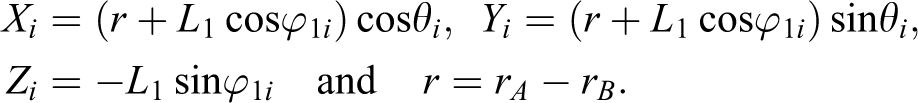
The size of each kinematic chain is assumed to be identical as shown in Figure 2, where L₁, L₂, r_A, and r_B are the lengths of B_iD_i, A_iB_i, OA_i, and D_iP, respectively; φ_1i is the rotating angle of link A_iB_i with respect to the fixed base; φ_2i and φ_3i are the rotating angles of link B_iD_i with respect to link A_iB_i. Based on the geometry of the Delta robot, the position of point P at end effector with respect to the XYZ coordinate is written as

Figure 2.

Schematic diagram of a kinematic chain (a) from a 3-D view and (b) on the x–y plane.

[\begin{matrix} X_{P} \\ Y_{P} \\ Z_{P} \end{matrix}] = [\begin{matrix} cos θ_{i} (r_{A} - r_{B} + L_{1} cos ϕ_{1 i} + L_{2} cos (ϕ_{1 i} + ϕ_{2 i}) cos ϕ_{3 i}) - L_{2} sin θ_{i} sin ϕ_{3 i} \\ sin θ_{i} (r_{A} - r_{B} + L_{1} cos ϕ_{1 i} + L_{2} cos (ϕ_{1 i} + ϕ_{2 i}) cos ϕ_{3 i}) + L_{2} sin θ_{i} cos ϕ_{3 i} \\ L_{1} sin ϕ_{1 i} + L_{2} sin (ϕ_{1 i} + ϕ_{2 i}) cos ϕ_{3 i}) \end{matrix}], (i = 1, 2, 3)

Equation (1) represents the position of point P through one of the three kinematic chains. By eliminating the passive joint angles ϕ_2i and ϕ_3i, equation (1) can be simplified as

{(X_{P} - X_{i})}^{2} + {(Y_{P} - Y_{i})}^{2} + {(Z_{P} - Z_{i})}^{2} = L_{2}^{2}, (i = 1, 2, 3)

where

X_{i} = (r + L_{1} cos ϕ_{1 i}) cos θ_{i}, Y_{i} = (r + L_{1} cos ϕ_{1 i}) sin θ_{i}, Z_{i} = - L_{1} sin ϕ_{1 i} and r = r_{A} - r_{B} .

Direct kinematics

The direct kinematics determines the position (X_P,Y_P,Z_P) of the end effector of a Delta robot using the given active joint angles ϕ_1i. Equation (1) represents three spherical equations, whose center and radius are (X_i, Y_i, Z_i) and L₂, respectively, and the equations are functions of the position (X_P,Y_P,Z_P). Therefore, the intersection of the three spheres is the solution of equation (1). Besides, there are four possibilities after solving the equations (for more details see the study by Tsai²⁵).

Inverse kinematics

The indirect kinematics determines the active joint angles ϕ_1i based on a given position (X_P,Y_P,Z_P) of the end effector. By expanding equation (2), the equation can be reduced as

l_{i} cos ϕ_{1 i} + m_{i} sin ϕ_{1 i} = n_{i}, (i = 1, 2, 3)

where

l_{i} = 2 r L_{1} - 2 L_{1} X_{P} cos θ_{i} - 2 L_{1} Y_{P} sin θ_{i}, m_{i} = 2 L_{1} Z_{P}, and n_{i} = 2 r X_{P} cos θ_{i} - 2 r Y_{P} sin θ_{i} + X_{P}^{2} + Y_{P}^{2} + Z_{P}^{2} + L_{1}^{2} - L_{2}^{2} + r^{2}

Equation (3) refers to the functions of the active angles ϕ_1i, which can be determined by a single equation of equation (3), and four possibilities can be obtained after solving the equation.²⁶

Workspace

The workspace of the Delta robot is a 3-D region which can be attained by the end effector of the robot. Based on equation (3) and trigonometry, the equation must satisfy the condition as

| \frac{n_{i}}{\sqrt{l_{i}^{2} + m_{i}^{2}}} | \leq 1

Note that equation (5) is a function of the position (X_P,Y_P,Z_P) of the end effector only. Therefore, substituting any position (X_P,Y_P,Z_P) can check if it is within the workspace of the robot or not.

Singularities

The singularities of the Delta robot interpret the relationships between the joint rates of the Delta robot and the velocities of the end effector. There are two types of singularities, direct singularities and inverse singularities, and they are determined by examining the singularities of Jacobian matrices. Taking the time derivative of equation (2) leads to

J_{P} \overset{⇀}{v} = J_{φ} \dot{\overset{⇀}{φ}}

where

\begin{array}{l} \overset{⇀}{v} = {[\begin{matrix} {\dot{X}}_{p} & {\dot{Y}}_{p} & {\dot{Z}}_{p} \end{matrix}]}^{T}, \dot{\overset{⇀}{ϕ}} = {[\begin{matrix} {\dot{ϕ}}_{1 i} & {\dot{ϕ}}_{2 i} & {\dot{ϕ}}_{3 i} \end{matrix}]}^{T}, J_{P} = [\begin{matrix} J_{1 x} & J_{1 y} & J_{1 z} \\ J_{2 x} & J_{2 y} & J_{2 z} \\ J_{3 x} & J_{3 y} & J_{3 z} \end{matrix}], J_{i x} = sin ϕ_{3 i} cos (ϕ_{1 i} + ϕ_{2 i}) cos θ_{i} + cos ϕ_{3 i} sin θ_{i}, \\ J_{i y} = - sin ϕ_{3 i} cos (ϕ_{1 i} + ϕ_{2 i}) cos θ_{i} + cos ϕ_{3 i} cos θ_{i}, J_{i z} = sin ϕ_{3 i} sin (ϕ_{1 i} + ϕ_{2 i}), and \\ J_{ϕ} = diag (sin ϕ_{21} sin ϕ_{31}, sin ϕ_{22} sin ϕ_{32}, sin ϕ_{23} sin ϕ_{33}) . \end{array}

The direct singularities are determined by calculating the roots of the determinant of J_P. Although it is complicated to find them, a solutions is ϕ_3i = 0, π or ϕ_1i + ϕ_2i = 0, π.¹⁷ Similarly, the inverse singularities are determined by evaluating the roots of the determinant of J_ϕ, and the solutions are ϕ_2i = 0, π or ϕ_3i = 0, π.

Dynamics

To investigate the dynamics of the robot, one assumes that there are no frictions on all joints and no flexibility on all links. The dynamic equations of the robot will be formulated by applying the Lagrange’s equations. The kinetic and potential energies of the robot are first written as

T_{m} = \frac{1}{2} m_{P} ({\dot{X}}_{P}^{2} + {\dot{Y}}_{P}^{2} + {\dot{Z}}_{P}^{2}) + \frac{1}{6} m_{1} L_{1}^{2} \sum_{i} {\dot{φ}}_{1 i}^{2} + \frac{1}{2} m_{2} \sum_{i} ({\dot{X}}_{P}^{2} + {\dot{Y}}_{P}^{2} + {\dot{Z}}_{P}^{2} + L_{1}^{2} {\dot{φ}}_{1 i}^{2})

V_{m} = m_{P} g Z_{P} + \frac{1}{2} m_{1} g L_{1} \sum_{i} sin φ_{1 i} + m_{2} g \sum_{i} (Z_{P} + L_{1} sin φ_{1 i})

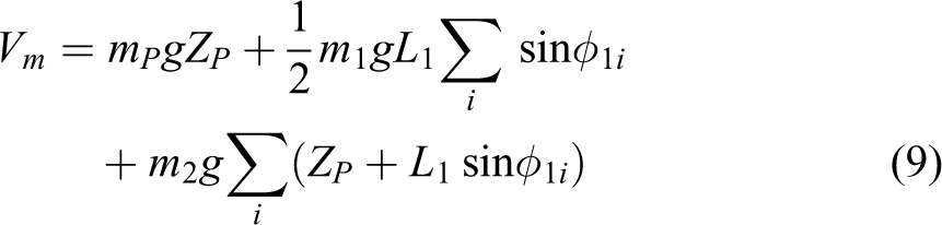
where m_P, m₁, and m₂, respectively, refer to the masses of the end effector, the links A_iB_i, and the links B_iD_i.

Since equations (8) and (9) are the functions of six variables X_P, Y_P, Z_P, and φ_1i, the Lagrangian should incorporate with three constraint equations as equation (2), which leads to the dynamic equations as

(m_{P} + 3 m_{2}) {\ddot{X}}_{P} - 2 \sum_{i} λ_{i} (X_{P} + r cos θ_{i} - L_{1} cos ϕ_{1 i} cos θ_{i}) = F_{P X}

(m_{P} + 3 m_{2}) {\ddot{Y}}_{P} - 2 \sum_{i} λ_{i} (Y_{P} + r sin θ_{i} - L_{1} cos ϕ_{1 i} sin θ_{i}) = F_{P Y}

(m_{P} + 3 m_{2}) {\ddot{Z}}_{P} - 2 \sum_{i} λ_{i} (Z_{P} - L_{1} sin ϕ_{1 i}) + (m_{P} + 3 m_{2}) g = F_{P Z}

\begin{array}{l} (\frac{1}{3} m_{1} + m_{2}) L_{1}^{2} {\ddot{ϕ}}_{1 i} + (\frac{1}{2} m_{1} + m_{2}) g L_{1} cos ϕ_{1 i} \\ - 2 λ_{i} L_{1} [(X_{P} cos θ_{i} + Y_{P} sin θ_{i} + r) sin ϕ_{1 i} - Z_{P} cos ϕ_{1 i}] = τ_{i}, (i = 1, 2, 3) \end{array}

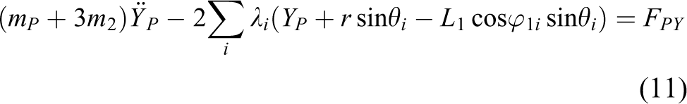
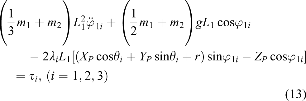
where λ_i are the Lagrange multipliers; F_PX, F_PY, and F_PZ are the applied external forces at the point P; τ_i are the applied external torques at the active joints. Note that equations (10) to (13) are functions of nine variables X_P, Y_P, Z_P, φ_1i, and λ_i. Therefore, the equations will be solved with the constraint equations as equation (2). These equations are differential-algebraic equations.

An alternative application of the equations is used to determine the applied torques τ_i, and the procedure is explained as follows.

The kinematic equations shown in equation (2) are solved, and then the active angles ϕ_1i and the coordinates X_P, Y_P, and Z_P can be obtained. Moreover, the first- and second-time derivatives can be calculated.

The Lagrange multipliers λ_i can be obtained by solving equations (10) to (12), where the applied forces F_PX, F_PY, and F_PZ are given.

The applied torques τ_i can be calculated using equation (13).

This procedure can be used for a torque control of the robot. Besides, the proposed control scheme applies this procedure to compute the desired torques and the real torques, which will be presented in the next section.

Model-based tracking control

Path planning

A Delta robot is usually applied to a pick-to-place operation. For a specific 3-D trajectory such as a straight line, a circle, a parabola, and so on, the path can be expressed as a parametric function q(u), where q refers to coordinates x, y, and z and u is a parameter to define the path from the initial position to the final position. To maintain zero oscillations when the picking and placing operations are performed, one intends to plan a path with zero oscillations at the initial and final positions of the path. Thus, the parameter u can be replaced by a quintic polynomial function of time:

u (t) = a_{0} + a_{1} t + a_{2} t^{2} + a_{3} t^{3} + a_{4} t^{4} + a_{5} t^{5}

with the boundary conditions as $u (t_{0}) = u_{0}$ , $\dot{u} (t_{0}) = 0$ , $\ddot{u} (t_{0}) = 0$ , $u (t_{f}) = u_{f}$ , $\dot{u} (t_{f}) = 0$ , and $\ddot{u} (t_{f}) = 0$ , where u₀ and u_f are two given parameters referring to the initial and final positions, and the coefficients a_i can be determined by these boundary conditions.

By differentiating equation (14) with respect to time, the velocity and acceleration of any point on the path can be, respectively, obtained as

\dot{q} (u) = \dot{u} \frac{d q}{d u}, \ddot{q} (u) = \ddot{u} \frac{d q}{d u} + {\dot{u}}^{2} \frac{d^{2} q}{d u^{2}}

\dot{u} = \dot{q} (u) / \frac{d q}{d u}, \ddot{u} = (\ddot{q} (u) - {\dot{u}}^{2} \frac{d^{2} q}{d u^{2}}) / \frac{d q}{d u}, (\frac{d q}{d u} \neq 0)

Note that equation (16) is used to determine the boundary conditions so as to solve equation (14) for the coefficients a_i.

For the initial and final positions, substituting those boundary conditions into equation (15) leads to zero velocities, $\dot{q} (u_{0})$ and $\dot{q} (u_{f})$ , as well as the accelerations, $\ddot{q} (u_{0})$ and $\ddot{q} (u_{f})$ . Therefore, the results imply that there are no oscillations at both positions by following the aforementioned path planning approach.

Tracking control

Position-based control

The position-based control converts a robot control problem to several motion control problems, and each motor is achieved by the position tracking control. Based on the aforementioned path planning, the desired coordinates of the end effector can be obtained, and then they can be used to determine the desired active joint angles by applying the inverse kinematics. A controller will be designed to achieve the tracking control of the active joint angles, which are generated from the motors mounted on the active joints, and the active joint angles are considered to be measurable using encoders. The active joint angles generated from the motors can be used to determine the coordinates of the end effector by applying the direct kinematics.

Actually, the entire control system is a semi-closed loop system, and only the dynamics of the motors and the kinematics of the Delta robot are included in the system. Figure 3(a) shows the block diagram of the control system, where E_i are the voltages applied to the motors, and the subscript d refers to reference signals. The first block is the path planning, which can generate the desired trajectories of the end effector expressed as the coordinate functions of time, (X_P)_d, (Y_P)_d, and (Z_P)_d. The second block is the inverse kinematics, which can convert the coordinates (X_P)_d, (Y_P)_d, and (Z_P)_d to the desired active joint angles (ϕ_1i)_d. The third block is a controller, which computes voltage signals E_i of the motors based on the desired active joint angles (ϕ_1i)_d and the measured joint angles ϕ_1i. The last block is the direct kinematics, which can evaluates the actual coordinates X_p, Y_p, and Z_p. Note that the third block consists of a motor and a driver for an experimental work, and the block is modeled as a second-order transfer function with a time delay, which is expressed as

Figure 3.

Block diagram of (a) a position-based control and (b) a model-based control.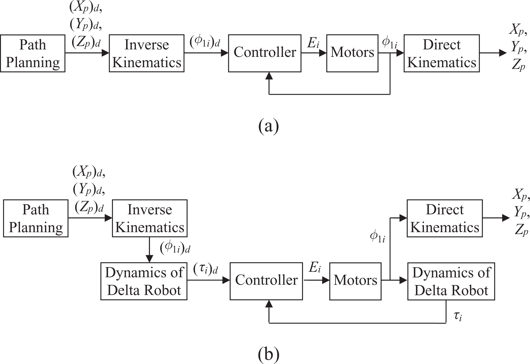

G (s) = \frac{K_{m} e^{- T_{m 2} s}}{s (T_{m 1} s + 1)}

where K_m is a gain, T_m1 is a time constant, and T_m2 is delay time. They are model parameters, which will be determined by applying the system identification to the block.

Model-based control

The aforementioned control system is broadly applied to various industrial robot manipulators. It can be seen that the dynamics of the Delta robot is not included in the control system, so the dynamic characteristics of the robot will not be shown in the system. To keep the simplicity of the entire system without applying any additional sensors and to incorporate the dynamics into the control system, a model-based loop system is proposed as shown in Figure 3(b). To compare it with Figure 3(a), the proposed control system still uses the encoders to obtain the active joint angles, and there are two additional blocks included in the block diagram, which are the dynamics of the Delta robot. The block converts the desired coordinates (X_P)_d, (Y_P)_d, and (Z_P)_d to the desired motor torques (τ_i)_d based on equations (10) to (13). Similarly, the same block converts the actual coordinates X_p, Y_p, and Z_p to the actual motor torques τ_i based on the same equations. It is worth noting that a central difference technique is used to calculate ${\dot{ϕ}}_{1 i}$ and ${\ddot{ϕ}}_{1 i}$ before applying the conversion procedures.

Experimental setup

Experimental delta robot

An experimental Delta robot is designed and is manufactured as shown in Figure 4. The robot is composed of a moving platform, a fixed base, and three kinematic chains. The moving platform is also called the end effector, which is the member connected by three passive links as shown in Figure 4. The fixed base is the top plane, which is used to fix motors. The kinematic chain consists of an upper arm and a lower arm, where the upper arm is a link connected by a motor, and the lower arm has four links, which form four-bar mechanisms as shown in Figure 4. The three kinematic chains connect the fixed base and the end effector. The actuators drive the three kinematic chains to yield the motion of the end effector. The geometric parameters and the component masses of the robot are shown in Table 1.

Figure 4.

An experimental Delta robot.

Table 1.

Parameters of the experimental Delta robot.

Parameters (symbols)	Values (units)
Radius of the fixed base (r_A)	90 (mm)
Radius of the moving platform (r_B)	105 (mm)
Length of the upper links (L₂)	180 (mm)
Length of the lower links (L₁)	230 (mm)
Mass of the upper links (m_a)	362 (g)
Mass of the lower links (m_b)	190 (g)
Mass of the moving platform (m_p)	466 (g)
Mass of the bearing and the spring (m_C)	34.8 (g)

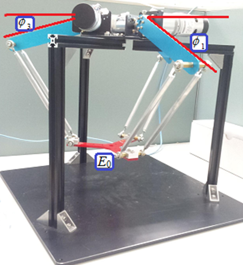
The actuators in the robot are DC brushed motors, and each upper arm is driven by a motor mounted on the fixed base. Thus, there are totally three motors on the robot. The type number of the motor is IG-42GM, manufactured by Sha Yang Ye, Inc, Taiwan. The motor also includes a set of planetary gears with the reduction ratio 1/49, which is used to reduce the rotating speed of the motor. According to the specifications provided by the manufacturer, the rated voltage, current, torque, and speed of the motor are 12 V, 5500 mA, 18 kg cm, and 119 r/min, respectively. Besides, each motor is attached by a rotary incremental encoder, which uses two Hall-effector sensors to measure the rotating angle of the motor. Since the motor can generate five pulses each round, the accuracy of the encoder can be evaluated as 0.367°.

Robot control system

The robot is driven by three motors, and each motor is controlled by a controller, which generates a signal through a control law (e.g. PID controller) processing the encoder signal. Thus, there are three motor controllers on the robot, and the entire robot control system can be treated as a semi-closed-loop system as illustrated in Figure 5. A real-time embedded system CompactRIO, manufactured by National Instruments, Inc., USA is used as a controller module in the robot control system. The embedded system has several components as follows:

An embedded processor for communication and signal processing (eRIO 9022), which is used to process all signals and to generate signals to the motor drivers.

Three servo motor driver modules (NI 9505), which are full H-bridge brushed DC servo drive modules to directly connect the motors and to decode the signals obtained from the encoders.

A reconfigurable chassis housing the user-programmable FPGA (cRIO 9112), which is a base to connect the processor eRIO 9022 and the motor driver module NI 9505.

A graphical software LabVIEW for real-time programming, where the kinematics and dynamics of the robot are programmed through a personal computer.

A personal computer, which is used to execute the codes developed by the software LabVIEW.

Figure 5.

Hardware-in-the-loop diagram.

System identification

To design a controller for the motors, it is necessary to have a mathematical model of the motor, so the system identification will be performed to determine the motor model. Since the motor is driven by a motor driver, the motor and the drive are considered as a system, and the block diagram is shown in Figure 6. The transfer function of the system model is considered as a second-order system with a time delay, which is represented as equation (17). To perform system identification for the system, one generates multiple signals as input signals, which consist of sinusoidal functions with different frequencies and amplitudes. The signals are delivered to the system, and the rotating angles are the output signals and can be measured by the encoders. The system identification of the model is completed using the MATLAB System Identification Toolbox, and Table 2 shows the estimated system parameters.

Figure 6.

Block diagram of a motor and a driver.

Table 2.

Parameters of the system model consisting of the driver and the motor.

Parameters Motor	K_m (rad/V)	T_m₁ (s)	T_m₂ (s)
Motor 1	11.089	1.268 × 10⁻³	1.143 × 10⁻²
Motor 2	10.990	1.364 × 10⁻³	1.108 × 10⁻²
Motor 3	9.768	1.000 × 10⁻³	1.037 × 10⁻²

Experimental and simulation results

This section demonstrates the tracking control using the proposed control approaches presented in “Model-based tracking control” section, where the reference signal of the control loop is a prescribed trajectory of the end effector. First, the PID controller will be used in the system control loop, where the controller parameters will be determined based on the motor models, which are identified in “System identification” section, using the Ziegler–Nichols tuning method and the software Simulink PID controller. Secondly, the numerical simulations will be performed. Thirdly, to demonstrate the proposed approaches presented in “Tracking control” section, the path planning is performed based on a quintic polynomial to design a trajectory for the end effector. Finally, the tracking control is completed based on the proposed control approaches and the path planning. The experimental and simulation results are presented, where the experimental work has been introduced in “Experimental Delta robot” section.

PID controller

The controller law applied to the Delta robot is a PID controller, and the procedure of the controller parameters is illustrated as follows:

A step function is selected as a reference command and is applied to the control system for a single motor.

The Ziegler–Nichols tuning method is applied to obtain a set of reference parameters. The Ziegler–Nichols tuning method first performs an experiment to reach the critical stability and then applies some empirical formula to obtain the controller parameters.

The obtained controller parameters are applied to numerical simulations of the robot based on the identified motor models presented in “System identification” section.

The software, Simulink PID controller, is utilized to fine-tune the parameter. Since the obtained controller parameters are based on a single-motor experiment, its performance might not be suitable for the robot.

The procedure is repeated in order to obtain the controller parameters for the other two motors.

Since the input of the controller for the position- and torque-based control systems is different, the PID controller parameters are different, which are listed in Table 3.

Table 3.

PID controller parameters.

Controls	Position-based control			Torque-based control
Controller parameters	K_P	K_I	K_D	K_P	K_I	K_D
Motor 1	0.79302	0.04091	0.38869	0.88009	0.10633	0.28262
Motor 2	0.68921	0.03551	0.40911	0.73113	0.18891	0.27901
Motor 3	0.66412	0.02984	0.39674	0.79409	0.09891	0.31971

Numerical simulations

One utilizes the software Simulink to perform the numerical simulations based on the block diagrams proposed in Figure 3, and the Simulink block diagram is shown in Figure 7. Note that the diagram includes both the position- and torque-based control systems. The procedure to perform the simulations is listed as follows:

read all command motor angles,

simultaneously perform both the position- and torque-based control,

deliver the command and output motor angles to the PID controller,

achieve the feedback control, and

show the output motor angle signals.

Figure 7.

Block diagram of performing numerical simulation through Simulink.

The simulation results are combined with the experimental results as shown in Figures 8 to 17.

Figure 8.

Active joint angles (a) φ₁₁, (b) φ₁₂, and (c) φ₁₃ by the position-based control.

Figure 9.

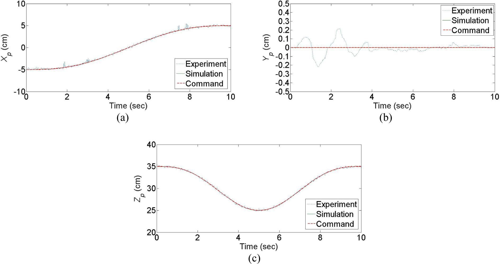
Coordinates of the end effector (a) X_p, (b) Y_p, (c) and Z_p by the position-based control.

Figure 10.

Applied torques of (a) motor 1, (b) motor 2, and (c) motor 3 by the position-based control.

Figure 11.

Velocities of the end effector (a) dX_p/dt, (b) dY_p/dt, and (c) dZ_p/dt by the position-based control.

Figure 12.

Accelerations of the end effector (a) $d^{2} X_{p} / d t^{2}$ , (b) $d^{2} Y_{p} / d t^{2}$ , and (c) $d^{2} Z_{p} / d t^{2}$ by the position-based control.

Figure 13.

Active joint angles (a) φ₁₁, (b) φ₁₂, and (c) φ₁₃ by the torque-based control.

Figure 14.

Coordinates of the end effector (a) X_p, (b) Y_p, (c) and Z_p by the torque-based control.

Figure 15.

Applied torques of (a) motor 1, (b) motor 2, and (c) motor 3 by the torque-based control.

Figure 16.

Velocities of the end effector (a) dX_p/dt, (b) dY_p/dt, and (c) dZ_p/dt by the torque-based control.

Figure 17.

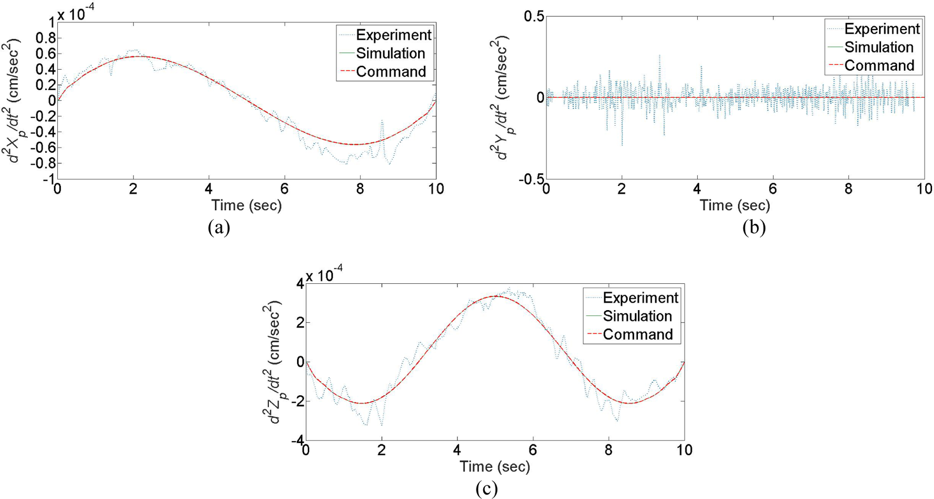
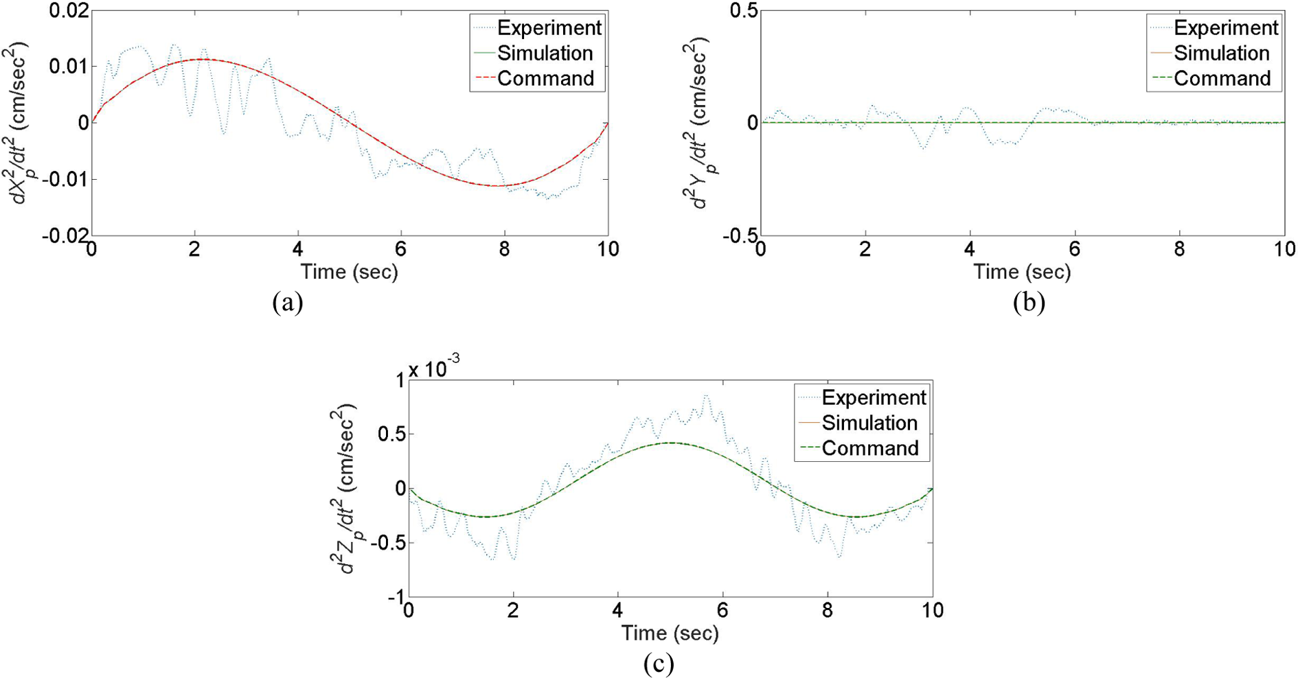
Accelerations of the end effector (a) $d^{2} X_{p} / d t^{2}$ , (b) $d^{2} Y_{p} / d t^{2}$ , and (c) $d^{2} Z_{p} / d t^{2}$ by the torque-based control.

Path planning

In this section, one intends to mimic the pick-and-place task of the Delta robot. The coordinates of the initial and final positions are selected as (X₀, Y₀, Z₀) = (−5, 0, 35) and (X_f, Y_f, Z_f) = (5, 0, 35) cm, respectively. In addition, the highest point is specified at (X_m, Y_m, Z_m) = (0, 0, 25) cm. Thus, these three points form a parabolic curve on the X–Z plane, which can be expressed as $Z = a X^{2} + b X^{2} + c$ , where a = 0.4, b = 0, and c = 25. To express the equation as parametric forms, one simply defines X = u and $Z = a u^{2} + b u + c$ . Furthermore, to ensure the zero oscillations at the initial and final positions, by following the approach presented in “Path planning” section, the boundary conditions are given as $u (t_{0}) = X_{0}$ , $\dot{u} (t_{0}) = 0$ , $\ddot{u} (t_{0}) = 0$ , $u (t_{f}) = X_{f}$ , $\dot{u} (t_{f}) = 0$ , and $\ddot{u} (t_{f}) = 0$ . The initial and final time is set to be t₀ = 0 and t_f = 10 s, respectively, so the pick-and-place task will be completed in 10 s. Therefore, the coefficients a_i in equation (14) can be determined as $a_{i} = [- 5, 0, 0, 0.1, - 0.015, 0.0006]$ . Note that the planned path should be ensured within the workspace of the Delta robot and there are no singularities on the path.

Tacking control

Two control schemes, the position- and model-based controls, are applied to the Delta robot.

Position-based control

This subsection demonstrates the position-based control introduced in “Position-based control” section, and the control is applied to the Delta robot. Figure 8 shows the time responses of the active joint angles for the desired, simulation, and experimental trajectories. The results show that the simulation and desired trajectories are coincident, but the experimental trajectory is much different from them. There are some factors yielding the inaccuracy of the experimental results. First, the initial position might not be very accurate, because there are no additional sensors to ensure the initial position as desired. As observed, there are the errors about 2° at the initial position. Secondly, the dynamics of the Delta robot is not incorporated in the control system, so the inertial and gravitational effects must affect the positioning accuracy. Finally, the gearbox of the motor has backlash, and the accuracy of the encoders has only 0.367° based on the specifications of the encoders. This causes small oscillations during the entire trajectory. Thus, those factors produce the errors about 10° at the finial position. Figure 9 shows the time responses of the positions of the end effector for the desired, simulation, and experimental trajectories. The position of the end effector is obtained by performing the direct kinematics. Due to the errors of the active joint angles, the errors of the positions are around 2 cm. Figure 10 shows the time responses of the applied torques at the active joint angles. The applied torques are determined by applying the equations of the kinematics and dynamics. Similarly, there are some errors generated from the errors of the active joint angles.

To ensure the zero oscillations at the initial and final positions of the desired path, one applies the first-order central difference method to determine the velocities and accelerations of the end effector based on the positions. As expected, there will be some errors by applying the numerical method. Figures 11 and 12 show the time responses of the velocities and accelerations of the end effector. The results show that the initial and final velocities and the accelerations are zeros.

Model-based control

This subsection demonstrates the model-based control introduced in “Model-based control” section, and the control is also applied to the Delta robot. Figure 13 shows the time responses of the active joint angles for the desired, simulation, and experimental trajectories. The results show that the three trajectories are more coincident to compare with Figure 8. Figure 14 shows the time responses of the positions of the end effector for the desired, simulation, and experimental trajectories. The position of the end effector is obtained by performing the direct kinematics. The results also show that the three trajectories are more consistent to compare with Figure 9. This implies that the included dynamics in the control system can effectively reduce the positioning errors. Figure 15 shows the time responses of the applied torques at the active joint angles. The applied torques are determined by applying the equations of the kinematics and dynamics. Furthermore, Figures 16 and 17 show the time responses of the velocities and accelerations of the end effector. The results show that the initial and final velocities and the accelerations are zeros as expected.

Discussion

To show the performance of the model-based control scheme over the conventional position-based control scheme, this section demonstrates an example, which shows both the numerical and experimental results obtained by both schemes. The example mimics the pick-and-place task of a Delta robot by designing a quintic polynomial with zero velocities and accelerations at the starting and end points. The results by applying the position-based control show that the maximum errors of the active joints are around 10°. The errors also lead to the maximum positioning errors of the end effector with around 3 cm. In contrast, the model-based control has the maximum errors of the active joints and the end effector with around 3° and 0.5 cm, respectively. Since both the control schemes are applied to the same experimental equipment, one can deduce that the model-based control has a better positioning accuracy.

Conclusions

This article presents a simple model-based control scheme applied to a Delta robot, which has three translating DOFs and is driven by three rotating motors. Conventionally, the position-based control scheme is mostly applied to positioning control of robot manipulators. This control scheme converts the robot control problem to several separated motor control problems. The major disadvantage of the control scheme might not provide a good positioning accuracy due to the lack of the robot’s dynamics in this control loop. In literature, one of the model-based controls is the computed torque control, which computes applied torques based on the inverse dynamics of robots and the errors of joint angles as well as angular velocities. The proposed model-based control scheme also computes the applied torques based on both the kinematics and dynamics of robots, but the torques are utilized to calculate the errors between them and the desired torques, which is used to fulfill the feedback control. Thus, the proposed scheme is much simpler and can be treated as an indirect torque control without using torque and current sensors. This article demonstrates the simulation and experimental results by the mode-based control scheme, and the results are compared with those by the position-based control scheme. The results show that the model-based control scheme provides better positioning accuracy.

Footnotes

Declaration of conflicting interests

The author(s) declared no potential conflicts of interest with respect to the research, authorship, and/or publication of this article.

Funding

The author(s) received no financial support for the research, authorship, and/or publication of this article.

References

Maya

Castillo

Lomelí

. Workspace and payload-capacity of a new reconfigurable delta parallel robot. Int J Adv Robot Syst 2013; 10(1): 56.

Lin

Luo

Lin

. Design and implementation of a new DELTA parallel robot in robotics competitions. Int J Adv Robot Syst 2015; 12(10): 1–10.

Castañeda

Luviano-Juarez

Chairez

. Robust trajectory tracking of a delta robot through adaptive active disturbance rejection control. IEEE Trans Control Syst Technol 2015; 23(4): 1387–1398.

Ramírez-Neria

Sira-Ramírez

Luviano-Juárez

. Active disturbance rejection control applied to a delta parallel robot in trajectory tracking tasks. Asian J Control 2015; 17(2): 636–647.

Guglielmetti

Longchamp

. Task space control of the delta parallel robot. Motion Control Int Autom 2014; 337–342.

Liu

. Design and optimization of interval type-2 fuzzy logic controller for delta parallel robot trajectory control. Int J Fuzzy Syst 2017; 19: 1–17.

Dumlu

Erenturk

. Trajectory tracking control for a 3-DOF parallel manipulator using fractional-order control. IEEE Trans Indus Elect 2014; 61(7): 3417–3426.

Lin

Liu

. The implementation of smoothing robust control for a delta robot. In: 2013 Second international conference on robot, vision and signal processing (RVSP), Kitakyushu, Japan, 10–12 December 2013, pp. 208–213. IEEE.

Zhang

Liu

Guo

. Dynamic conveyor tracking control of a delta robot. In: Erian

A. Armanios

(ed) Key Engineering Materials, Vol. 679, Trans Tech Publications, 2016, pp. 43–48. Zurich, Switzerland: Trans Tech Publications.

10.

Rachedi

Bouri

Hemici

. H∞ feedback control for Parallel mechanism and application to delta robot. In: 2014 22nd Mediterranean conference of control and automation (MED), Palermo - ITALY, 16–19 June 2014, pp. 1476–1481.

11.

Ouyang

. Integrated design and PD control of high-speed closed-loop mechanisms. J Dyn Syst Meas Control 2002; 124: 522–528.

12.

Ghorbel

Chételat

Gunawardana

. Modeling and set point control of closed-chain mechanisms: theory and experiment. IEEE Trans Control Syst Technol 2000; 8(5): 801–815.

13.

Ouyang

Zhang

. Nonlinear PD control for trajectory tracking with consideration of the design for control methodology. In: 2002 Proceedings ICRA’02 IEEE international conference on robotics and automation, Vol. 4, Washington, D.C., USA, 11–15 May 2002, pp. 4126–4131.

14.

Diaz-Rodriguez

Valera

Mata

. Model-based control of a 3-DOF parallel robot based on identified relevant parameters. IEEE/ASME Trans Mech 2013; 18(6): 1737–1744.

15.

Zhang

Sheng

Davies

. Model based open-loop posture control of a parallel ankle assessment and rehabilitation robot. In: 2015 IEEE international conference on advanced intelligent mechatronics (AIM), Busan, Korea, 7–11 July 2015, pp. 1241–1246.

16.

Meng

Zhang

Song

. High-efficiency model-based control of 6-DOF parallel robot using position measurement only. In: 2013 25th Chinese control and decision conference (CCDC), Guiyang, China, 25–27 May 2013, pp. 2612–2615.

17.

Gao

Fan

Wang

. Dynamic modeling and model-based force control of a 3-DOF translational parallel robot. In: Xiao

Zhi Hu

Alan

Kin Tak Lau

(eds) Advanced Materials Research, Vol. 1006, Trans Tech Publications, 2014, pp. 609–617. Zurich, Switzerland: Trans Tech Publications.

18.

Zhang

Liu

. Dynamic analysis and model-based feedforward control of a 2-DOF translational parallel manipulator driven by linear motors. Int J Indus Robot 2013; 40(6): 597–609.

19.

Codourey

. Dynamic modeling of parallel robots for computed-torque control implementation. Int J Robot Res 1998; 17(12): 1325–1336.

20.

Codourey

. Dynamic modelling and mass matrix evaluation of the DELTA parallel robot for axes decoupling control. Proc IEEE/RSJ Int Conf 1996; 3: 1211–1218.

21.

Yang

Mei

. Motor-mechanism dynamic model based neural network optimized computed torque control of a high speed parallel manipulator. Mechatronics 2007; 17(7): 381–390.

22.

Shang

Cong

. Nonlinear computed torque control for a high-speed planar parallel manipulator. Mechatronics 2009; 19(6): 987–992.

23.

Shang

Cong

. Adaptive computed torque control for a parallel manipulator with redundant actuation. Robotica 2012; 30(03): 457–466.

24.

Masarati

. Computed torque control of redundant manipulators using general-purpose software in real-time. Multi Syst Dyn 2014; 32(4): 403–428.

25.

Tsai

. Robot analysis: The mechanics of serial and parallel manipulators. New York, USA: John Wiley & Sons, 1999.

26.

López

Castillo

García

. Delta robot: inverse, direct, and intermediate Jacobians. Proc Inst Mech Eng C J Mech Eng Sci 2006; 220(1): 103–109.

Experimental and simulation studies of motion control of a Delta robot using a model-based approach

Abstract

Keywords

Introduction

Kinematics and dynamics of a Delta robot

Kinematics

Direct kinematics

Inverse kinematics

Workspace

Singularities

Dynamics

Model-based tracking control

Path planning

Tracking control

Position-based control

Model-based control

Experimental setup

Experimental delta robot

Robot control system

System identification

Experimental and simulation results

PID controller

Numerical simulations

Path planning

Tacking control

Position-based control

Model-based control

Discussion

Conclusions

Footnotes

Declaration of conflicting interests

Funding

References