Sage Journals: Discover world-class research

Abstract

One of the main problems in mobile robotics is localization. This article aims to increase accuracy of localization of mobile robot using visual system. Mobile robot is taking images of environment containing artificial markers. Design of the markers was also one of the tasks. Markers can be used indoors and are placed on ceiling, where there is low number of other disturbing elements. They are designed to be able to split each marker into two parts—one is changeless and the second is changing with each marker. This provides an easy segmentation of all markers and then distinguishes between them easily as well. Localization is based on changes of markers angle and position in acquired images. During research of suitable algorithms, several approaches were tested to gain optimal results of localization considering time consumption and accuracy. The last part of this work deals with implementation of visual system and odometry fusion. That provides even more precise localization of the mobile robot.

Keywords

Visual system mobile robot markers fusion

Introduction

The knowledge about position and ability to localize is a fundamental task for autonomous devices in mobile robotics. There are a number of methods to solve this problem. Mainly onboard sensors like GPS, wheel odometry, inertial sensors, camera, or their fusion are used. They differ in accuracy, resolution, and real-time processing capabilities.¹ While GPS can be very useful in outdoor environment, it might lead to a significant positioning error or even impossibility of localization due to its necessary communication with space satellites affected by buildings and other physical barriers. Therefore, in indoor areas, some improvements or other methods have to be used. The main disadvantage of wheel odometry itself is that its error integrates during the operating time, so the fusion with other inertial sensors is desired. In general, the higher the accuracy of the inertial sensors is, the higher the price it costs.

If we take some inspiration from the nature, lot of creatures, including human, use their ability to see to localize itself. According to changes in the position of environment’s features, they can estimate their own change in position. This simple idea is also useful in mobile robotics. Improvement of camera sensors during last decades has been significant and with their price they have become available for almost any robotic task.

Natural landmarks might be used directly from the environment, such as corners, edges, and other special features. However, there might be a need of higher computing performance and time consumption to find the proper features.

With this in mind, several works deal with adding artificial markers into environment^2

–6 and also commercial solutions based on additional markers were released, that is, StarGazer.³ The advantage of scanning the environment and its features by the camera is that we do not need any active landmarks, which need power for their operation, for example, positioning systems with active transmitters and receiver (Wi-Fi access points, radio, light, etc.).^4
–6

Indoor localization based on visual system and passive artificial landmarks is both accurate and economical.⁷ Illumination can influence the scanned scene so the errors in estimated position might occur when the light is changed rapidly. Proposed system is dedicated to indoor industrial environments, and markers are placed on a ceiling, where influence of outdoor light is minimal and surface is usually uniform with a small number of additional features—natural landmarks. Therefore, our system uses artificial, regularly placed markers all over the surface of a ceiling. Advantages of attaching landmarks on a ceiling have already been discussed in other studies as well.⁸

The aim of the proposed work was to create simple, easy to use, and cheap system which can be easily implemented in the industrial indoor environments using basic mobile robot, laptop, and a simple additional webcam.

Markers

Location

This work deals with indoor localization of mobile robot using visual system, for example, in a room or production hall. Proposed solution is cheap and simple. It contains only basic webcam connected to PC, where algorithm runs. Camera is placed on a robot and facing to the top to avoid obstacles in its field of view. Visual system uses artificial markers placed on the ceiling of a room. They might be painted on surface or just printed on paper and then attached to the ceiling for easier manipulation in case of replacement. This type of solution can be found also at StarGazer.³ However, its control unit, camera, and algorithms are all placed in one closed device mounted on mobile robot. Our solution allows users to make changes in both hardware and software. It can run on any PC and does not need high computer power. Suitable camera is also any low-cost webcam. Mentioned location has several other advantages, such as:

Usually fixed distance between floor and ceiling, that is, fixed distance between camera and scanned surface.

One color background with little or almost no disturbing elements.

Markers are not in path of other devices.

Considering [x, y] position of robot’s center of mass in space and robot’s rotation around it of angle ϕ. Camera is placed in the center of mass and facing upward. Then from the same position, camera scans image with the same center point. Considering different rotation, there is always a circle area recorded with this point in the center (Figure 1). Placement of the markers is then based on having at least four different markers in this circle. This makes system more robust and allows some marker not to be recognized due to, for example, unexpected changes in the scene. However changes in illumination are suppress by usage in indoor industrial environments, like production halls, where ambient illumination is mostly artificial and stable. What is more, placing markers on a ceiling reduces influence of outdoor light to minimum.

Figure 1.

Position of markers and always visible ones from one position of robot with any rotation.

Markers lay in the regular grid. According to camera parameters and distance between camera and scanned surface, it is possible to compute distance between markers (Figure 2). These schemes are used later in section “Testing,” where real setup parameters are computed based on known devices.

Figure 2.

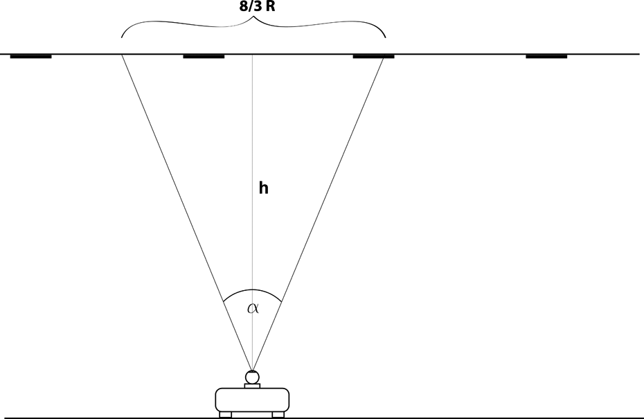
Side view: robot with mounted camera. Dependency between camera parameters, height h and scanned area.

Design

Markers were designed considering their location and surrounding. Ceiling of the room is usually white or light-colored, which is the reason for their black background. Each marker is square-shaped and divided into an imaginary grid.

First thing in image processing algorithm is to separate all markers from the surrounding, so each one should have some common features. For this reason, red circle in top-left corner is used (Figure 3). That is marker’s changeless part for easy location of each marker and so its center and rotation around perpendicular axis.

Figure 3.

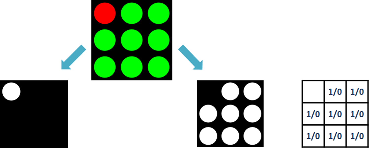
Full-covered marker. Changeless part (left) and variable part (right).

Secondly, when position and area of marker is identified, next step is to find marker’s ID. It is used to differentiate each marker and allows us to watch its position changes in the camera image. For this purpose, there are green circles placed randomly in the rest of the grid. There are (k ×k) − 1 free spots where it is possible to place green circle (Figure 3). Their position creates unique ID for each marker. A circle in spot means 1 and no circle (empty spot) means 0 in binary code. The number of different IDs without ID = 0 is then

p = 2^{[k \times k - 1]} - 1

In this case, 3 × 3 grid is used, that means k = 3, which allows us to use p = 2⁸ − 1 = 255 different markers. In comparison with StarGazer system,³ these landmarks are enriched with color. That enables us to use smaller landmarks and larger number of different ones. For example, with similar 3 × 3 matrix, landmark StarGazer offers only 31 specific IDs.

ID is computed as a binary code with the least significant bit in the bottom-right corner and then leftward in rows to most significant bit right next to the red spot. After that, ID is converted to decimal system. Figure 4 shows some examples of markers with their IDs.

Figure 4.

Examples of markers with their IDs.

Image processing

Two different approaches and image processing methods are discussed further on. The first one is low-level image processing on each acquired image based on color segmentation and finding regions. This way, the algorithm is able to find all markers and obtain their position in the image, which is later used to compute change in robot’s position by comparing values from two consecutive images. The method is supposed to be fast with low demands on computational power.

The second approach uses higher level computer vision techniques to match features between two consecutive images and from those to obtain and image transform, which is used to compute robot’s change in its position between two images. The two most common methods, speeded-up robust features (SURF)⁹ and random sample consensus (RANSAC),¹⁰ provide the desired output. No further image processing is applied. This approach is supposed to be precise and more robust because it is not strictly dependent on finding markers, it can use any other common features in two images. However, also higher power demands are expected.

At the end of this article, results from both methods are compared, and tests showed that the first approach is faster and even more precise.

Approach based on color segmentation and finding regions

For our purpose, we can consider image coordinate system is the same as robot’s coordinate system. This simplification is possible because we are only interested in changes of coordinates in the plane.

Robot’s movement is split into two parts—firstly rotation and secondly translation. As it was considered in marker’s design, their processing consists of two parts as well. Firstly, image with markers is captured by camera. Then, it is necessary to find all markers and gain their rotation. Changeless parts of markers can be used for computing robot’s rotation between two images. Ceiling, where markers are placed, and surface of robot’s movement are parallel. Therefore, change in markers rotation is the same as change in camera (robot’s) rotation. Secondly, identifying marker’s ID linked to its current position allows us to compute their changes in position from the last image. This part then enables us to gain robot’s straightforward translation.

Obtain rotation

When image is captured, first thing is to look at changeless parts of markers. That can be done by color segmentation from RGB model, which is default when image is taken. Changeless part consists of black square and red circle. So for this purpose, it is suitable to suppress green channel (G) and enhance red channel (R) simultaneously to get a grayscale image. Values were computed as R − G + B. Then, threshold and morphological operations are applied to get binary image.¹⁰ Original image and result are shown in Figure 5.

Figure 5.

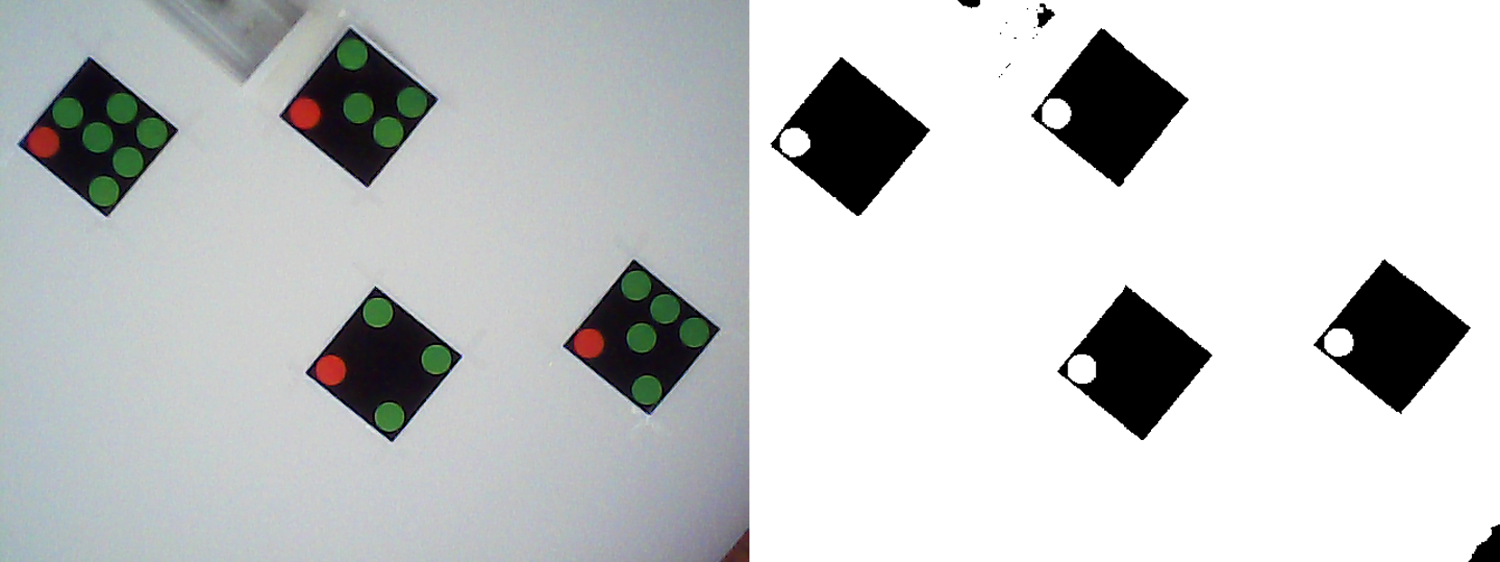
Original image (left) and result of color segmentation, thresholding, and morphological operations (right).

With a binary image consisting of 1- or 0-value pixels, it is easy to find closed regions. Pixels with value 0 belong to background and with value 1 to object (closed region).¹¹ The aim is to find objects of size which corresponds to markers. Then, using the same approach just for the object, each of them is explored to find circle in it, represents red spot in marker. Having both, center of found object and center of red circle in it, marker’s rotation can be computed (Figure 6). All of the markers are placed on the surface having the same orientation (Figure 5). However, there might be small differences between individual computed angles or some of them obtained an error, therefore, average is applied on vector of obtained angles. That value represents global rotation ϕ_im obtained from current image and its computation is expressed by the following equation

ϕ_{im} = \frac{1}{n} \sum_{k = 0}^{n} ϕ_{k}

Figure 6.

Computing marker’s rotation from known center of marker and center of circle in binary image.

where n is a number of values in angle vector and ϕ_k is its kth element (detected angle from each marker).

Difference between two consecutive images then represents which angle ϕ_rob of the robot has been turned between images’ acquisition

ϕ_{rob} = ϕ_{im (k)} - ϕ_{im (k - 1)}

where ϕ_im(k) is the current image and ϕ_im(k−1) is the previous image.

Obtain translation

Saving the position of each marker in the image is needed to obtain translation of whole image. Transformation between two consecutive images is divided into rotation and translation. As it was mentioned before, transformation between images describes movement of robot, which is split into rotation followed by translation. Rotation is obtained from segmented changeless parts of markers. Acquired angle is then used to calculate new positions of markers if only rotational movement would be applied on last image. Translation is then obtained as difference in positions of particular markers in current image and their calculated values after rotation from the last image (Δx), shown in Figure 7. Difference is calculated only in the x-coordinates. The reason is that x-coordinate of image (camera) leads in the same direction as robot’s degree of freedom for straightforward movement. Or in other words, movement is only possible in the x-axis of robot’s (image) coordinate system.

Figure 7.

Movement between two consecutive images divided into rotational and translational part. Driven distance is Δx.

As storage for marker’s positions in previous and current images, lookup table is used (Table 1). If specific marker was not situated in the last pair of photos, then it is not included in the calculation. In the lookup table, it is specified by some zero elements in coordinates and that row is subsequently omitted.

Table 1.

Lookup table with markers’ positions in previous and current images in pixels.

Marker’s ID	Position in previous image (px)		Position in current image (px)
Marker’s ID	x	y	x	y
1	0	0	0	0
2	58	120	76	105
3	0	0	43	520
⁞	⁞	⁞	⁞	⁞
254	240	356	251	349
255	0	0	0	0

Similar to rotation, translation is also obtained from each marker occurred in both images. To avoid little differences and errors, average of those values is used. Robot’s movement is measured in centimeters and this distance (d _cm) is proportional to obtained translation in pixels (t _px) as

d_{cm} = u \cdot t_{px}

Approach based on matching features between two consecutive images

Another approach using advanced computer vision techniques was also tested to compare accuracy and computing speed. It compares two consecutive images and directly computes transform matrix between them. From that, it is possible to obtain rotary and translating component of movement.

Firstly, SURF algorithm is used to find matching features in image pair.⁹ After that, they are filtered with RANSAC algorithm to remove outliers and find specific transformation.¹⁰ The output is a transformation matrix, from where translation and rotation are computed.

Figure 8 shows example of correctly matching features between two images after this set of algorithms.

Figure 8.

Pairs of matching features between two images after SURF followed by RANSAC. SURF: speeded-up robust features.

Testing

System was tested with a camera mounted on iRobot Create in two different rooms, where distance between camera and ceiling is h = 2.5 m or 3 m. The position of markers is based on schemes in Figures 1 and 2. Now in known environment, variables can be replaced by real values. Parameters of the used USB2 camera:

Resolution: 640 × 480 px

Angle: α = 30°

Angle is measured from the width of scanned area, which is 8/3R in Figure 2. Then taking image resolution, it is clear from Figure 1 that R = 240 px. Size of the marker is 20 × 20 cm, which is enough for both mentioned distances between the camera and ceiling. Table 2 shows measured properties in two mentioned environments. The way markers are placed on the surface also depends on camera parameters and its distance to surface. Apparently, a different area is scanned by camera when distance is changed, therefore distance between markers may be different as well, depending on parameters. Used setup of robot and camera is shown in Figure 9.

Figure 9.

System consists of iRobot Create and mounted camera.

Table 2.

Parameters of used setup.

Distance (m)	2.5	3
Marker size in image (px)	100 × 100	80 × 80
Size of 1 px in the image in real (u; cm)	0.2 × 0.2	0.25 × 0.25
Distance between markers in a line (320 px in image; cm)	64	80
Area covered by unique markers (m²)	26.1	40.8

There is limited number of unique markers, but area covered by markers can be unlimited. The reason is that it is possible to use marker with same ID more times, only restriction is not to place them in the area of one image. Fails in position changes calculation then may occur.

Software equipment

Camera is connected to PC via USB cable, so PC algorithm can acquire images when it is necessary, and after that, instructions are sent via Bluetooth to the robot.

Robot is equipped with odometry and able to send information about traveled distance or rotated angle from its wheels.

The PC algorithms are created in MATLAB, which offers all the necessary tools in Image Processing and Computer Vision toolbox. For both Bluetooth sending and receiving information from the robot, there is a third-party toolbox created for iRobot Create control.¹²

As it was mentioned before, movement of robot is split into rotation and translation; therefore, these two components are tested separately.

Accuracy of robot rotation according to visual system compared to robot’s odometry

Test consists of repeated request for robot to turn 90° counterclockwise. There is 20 measurement controlled by odometry compared to both visual approaches. Results of first approach based on finding regions are compared to odometry in Figure 10. On the horizontal axis, there are values of reached angles after request and on the vertical axis and there are a number of occurrences of each value after 20 requests. This visual approach consumes around 0.1–0.2 s from the image acquisition to obtaining needed value. However, several improvements could be still done to decrease time consumption like usage of camera with faster communication protocol (USB3 or PCI Express), software optimization (algorithms are currently created in MATLAB), and GPU-accelerated computing, which could make proposed algorithms real time.

Figure 10.

Compared histograms of results from odometry controlled turning (red) and from visual system based on low-level processing finding regions (green).

In Figure 11, second approach based on matching features is compared to odometry in robot’s rotation. Algorithms used in this approach are more complex and time-consuming, so as expected, computing time is longer; in this case, 0.2–0.3 s.

Figure 11.

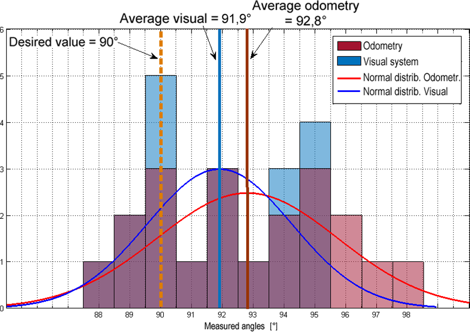
Compared histograms of results from odometry controlled turning (red) and from visual system based on SURF + RANSAC algorithm (blue). SURF: speeded-up robust features.

All histograms are with a normal distribution fit to enable comparing results easier. As shown, both visual approaches are more accurate for control of turning around specific angle than robot’s odometry. However, first approach based on finding regions obtains better results, is more precise, and less time-consuming.

As it is shown in the graphs concerning robot’s 90° turns (Figures 10 and 11), average value obtained from odometry is 92.8° (2.8° above desired value) and its variance is 8.59. Values obtained from low-level image processing method based on finding regions of markers are with the average 89.7° (0.3° under desired value) and their variance is 0.98. Values from second visual technique, obtaining transformation from matching features by SURF + RANSAC, are with the average 91.9° (1.9° above desired value) and its variance is 5.46. Both visual techniques result in better accuracy in average than odometry and also their variance proves better reliability in case of robot’s turns.

The comparison of two different vision approaches in robot’s turn control provides visibly better results in the first approach, which is based on low-level image processing based on finding individual markers in the image, storing their rotation and position, and consequently computing difference of these values between the pair of consecutive images.

Second set of measurements compares specific distance driving, again with odometry and both visual approaches separately. Desired distance is 100 cm. Figure 12 shows comparison of odometry and visual system based on finding regions. Figure 13 shows comparison of odometry and visual system based on SURF + RANSAC algorithm.

Figure 12.

Compared histograms of results from odometry controlled distance driving (red) and from visual system based on finding regions (green).

Figure 13.

Compared histograms of results from odometry controlled distance driving (red) and from visual system based on SURF + RANSAC algorithm (blue). SURF: speeded-up robust features.

In case of distance control, all approaches obtained very similar and accurate results; however, odometry got results with smallest variance. Average value of odometry controlled distance is 100.2 cm (0.2 cm above desired) and its variance is 0.69. First, visual system based on low-level processing with finding regions achieved average of 100.1 cm (0.1 cm above desired) with variance 8.31. Second, visual system using SURF + RANSAC achieved the same average value 100.1 cm (0.1 cm above desired) and its variance is 7.75.

Results show that in case of turn control, it is better to use proposed visual system, and in case of distance control, odometry is more reliable. Therefore, in the final solution, it is desired to make a fusion of both positioning methods. Matching features using SURF + RANSAC chose the most suitable features by itself; therefore, it is more power demanding and would be more suitable to the environment without known markers. In the proposed kind of task, markers are known so the image processing can only focus on their shape and appearance and ignore other features of the scene which makes it simpler. While SURF + RANSAC can occasionally find false matches in this kind of scene, another visual approach connects only centers of markers with the same ID; therefore, it is more error proof.

Odometry and visual system fusion using Kalman filter

Results obtained in the last section show there is still space for improvement. Therefore, fusion of proposed visual system and robot’s odometry was considered to improve indoor localization accuracy.

Kalman filter is widely used for sensor fusion in various forms.^13

–17 Robot is equipped with incremental encoders on its wheels as odometry. Fusion of it and visual system using Kalman filter is also discussed in several works.^16,17 This way, it is possible to increase accuracy and reduce errors in position estimation.

The discrete Kalman filter

The general aim of Kalman filter is to estimate the state x ∈ R ⁿ of a discrete-time controlled process with a measurement z ∈ R ^m .

State is described by the following equation

x_{k} = A x_{k - 1} + B u_{k - 1} + w_{k - 1}

where A is a matrix of size n × n relates the state at the previous time step k − 1 to the state at the current step k. In real, matrix A can change with every step, but here it is assumed as constant. Matrix B of size n × l describes relation between the optional control input u ∈ R ^l and the state x.¹⁸

Measurement is expressed as

z_{k} = H x_{k} + v_{k}

The m × n matrix H relates the state to the measurement z_k . Similar to A, it can change with every step, but here it is assumed as constant.

The process and measurement noise is represented by variables w_k and v_k . They are with normal probability distribution and independent of each other. Noise covariance in process (Q) and in measurement (R) are also assumed as constants¹⁸

p (w) \sim N (0, Q)

p (v) \sim N (0, R)

In the overview, Kalman filter estimates the process state at some time step and then obtains (noisy) measurements as feedback. According to this, Kalman filter equations might be split into two groups:

Time update equations: to obtain the a priori estimates for the next time step by projecting forward the current state and error covariance estimates.

(Predictor)

Measurement update equations: to obtain an improved a posteriori estimate by including a new measurement into the a priori estimate.

(Corrector)

They are both assembled into predictor–corrector algorithm (Figure 14).¹⁸

Figure 14.

Kalman filter cycle.¹⁸

Then discrete Kalman filter time update equations are

{\hat{x}}_{k}^{-} = A {\hat{x}}_{k - 1} + B u_{k - 1}

P_{k}^{-} = A P_{k - 1} A^{T} + Q

and measurement update equations are as follows

K_{k} = P_{k}^{-} H^{T} + {(H P_{k}^{-} H^{T} + R)}^{- 1}

{\hat{x}}_{k} = {\hat{x}}_{k}^{-} + K_{k} (z_{k} - H {\hat{x}}_{k}^{-})

P_{k} = (I - K_{k} H) P_{k}^{-}

Matrices A and B are from (1) and Q from (3). The state projection from time update equations coming from step k − 1 to step k.¹⁸

In the measurement update, the Kalman gain, K_k , is firstly computed. Secondly, process is measured to obtain z_k and to generate an a posteriori state estimate from it. The last step is to compute an a posteriori error covariance estimation P_k .¹⁸

When covariance matrices Q and R are considered as constant, then both the estimation error covariance P_k and the Kalman gain will quickly get to and remain in stabilized value. Considering that, these parameters can be computed off-line to decrease time consumption in real-time applications.¹⁸ The given knowledge is also used in Kalman filter draft for fusion of visual system and robot’s odometry in this work.

Kalman filter implementation and test

As it was mentioned in the last section, value of Kalman gain is obtained off-line. State of this system consists of two elements—change in angle and change in distance. They can be obtained from odometry as well as visual system. There are visible differences in accuracy between them discussed in the previous section. Odometry brings better results in straightforward movements (distance) and visual system based on finding regions is best for rotation (angle).

Kalman filter consists of two parts, as it was discussed before—prediction and correction. For prediction, mathematical model of the system might be used for calculating new state. Control based on odometry also uses mathematical properties of system like wheel size, distance between wheels, and number of increments of how much the wheel was rotated. This can be considered as prediction of the system state.

In the next step, correction is coming, which is made by visual system. That can “see” actual new position of the system and correct information from prediction. However, any of these models cannot tell us the actual state with 100% precision. For that Kalman gain K “decides” how much each method can be trusted.

So the actual state of the system is computed according to equation (8) using both prediction and correction and obtained Kalman gain. Let’s call state from prediction as $[\begin{matrix} ϕ_{o} \\ d_{o} \end{matrix}]$ and state from visual system as $[\begin{matrix} ϕ_{v} \\ d_{v} \end{matrix}]$ . They both are in the same format; therefore, matrix H can be ignored. The state of this particular system can be then described as follows

[\begin{matrix} ϕ \\ d \end{matrix}] = [\begin{matrix} ϕ_{o} \\ d_{o} \end{matrix}] + K ([\begin{matrix} ϕ_{v} \\ d_{v} \end{matrix}] - [\begin{matrix} ϕ_{o} \\ d_{o} \end{matrix}])

As it is visible from the equation, K has element for an angle and another element for a distance. When the element is close to 1, state from measurement has much more weight against state from prediction. This is used for ϕ computation. When the element is close to 0, prediction is trusted much more than measurement during state computation. That is used for d computation.

Fusion was implemented to the algorithm for control robot and then tested by moving in the square 0.5 × 0.5 m. Results are shown in Figure 15, where the square path is passed five times controlled by each method, then all three averages are compared in the graph. By records and corrections during movement using fusion, the system was able to adjust upcoming distance or angle and at the end get to its starting position.

Figure 15.

Comparing robot’s movement in square 0.5 × 0.5 m according to odometry (blue), visual system (green), and fusion of both using Kalman filter (yellow). Each path is average of five measurements.

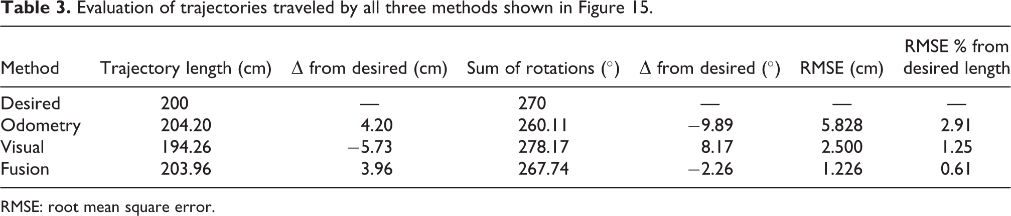
Reference frame is ground with marked desired positions in square corners. The robot was supposed to travel a desired distance along the square side to the first marked point then turn 90° and again continue straight ahead along the next side and so on using each of the three methods. Its real position was recorded in each top in regard to reference frame. Table 3 shows comparison of paths plotted in Figure 15. As it is expected, fusion of visual system and odometry brings the best results with the smallest difference from the desired path length and angle of rotation. Root mean square error (RMSE) in this case is 1.226 cm, which is 0.61% from the whole desired trajectory. Improvement using sensor fusion is visible as the robot was able to get back to its starting position. Both methods alone (odometry or visual) create error during straight movement and turning as well which at the end of path leads to bigger difference in the starting and end position. Difference in traveled distance without the use of fusion is up to 3% of whole desired distance, while using fusion it is almost five times smaller.

Table 3.

Evaluation of trajectories traveled by all three methods shown in Figure 15.

Method	Trajectory length (cm)	Δ from desired (cm)	Sum of rotations (°)	Δ from desired (°)	RMSE (cm)	RMSE % from desired length
Desired	200	—	270	—	—	—
Odometry	204.20	4.20	260.11	−9.89	5.828	2.91
Visual	194.26	−5.73	278.17	8.17	2.500	1.25
Fusion	203.96	3.96	267.74	−2.26	1.226	0.61

RMSE: root mean square error.

Conclusion

This article aimed to improve localization in mobile robotics using visual system. The goal was to create simple, cheap, and easy-to-implement robotic system as well as its own marker system. It consists of the camera mounted on a mobile robot facing upward and own marker system designed for this purpose.

Algorithm for marker recognition based on low-level image processing for finding regions of each marker in the image was created and compared with more advanced computer vision technique SURF + RANSAC used to direct computation of transformation between two images. The output from both these methods is the difference in the translation and rotation in the image, which is then computed to the difference in robot’s position between two acquired frames. Test results discussed in previous sections showed that the first provided visual algorithm can operate almost two times faster than algorithm based on SURF + RANSAC, also with smaller variance and higher accuracy during turns to desired angle. Moreover, the time consumption can still be improved by usage of camera with faster communication protocol (USB3 or PCI Express), software optimization, or GPU-accelerated computing.

Direct movement to desired distance in tests gave the best results using robot’s odometry. Therefore, it is worth to combine both methods by their fusion to compute robot’s actual position. For this purpose, Kalman filter was implemented. Kalman gain was obtained off-line to prevent system slowdown in real-time use. Results proved more precise computation of distance and rotate angle of robot’s position so the next movement could be corrected to achieve desired position. Applying this approach to the robot, robot was able to come back to its starting position after the 0.5 × 0.5 m square movement with 1.226 cm RMSE, which is almost five times improved over using robot’s odometry alone.

There are still some possible upgrades for further work, such as implementation of motion blur removal to enable correct marker recognition in higher speed of robot.^19,20

Footnotes

Declaration of conflicting interests

The author(s) declared no potential conflicts of interest with respect to the research, authorship, and/or publication of this article.

Funding

The author(s) disclosed receipt of the following financial support for the research, authorship, and/or publication of this article: Agentúra na Podporu Výskumu a Vývoja (14-0894), Req-00347-0001, and Vedecká Grantová Agentúra MŠVVaŠ SR a SAV (1/0065/16).

References

Georgiev

Allen

. Localization methods for a mobile robot in urban environments. IEEE Trans Robot 2004; 20(5): 851–864.

Chhaniyara

Althoefer

Zweiri

. A novel approach for self-localization based on computer vision and artificial marker deposition. In: Networking, sensing and control, 2007 IEEE international conference, 15 April 2007, pp. 139–144. IEEE.

User’s Guide, Localization system StarGazer for Intelligent Robots. Hagisonic, n.d. Web. 14 January 2017. http://www.robotshop.com/media/files/pdf/stargazer_user_manual_ver_04_080417%28english%29.pdf (accessed 5 October 2017).

Bejuri

WMYW

Mohamad

. Wireless LAN/FM radio-based robust mobile indoor positioning: an initial outcome. Int J Softw Eng Appl 2014; 8(2): 313–324.

Chang

Rashidzadeh

Ahmadi

. Robust indoor positioning using differential Wi-Fi access points. IEEE Trans Consum Electron 2010; 56(3): 1860–1867.

Liu

Makino

Mase

. Improved indoor location estimation using fluorescent light communication system with a nine-channel receiver. IEICE Trans Commun 2010; 93(11): 2936–2944.

Zhong

Zhou

Liu

. Design and recognition of artificial landmarks for reliable indoor self-localization of mobile robots. Int J Adv Robot Syst 2017; 14(1): 1–13. DOI: 10.1177/1729881417693489.

Park

Seo

. Autonomous position estimation of a mobile node based on landmark and localization sensor. Int J Distrib Sens Netw 2010; 104: 6.

Bay

Ess

Tuytelaars

. Speeded-up robust features (SURF). Comput Vis Image Underst 2008; 110(3): 346–359.

10.

Sonka

Hlavac

Boyle

. Image Processing, Analysis, and Machine Vision. Boston, MA: Cengage Learning, 2014.

11.

Gonzalez

Woods

Eddins

. Digital Image Processing Using MATLAB. Upper Saddle River, NJ: Pearson/Prentice Hall, 2004.

12.

Esposito

. Matlab Toolbox for the Create robot. (2011) n.d. Web. https://www.mathworks.com/matlabcentral/fileexchange/32698-matlab-toolbox-for-the-irobot-create-v2-0 (accessed 5 October 2017).

13.

Sasiadek

Hartana

. Sensor data fusion using Kalman filter. In: Proceedings of the third international conference on information fusion, 2000. FUSION 2000, vol. 2, 10 July 2000, pp. WED5–19. IEEE.

14.

Liu

Huang

Wang

. Target tracking for visual servoing systems based on an adaptive Kalman filter. Int J Adv Robot Syst 2012; 9(4): 149.

15.

Jetto

Longhi

Venturini

. Development and experimental validation of an adaptive extended Kalman filter for the localization of mobile robots. IEEE Trans Robot Autom 1999; 15(2): 219–229.

16.

Santana

Souza

Alsina

Medeiros

. Fusion of odometry and visual datas to localization a mobile robot using extended Kalman filter. In: Thomas

(ed) Sensor fusion and its applications. In: InTech, 2010, pp. 407–421.

17.

Chenavier

Crowley

. Position estimation for a mobile robot using vision and odometry. In: Proceedings of the 1992 IEEE international conference on robotics and automation, 12 May 1992, pp. 2588–2593. IEEE.

18.

Welch

Bishop

. An introduction to the Kalman filter. Department of Computer Science, University of North Carolina.” Chapel Hill, NC, unpublished manuscript, 2006.

19.

Bascle

Blake

Zisserman

. Motion deblurring and super-resolution from an image sequence. In: Computer Vision—ECCV ‘96. ECCV 1996. Lecture Notes in Computer Science (eds Buxton

Cipolla

), vol. 1065, 1996, pp. 571–582. Berlin, Heidelberg: Springer.

20.

Nayar

Ben-Ezra

. Motion-based motion deblurring. IEEE Trans Pattern Anal Mach Intell 2004; 26(6): 689–698.