Sage Journals: Discover world-class research

Abstract

A classifier training methodology is presented for Kapvik, a micro-rover prototype. A simulated light detection and ranging scan is divided into a grid, with each cell having a variety of characteristics (such as number of points, point variance and mean height) which act as inputs to classification algorithms. The training step avoids the need for time-consuming and error-prone manual classification through the use of a simulation that provides training inputs and target outputs. This simulation generates various terrains that could be encountered by a planetary rover, including untraversable ones, in a random fashion. A sensor model for a three-dimensional light detection and ranging is used with ray tracing to generate realistic noisy three-dimensional point clouds where all points that belong to untraversable terrain are labelled explicitly. A neural network classifier and its training algorithm are presented, and the results of its output as well as other popular classifiers show high accuracy on test data sets after training. The network is then tested on outdoor data to confirm it can accurately classify real-world light detection and ranging data. The results show the network is able to identify terrain correctly, falsely classifying just 4.74% of untraversable terrain.

Keywords

Planetary rovers planetary exploration neural networks autonomous navigation LiDAR classification

Introduction

In robotics, there is a current focus on increasing autonomy, so that less and less human interaction is necessary. Autonomous navigation is especially important in planetary exploration, where human communication is limited by the large distances between Earth and potential places to explore, such as Mars.¹ Moreover, in tasks such as mining,² search and recovery³ and rescue operations,⁴ the ability for an autonomous rover to understand and classify its surroundings is of utmost importance.⁵ For these reasons, a neural network classification system for light detection and ranging (LiDAR) was investigated and is presented in this article.

Kapvik, a planetary micro-rover prototype built for the Canadian Space Agency, is one such rover and is pictured in Figure 1. The rover is required to make large autonomous drives over unknown terrain, with limited computational power. The rover makes use of a simultaneous localization and mapping (SLAM) algorithm called FastSLAM 2.0⁶ that works in tandem with a D* path planning algorithm⁷ that includes terrain traversability costs similar to the algorithm demonstrated in the study by Ishigami et al.⁸ To achieve this, both LiDAR and stereocamera system are employed for use in different scenarios (such as night and day, respectively) or together. This article will detail the way in which a classifier is trained to robustly classify the traversability of terrain using the Kapvik rover’s LiDAR measurements.

Figure 1.

Kapvik micro rover.

For use as an input in path planning algorithms, it is important to classify LiDAR data as traversable or untraversable. A LiDAR scan will typically contain at least tens of thousands of data points.^9,10 In the case of Kapvik’s LiDAR, each data point contains a measurement of range, bearing and tilt. These large data sets are usually unevenly distributed, noisy, contain occlusions and spurious range data due to edges on objects and moving objects.¹¹ There must be a way for the autonomous system to differentiate which part of the scan constitutes an obstacle (i.e. untraversable) and which part can be safely navigated over (i.e. traversable). Creating a simple $2 \frac{1}{2}$ -dimensional elevation map and an expert rule-based system that computes traversability based on estimating height and slope has limitations due to incomplete and uncertain sensor data.^11
–13 More complex maps that include information such as surface normal estimation are computationally complex to compute.¹⁴ Classifiers such as neural networks can handle these issues in a robust and natural way and therefore a neural network has been used for this article.

Neural networks are often used to solve classification problems.^15
–17 They have been applied in speech recognition, character recognition and signal processing problems. It has been shown that neural networks can be viewed as universal approximators, and it has been demonstrated that a single hidden layer neural network can approximate any continuous function with support in a unit hypercube.¹⁸ Neural networks would seem worthy of investigation for the three-dimensional (3D) LiDAR classification problem. Work has been done by other researchers on classifying aerial LiDAR data that generate elevation maps of limited resolution,^19,20 and some significant work has been done in the case of 3D LiDAR from a rover perspective^{4,9,10,21
–23} and more specifically other types of classifiers such as Markov random fields,²⁴ Bayesian classifiers,²⁵ support vector machines (SVMs)²⁶ and fuzzy modelling.¹¹ Hata et al. successfully use a neural network to do such classification.²⁷ More recently, convolutional neural networks have gained attention for their ability to correctly classify images that nears or exceeds human level accuracy.²⁸ These types of networks have been adapted for use with 3D LiDAR data to detect vehicles²⁹ and other objects.³⁰ Extending classification to other metrics like lithological information is also possible using LiDAR intensity data.³¹ In planetary robotics, much work has focused on terrain parameter estimation³² and classification³³ relying on measurements from interoceptive sensors as the rover drives over terrain. Exteroceptive measurements have also been included in a self-supervised classification system.³⁴

What this article contributes is an easily adaptable training system that can be applied to a wide range of terrain types and avoids time-consuming hand-labelled target scans to be used in classifier training. For the purposes of this article, the training system has been applied to a simple multilayer perceptron (MLP) neural network. While many classifiers could be chosen, neural networks are currently the state of the art in pattern recognition and machine learning,³⁵ and the potential to expand our network model to some of the more recent developments in the literature is possible. It makes use of more information from LiDAR scans than has been used in previous examples and includes information such as the rover’s estimated pose. At the same time, using a neural network to assess raw data, computationally complex tasks such as surface normal estimation are not needed to compute traversability. The neural network presented also seamlessly incorporates different point cloud densities and sensor noise attributes. An effort has been made to keep the overall neural network structure simple, allowing easy adjustment to the inputs and outputs.

In ‘Neural network development’ section, the neural network structure is explained along with the methodology for training. The LiDAR configuration and simulation used to train the neural network is explained in ‘LiDAR configuration and terrain simulation’ section. The performance of several other classifiers trained on this data is compared to the neural network and test results using the neural network in a real-world environment are presented in ‘Results’ section.

Neural network development

The neural network structure presented here is an MLP neural network.¹⁵ The MLP was chosen for its simplicity and to test the concepts presented in this article but these concepts could easily be extended to other classifiers and was tested on a variety available in MATLAB^®.³⁶ An MLP has an input layer, output layer and in-between one or more so-called hidden layers as shown in Figure 2. Neurons are connected in layers by weighting factors that are represented by lines. The input layer neuron values are multiplied by the weighting factors, and the result is summed with all other weighted input neuron values as the input to an activation function in the next layer of neurons. The activation function used in this article is the sigmoid function

Figure 2.

Multilayer perceptron neural network.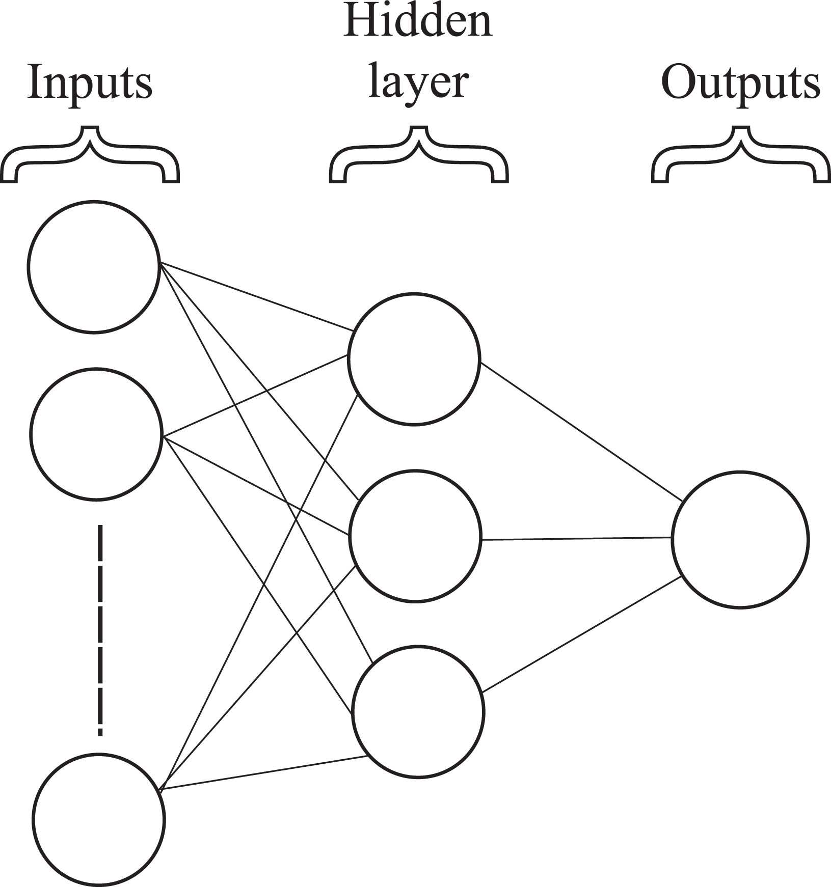

f (x) = \frac{1}{1 + e^{- x}}

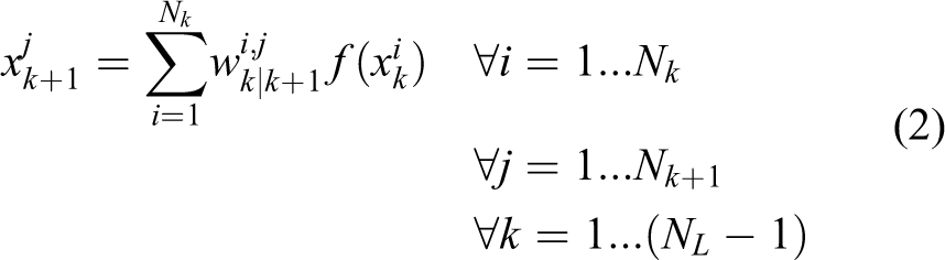
where x is the summation of all weighted neuron outputs from the previous layer. This constrains the output of the function to a value between 0 and 1. The weight that connects the ith neuron output, $f (x_{k}^{i})$ , in the kth layer to the jth neuron input in the (k + 1) layer is denoted as $w_{k | k + 1}^{i, j}$ . The input to the jth neuron in the (k + 1) layer is then computed as

\begin{matrix} x_{k + 1}^{j} = \sum_{i = 1}^{N_{k}} w_{k | k + 1}^{i, j} f (x_{k}^{i}) & \forall i = 1... N_{k} \\ \forall j = 1... N_{k + 1} \\ \forall k = 1... (N_{L} - 1) \end{matrix}

where N_k is the number of neurons in the kth layer and N_L is the total number of layers in the network.

Neural networks must be trained so that the weighting factors produce an output that is expected based on the initial input to the network. To avoid the need for the collection of large data sets and subsequent manual classification, the network undergoes training on a simulated data set representing LiDAR scans of various terrains and is shown to generalize well enough that when presented with new measurements from actual outdoor environments, it will correctly classify the terrain. What follows is a detailed description of the neural network input, output and training formulation.

Cell grid

As demonstrated in the study by Hata et al.,²⁷ the points in a new set of measurements are first organized in a cell grid overlaying the map. This is done by transforming the measurements into the global reference frame based on the estimate of the rover pose and then assigning each point to a cell.

Each cell represents a certain area of the map with a and b denoting the row and column index, respectively, starting from bottom left as shown in Figure 3. Some associated values are assigned to each cell based on the LiDAR measurements contained within it. The dimensions of each cell are chosen to be approximately the diameter of a rover wheel, as this is the typical definition of an untraversable obstacle for a rocker-bogie type rover.³⁷

Figure 3.

Cell grid to partition LiDAR scans. LiDAR: light detection and ranging.

For instance, if a cell that covers the range of points within 3–3.1 m in the x- and y-directions is selected, all points that fall within this range are considered. The values the cell takes on include things such as the mean height in comparison to the rover’s estimated height, the variance of the features in the z-direction or the difference between the maximum and minimum positions of features in the z-direction.

The neural net classifies each cell in the grid based on these inputs. To train the neural net, a set of measurements that are already classified are presented to the neural network, and based on the difference between its output and the known classification, the weights are adjusted as discussed in ‘Methodology for training’ section.

The number of neurons used for the hidden layers is determined empirically. There are no specific accuracy requirements, so the neural network is tested at various numbers of neurons, with the goal of being as accurate as possible using as few neurons as possible in each hidden layer.

To begin testing the neural network, the output is limited to a single neuron, with a value between 0 and 1. Different regions between 0 and 1 represent different classifications. For instance, in a binary classification, 0 represents completely traversable terrain and 1 represents completely untraversable terrain. The simplest output is assigned a classification based on the following rule

C_{a, b} = {\begin{array}{l} Untraversable & if O_{a, b} \geq 0.5 \\ Traversable & if O_{a, b} < 0.5 \end{array}

where O_a,b is the neural network output at the specified cell. If it is preferred to have a smoother gradient that captures the relative cost of traversing the terrain, the rule can simply contain more classification regions between 0 and 1 or report the output between 0 and 1 directly.

The activation function shown in equation (1) has limits of 0 and 1 as x goes to ±∞. If the network is trained for these outputs, the weights will be driven to large values that are unstable.¹⁷ Therefore, the network should be trained on less extreme values. In the case of this neural network, the output range is between 0.1 and 0.9, with traversable terrain being labelled 0.1 and untraversable terrain being labelled 0.9.

The neural net requires a relatively large and varied data set for training. This helps the neural net generalize which is important when it is presented later with unfamiliar terrain measurements. To offset the large amount of time and effort that is required to classify many LiDAR scans manually, a simulation was used to generate a set of simulated LiDAR scans belonging to randomly generated terrain. The terrain is then automatically classified as it is generated. For instance, when terrain is generated, the ground is labelled as traversable terrain, whereas rocks are labelled as untraversable. When the simulated LiDAR scans these different areas, the training set contains the correct labels for each scanned point to be used for supervised training. This constitutes an improvement over previous classification training methods that rely on manually labelled data sets. The simulation developed for this article is discussed in ‘LiDAR configuration and terrain simulation’ section.

Neural network input types

After dividing up the LiDAR range data into a cell format, various inputs are derived for each cell that will help the neural network determine what type of terrain that cell represents. While some cells are classified as empty, the ones that are not empty will contain one or more LiDAR data points. As an input, specific LiDAR data points are considered as well as characteristics of the group as a whole. Information about the rover’s pose is also used to influence how the neural network perceives a cell. Anything that might influence the way the LiDAR scanner scans the environment (e.g. rover pose) as well as may describe differences between different types of terrain (e.g. rock or sand) is potential inputs to the neural network. What follows is a brief description of each input used in the terrain classifying neural network. For the sake of simplicity, the following values are always assumed to be encapsulated within a single cell located at (a, b) in the cell grid.

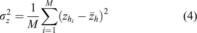
Mean height: The first input to the neural network is the cell’s mean height. The calculation for the mean height is taken as the position of the rover in the z-direction, z_r , subtracted from the mean position in the z-direction of all LiDAR data points in the cell, ${\bar{z}}_{m}$ , both with respect to the global reference frame

{\bar{z}}_{h} = {\bar{z}}_{m} - z_{r}

If the rover is operating on a two-dimensional (2D) ground plane with obstacles scattered about, this input alone could be used to determine whether a cell represented untraversable terrain or not. However, in 3D terrain, there is the potential for hills and valleys. To the rover, these might look like obstacles but are actually smooth slopes that the rover can easily traverse. To be able to differentiate between the two is of obvious importance, so other inputs from each cell must be considered.

Variance: The variance of the height of LiDAR data points in a given cell is an indication of what type of terrain it represents. Solid obstacles and terrain will have a small variance, whereas terrain that includes grass may have a larger variance in height. The variance in height for each cell is calculated as

σ_{z}^{2} = \frac{1}{M} \sum_{i = 1}^{M} {(z_{h_{i}} - {\bar{z}}_{h})}^{2}

where M is the number of points in each cell and the subscript i denotes the ith point.

Absolute height difference: The difference between the maximum and minimum height in a given cell. Data points belonging to untraversable terrain will have larger differences in height over the span of a single cell than traversable terrain.

Number of LiDAR data points: The number of points in a cell will in general be higher for untraversable terrain.

Rover orientation: The rover orientation in the pitch and roll directions has an effect on what is considered untraversable. For instance, if the rover is pitched forward, looking down a hill, an obstacle on the hill has a larger perceived height difference than if the rover sees a similar obstacle on flat terrain.

Mean height of adjacent cells: Slopes are more likely to have adjacent cells that change gradually in height than cells that include obstacles where the edges will typically have large drop-offs in height. This is illustrated in Figure 4.

Figure 4.

Comparison of adjacent cell values for slopes (left) and obstacles (right).

Methodology for training

The methods used to train a neural network are extremely important. Improper training can lead to neural networks that are not well generalized. They may perform well on a training set, but because the training set doesn’t fully represent the range of data encountered in real measurements, it may fail to generalize well enough to work in a real scenario. While part of the reason a simulation is used in training is to reduce the time required to label the training set, it is also used to increase the types of terrain encountered by the rover. For instance, if the data were obtained from a few locations in and around a university campus with the actual LiDAR, and then manually labelled, the data set might not resemble the terrain located on Mars or another common outdoor environment.

There is also a question of too much training data, where the neural net is not able to encode the information from all possibilities adequately. Using a simulation, the type and volume of terrain the neural net is trained on is easily controlled. However, simulations present new problems. The terrain generated is a smooth surface described by a polynomial, and the obstacles are polyhedron shapes. The question is whether the neural network will be able to generalize these more basic geometries from the training set to real data it receives while driving outdoors. In this article, the training and validation steps are done through simulation, and the testing set is from real-world scan data. The neural network trained on simulated data must correctly classify scans taken in the real world.

If the neural network fails on real data, the question becomes whether some fundamental information is not being given to the neural network causing it to fail or if the training set itself needs to be changed, to more accurately represent data, the rover will encounter in the real world.

The neural network presented in this article is trained using a nonlinear Kalman filter rather than the more popular backpropagation method. In the study by Singhal and Wu,³⁸ it was first shown that an extended Kalman filter (EKF) could be used to train a neural network. In the study by Ruck et al.,³⁹ it was shown that backpropagation is a degenerate form of the EKF, one in which the errors in the weights are assumed to be uncorrelated, leading to potentially less accurate results. This result and the potential to reuse nonlinear Kalman filter algorithms already developed for the state estimation algorithms of Kapvik led to its use as the training method for the presented neural network.

To properly estimate each of the weight states, the training set should be at least as large as the number of weights. For the initial training, a new surface is generated for each training set input/output pair and a measurement is taken by placing the rover in a random location. This ensures that the terrain is different in each scan. After one scan, each of the inputs is calculated and formed into the neural network input vector u _n discussed in ‘Neural network input types’ section and an output based on the untraversable label for each cell, determined by simulation, denoted as d _n. For instance, if any of the data points in a cell belong to an obstacle, the cell is labelled untraversable and d _n will be equal to 0.9.

Before training, the data set is divided into three sections: 70% of the data set is reserved for training, 15% for validation and 15% for testing. A nonlinear Kalman filter trains the weights of the neural network as shown in Figure 5 using the training part of the data set. After the training for a particular input is accomplished, the weights are passed onto the next iteration of the Kalman filter along with a new training input/output pair. To avoid overfitting, the validation set error is checked at set intervals during training. When the validation set error is determined to be rising, training ends and the network reverts to the estimated weights at the iteration where validation set error was at a minimum. The test set is used separately, after training is complete, to evaluate the performance of the neural network against other models or classifier types.

Figure 5.

Neural network trained by Kalman Filter.

EKF formulation

What follows is a short description of the design of an EKF for use in training a neural network, which shows the relation between it and the more common backpropagation training rule. It is straightforward to extend this formulation to other nonlinear Kalman filters (e.g. an unscented Kalman filter) where it is unnecessary to explicitly compute the Jacobian of the neural network model. We adopt the notation in the study by Barfoot,⁴⁰ where estimates based on a prior and the latest input are accented with a $\overset{ˇ}{(\cdot)}$ symbol and corrected estimates are accented with a $\hat{(.)}$ symbol. We constrain our belief function for the weight estimate at iteration n, ${\hat{w}}_{n}$ , to be Gaussian

p (w_{n} | {\overset{⌣}{w}}_{0}, u_{1 : n}, d_{1 : n}) = N ({\hat{w}}_{n}, {\hat{P}}_{n})

where ${\overset{⌣}{w}}_{0}$ is the initialized weight value prior, and ${\hat{P}}_{n}$ is the covariance of the weight estimate. The noise variables for the inputs, ω _n, and measurements, ν _n , are also treated as Gaussian with diagonal covariance matrices Q _n and R n , respectively

ω_{n} \sim N (0, Q_{n})

ν_{n} \sim N (0, R_{n})

The process and measurement models are defined as

w_{n} = f (w_{n - 1}) + ω_{n}

= w_{n - 1} + ω_{n}

d_{n} = b (w_{n}, u_{n}) + ν_{n}

where b is the neural network model output. The EKF prediction and measurement correction steps can then be written as

Prediction : {\overset{⌣}{P}}_{n} = F_{n - 1} {\hat{P}}_{n} F_{n - 1}^{T} + Q_{n}

{\overset{⌣}{w}}_{n} = {\hat{w}}_{n - 1}

Kalmangain: K_{n} = {\overset{⌣}{P}}_{n} B_{n}^{T} {(B_{n} {\overset{⌣}{P}}_{n} B_{n}^{T} + R_{n})}^{- 1}

{\hat{P}}_{n} = (1 - K_{n} B_{n}) {\overset{⌣}{P}}_{n}

Correction: {\hat{w}}_{n} = {\overset{⌣}{w}}_{n} + K_{n} (d_{n} - b ({\overset{⌣}{w}}_{n}, u_{n}))

Because the process model in the prediction step follows a random walk model (i.e. static + noise), F _{n − 1} is simply the identity matrix. The Jacobian of the network model, B, results from linearizing the network at the current weight estimates

B_{n} = {\frac{\partial b ({\overset{⌣}{w}}_{n}, u_{n}, ν_{n})}{\partial w_{n}} |}_{{\overset{⌣}{w}}_{n}, u_{n}, 0}

As shown in the study by Ruck et al.,³⁹ the backpropagation training rule reduces to

Δ w = η (d_{n} - b ({\overset{⌣}{w}}_{n}, u_{n}, 0)) B_{n}

where η is the so-called learning rate, and similarly the EKF algorithm reduces to

Δ w = a p (d_{n} - b ({\overset{⌣}{w}}_{n}, u_{n}, 0)) B_{n}

if the following assumptions are made: (1) P _n = p I and (2) ${(B_{n} {\overset{⌣}{P}}_{n} B_{n}^{T} + R_{n})}^{- 1} = a I$ . Therefore, the update in the weight estimates is the same as the backpropagation training rule with η = ap. Given the first assumption, the errors in the weights are uncorrelated (P remains diagonal) which is obviously untrue as the weights in the upper layers contribute to the derivatives of the network with respect to the weights of the lower layers. The ability of the filter to modify K over time is also lost, and therefore the size of the update at each iteration will remain the same. Without going into the derivation here, it is also shown in the study by Ruck et al.³⁹ that the conditions to satisfy the second assumption are not generally met. It’s clear that backpropagation is not using all the information available to update the weights.

In the study by Chernodub,⁴¹ it is shown that Kalman filters have comparable performance to the second-order batch optimization methods (e.g. gradient descent) for training neural networks used in classification problems, with the added benefit of being easily run in a real-time fashion. However, as shown in the study by Puskorius and Feldkamp,⁴² the computational complexity of an EKF estimating a neural network with p outputs and s weights is O(ps ²) and its storage requirements are O(s ²), which for large neural networks makes the EKF much more computationally demanding than backpropagation. To remedy this, a decoupled EKF was introduced that decouples weights into mutually exclusive groups, which results in a covariance matrix that is more sparse and block diagonal. The number of groups can be tuned between one and s groups, where one group is equivalent to a standard EKF, encompassing the entire covariance, and having s groups assumes the errors in the weights are uncorrelated and is equivalent to backpropagation. One suggested grouping is to group weights that share a single input node with each other. This allows for flexibility when applying this algorithm to different scenarios, for example, training offline with a powerful computer versus online on different rover platforms with different computational abilities. It is also possible to use other nonlinear Kalman filtering algorithms for this purpose, including ones that do not require explicit calculation of the Jacobians for each network model. For the purposes of this article, only one group was used (all weight covariances were estimated) to obtain the most accurate results, but the flexibility to tune the algorithm to our needs and to swap in nonlinear Kalman filter algorithms already developed for SLAM has proven useful.

LiDAR configuration and terrain simulation

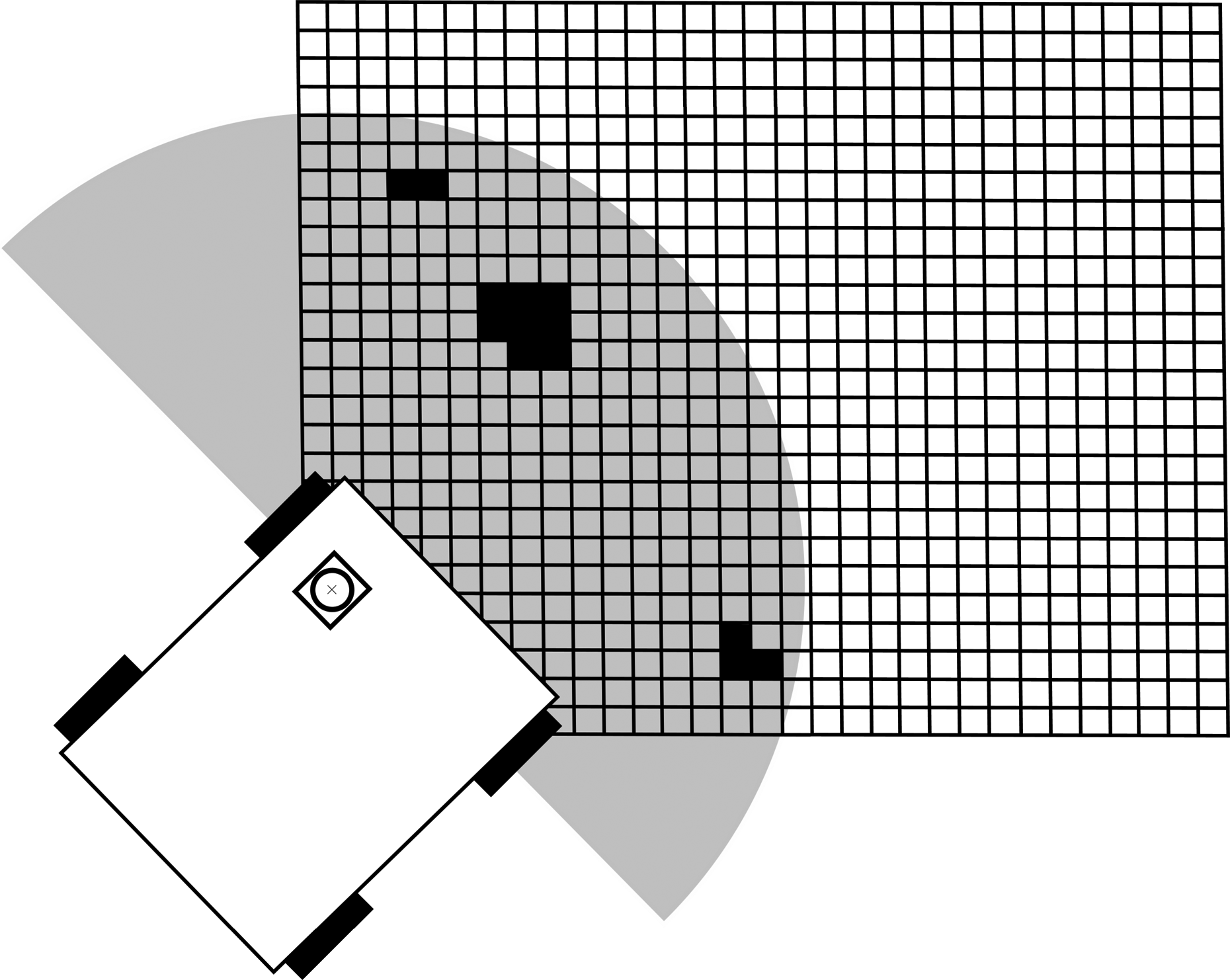
A typical LiDAR will return a range and bearing which can be converted to a Cartesian position with knowledge of the pose of the LiDAR device. To avoid the expense of a 3D LiDAR scanner, 2D LiDAR scanners can be made to tilt about an axis using a tilt device, and at set intervals take 2D scans as shown in Figure 6. The combination of 2D scans and tilt intervals can be used to create a 3D scan that approximates scans that a 3D scanner creates. The expected operating environments and stop and go nature of the micro-rover Kapvik allow the use of scans taken with the rover in a stationary pose, devoid of any moving objects such as people or vehicles.

Figure 6.

2D scanner used for 3D scans. 2D: two-dimensional.

For this article, a Directed Perception PTU D46 (FLIR Systems, Burlingame, California, USA) is used as the tilt unit and a Hokuyo URG-04LX (Hokuyo Automatic Co., Ltd., Osaka, Japan) range finder. The LiDAR and tilt unit are mounted together on a Pioneer rover centred at the front of the rover as shown in Figure 7. The Pioneer rover was used for testing the algorithm while Kapvik was being built; however, the scans taken by the LiDAR sensor are almost identical for either platform.

Figure 7.

Pioneer rover with tilt unit and LiDAR attached. LiDAR: light detection and ranging.

To train the neural network, a simulation developed in MATLAB was used. The simulation models 3D terrain such as sloping hills and rocks, a rover traversing over this terrain and a LiDAR measuring the terrain from the rover’s location. Note that training is done offline, prior to the robot operating in the field; therefore, the computational cost of such a simulation is less critical. It should be noted that other methods of simulating the scenario, such as the Gazebo simulator⁴³ would be equally appropriate.

3D terrain

For the purposes of Kapvik, there are two basic types of terrain. The first is traversable terrain, which represents sloping hills and valleys as well as flat surfaces. In the real-world tests done, this includes surfaces such as sand, cement and grass. The second type is untraversable terrain. This includes objects such as rocks, trees, bushes and other objects that are laying on the ground terrain and are larger than one Kapvik wheel diameter in height above the surface.

The ground terrain is constructed by randomly generating points in two dimensions and convolving this with a Gaussian filter using the method outlined in the study by Garcia and Stoll.⁴⁴ The convolution is achieved using the fast Fourier transform function in MATLAB. A polynomial is then fitted to the result such that

z_{T} = f (x, y)

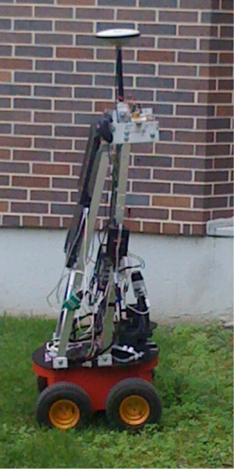
where z_T is the height of the terrain in the global reference frame at the surface position located at (x, y). By randomly producing the 2D set of surface points and the parameters of the Gaussian filter, a different ground shape is generated each time a training set is created, as shown in Figure 8(a).

Figure 8.

Examples of simulation used to train classifier. (a) Simulated rover driving over sloping terrain. (b) Simulated LiDAR scan.

To generate obstacles, a convex polyhedron model is used for the purpose of speeding up LiDAR simulation. Unlike an open-ended surface, closed surfaces such as rocks can be represented by a polyhedron. Efficient ray tracing operations for polyhedron are well established in computer graphics literature and the method used in the study by Haines⁴⁵ is used for this work. This allows the creation of many such objects in a given map. These objects are varied in size and location randomly, with a mean Z position of zero in relation to the ground it resides on. Much like rocks in nature, some of the polyhedron resides below the surface it is laying on.

The end result of these two processes is a terrain with varying degrees of slope and a random distribution of obstacles at different heights above the ground terrain that are untraversable as shown in Figure 8(a). From the viewpoint of a LiDAR, this type of terrain closely matches the type of terrain encountered in an outdoor environment. In addition to these two main types of terrain, one can adjust the simulation to account for trees using cylindrical shapes instead of polyhedron shapes. To simulate grass or bushes, adding variance to the measurements generated from designated areas of traversable or untraversable terrains will differentiate these terrains from the ‘regular’ terrain in a realistic way.

Rover model

The rover used in this simulation is modelled after a differential drive rover such as the Pioneer rover that was used for some of the outdoor tests. Kapvik may be approximated similarly as it uses skid steering and the motor controllers drive each side of wheels nominally at the same speed. A differential drive rover forward kinematic model was simplified to a unicycle model, with inputs of $\vec{v} (t)$ and $\vec{ω} (t)$ for linear and angular velocity, respectively, at time t. Differential drive rovers are generally capable of turning in place so this simplification is close to actual kinematic behaviour.

After the rover moves through one time step, the pose is adjusted to conform to the terrain beneath it. To simplify the simulation, it has been assumed that the surface is smooth and that the wheels are always in contact with the surface at a single point of contact. In the study by Tarokh and McDermott,⁴⁶ a kinematic model is developed to determine the rover wheel configuration given the constraints of the rover’s x- and y-position and its heading, ϕ_z , that has been adjusted here for use on both differential drive and rocker-bogie vehicle mobility types.

In addition, at each time step, the simulation determines slope and height of the surface at the global x- and y-position of each of the rover’s wheels. Based on the slope and height of the surface mesh under each wheel, the pose of the rover is optimized under the constraints of its position and its current direction using the fminsearch function in MATLAB. The end result is shown in Figure 8(a). To simulate bumpy and uneven terrain, some noise is added to the control input vector.

For the purposes of the simulation, the rover is started at a random position above the randomly generated terrain. It is in general placed in a location somewhat close to an obstacle so that at least one valid scan containing both traversable and untraversable terrain is taken, but this can be adjusted. The trajectory the rover takes can be changed to avoid obstacles using a path planning algorithm, but for the initial tests, the rover drove a limited distance so this was unnecessary.

To accurately simulate a real-world scenario, the rover’s pose in the global reference frame is estimated using FastSLAM 2.0.⁶ The estimated pose and uncertainty is used as one set of inputs to the neural net, rather than the ‘true’ simulated rover pose. The measurements supplied to the FastSLAM 2.0 algorithm include a simulated IMU that can observe the rover’s pitch and roll, a sun sensor that observes heading and the rover’s LiDAR measurements, which are used to track features from multiple viewpoints and allow the rover to observe the position of those features and its own pose in the global reference frame. Each measurement is summed with random Gaussian noise based on sensor specifications.

LiDAR model

To simulate LiDAR scans, a set of ‘rays’ is generated, each ray representing a single LiDAR measurement direction. In our case, this consists of a set number of 2D scans at each tilt interval. Each ray is calculated in its parameterized form based on the position of two points. The first point is the position of the LiDAR sensor and the second point is defined by the tilt and bearing angles as well as the maximum range of the LiDAR.

The next step is to determine the intersection points, if any, between these rays and the surface mesh that represents the ground as well as the polyhedrons representing objects. The ultimate goal is to determine, for each ray, the intersection point that is the closest distance to the LiDAR. To do this, the intersection points are calculated for the ground first. A system of nonlinear equations is set up using equation (19) and parameterized line equations. Using MATLAB’s fmincon function, a solution for the intersection point is found for each ray within the boundaries of the LiDAR field of view. These intersection points are then compared to any intersection points with untraversable terrain.

The distance of each intersection point from the LiDAR head position corresponds to the range measurement. The intersection point with the smallest distance from the rover is then selected as the measurement. After this selection, Gaussian noise is added to the range measurement. The bearing and tilt measurements are predefined by the resolution of the LiDAR bearing and the tilt unit. An example of the simulated LiDAR scan of an environment is shown in Figure 8(b).

Results

With the neural network developed in ‘Neural network development’ section and the simulation in ‘LiDAR configuration and terrain simulation’ section, training of a neural network can be accomplished. The algorithm was run on a test set generated by the same simulation as the training and validation sets. The neural networks were trained with all inputs and the binary outputs discussed in ‘Neural network development’ section. The grid cell size was set to 0.1 × 0.1 m² and a varying number of hidden layers and their corresponding number of neurons were tested on the same data set. The maximum number of neurons was limited to 32 and the maximum number of hidden layers was limited to 3 to avoid high computational cost. By testing all possible permutations, it was determined that the best performance was obtained using 2 hidden layers, with 16 neurons each.

For comparison, the same training, validation and test sets from simulation were used to train and evaluate other popular classifier options using the classification learner tool available in MATLAB. The confusion matrices for the top four performers are shown in Figure 9 which shows that the neural network is 90.2% accurate and performs comparably to the algorithms in MATLAB: fine Gaussian SVM at 89.0%, fine K-nearest neighbour (KNN) at 92.5% and complex decision tree at 80.7%. While these results show that the fine KNN algorithm performs slightly better than the presented neural network algorithm, the neural network algorithm was chosen for its flexibility to tune for performance as discussed in ‘EKF formulation’ section and to leave open the option to expand the algorithm to more complex network architectures. However, this analysis shows that the proposed training method is valid for a wide array of classification algorithms.

Figure 9.

Performance of several classifiers on test data set. (a) Neural network. (b) Fine Gaussian SVM. (c) Fine KNN. (d) Complex tree. SVM: support vector machine; KNN: K-nearest neighbour.

Outdoor tests

The results in Figure 9 show that the neural network and other classifiers have been successfully trained to differentiate terrain (in this case as traversable or untraversable) in a simulated environment with 90.2% accuracy. The trained neural network was then tested on actual outdoor data taken with the Hokuyo LiDAR scanner. The goal was to output scans that separate traversable and untraversable terrain, verified by visually inspecting each classification and comparing to pictures taken at the same time and place. The untraversable terrain that has been classified can then be used as an input to path planning or data association problems.

Scans were taken on the Carleton University campus. The environments chosen included large boulders, sidewalks, grass, trees, shrubs and brick walls. This presented a number of varied terrain types for the neural network to classify. An example of a classified scan is shown in Figure 10 with an original scan, classified scan and picture taken from slightly above the LiDAR’s point of view. Lightly coloured points represent traversable terrain, whereas untraversable terrain is darkly coloured. In Figure 10(c), the large boulder to the left seen in Figure 10(a) can be seen to be classified correctly as untraversable, along with the small rock shown to the extreme right of the image. The boulder that appears in the middle-right of the image does not appear in the LiDAR scan due to its distance from the rover and the limited range of the Hokuyo range finder.

Figure 10.

Comparison of original and classified LiDAR scans on Carleton University campus. (a) Photograph of scene. (b) Original scan. (c) Classified scan with untraversable cells darkly shaded. LiDAR: light detection and ranging.

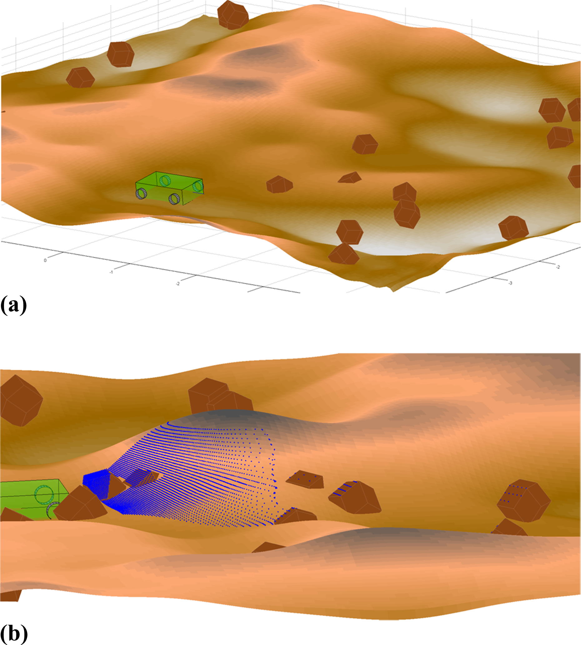
Petrie Island beach near Ottawa, Canada was used as a testing ground for Kapvik’s chassis so the LiDAR classification was tested on this terrain as well. This terrain is more similar to a Martian environment than the other outdoor measurements taken at Carleton’s campus.

A SICK LMS LiDAR (SICK AG, Waldkirch, Germany) and Husky (Clearpath Inc., Waterloo, Canada) rover were used instead of the Hokuyo range finder and Pioneer rover so the range of each scan was much larger. To test a variety of features in the laser scans, sand was shovelled and shaped to form slopes. In addition, rocks and a bucket were placed in front of the rover to act as obstacles. The sloping terrain should not be identified by the rover as untraversable in most cases, whereas the rocks and bucket should. A picture of the scan area is shown in Figure 11(a) with the slopes and obstacles labelled. A scan was taken and classified over this area. As in the previous scans, the lightly coloured points represent traversable terrain and darkly coloured points represent untraversable terrain. The corresponding shapes in the classified scan are labelled in Figure 11(b). The plot shows that all features were correctly identified while leaving the sloping terrain classified as traversable.

Figure 11.

Classified scan at Petrie Island, Ottawa, Canada. (a) Photograph of scene. (b) Classified scan with darkly shaded cells indicating untraversable terrain.

To quantitatively assess the performance of the LiDAR classification, several different scans were taken at Petrie Island beach. Each of the scans had a varying rover pose and a different number of visible obstacles. The obstacles were positioned differently for each scan. Each scan was manually labelled and the LiDAR classifier output was compared to this. The results of these tests are shown in Table 1.

Table 1.

Classifier performance on Petrie Island beach data set.

Number of classified untraversable points	11,687
Number of classified traversable points	308,800
Percentage of falsely classified untraversable points	4.74
Percentage of falsely classified traversable points	0.81
Percentage of total falsely classified points	0.96

While the overall scan classification is accurate, the untraversable classification does not perform as well as traversable classification. Obstacles are generally sparsely located across a LiDAR map. The majority of the error in classification comes from the flat tops of rocks. These areas could in a sense be considered traversable leaving the steep walls of tall rocks as the true obstacle for the rover. To classify the whole rock as untraversable, a greater range of neighbouring points should be included in the neural network so this is captured in the training step. In either case, the rover will not attempt to drive over this terrain as it is surrounded by untraversable points. Incorrect classification of untraversable terrain as traversable makes up less than 1% of the untraversable points that do not originate from the tops of rocks.

The Petrie Island quantitative results were then verified by applying the algorithm to much richer data sets. In collaboration with the Canadian Space Agency and Neptec Design Group Ltd, the algorithms were tested using the integrated vision, imaging and geological mapping sensor (IVIGMS)⁴⁷ to generate dense scans of the Canadian Space Agency’s planetary emulation terrain. The scans include large boulders, sloping traversable terrain and steep cliffs. The scan pattern of the IVIGMS is unique; scans taken over longer periods of time generate denser point clouds. The classifier performed very well, despite being trained on a much different scan pattern, as shown in Figure 12. It correctly identified all major obstacles, including differentiating between rocky and traversable sloping terrain. The binary and direct outputs of the classifier are displayed in Figure 12(b) and (c), respectively. The direct output is scaled between lightly shaded and darkly shaded based on the output between 0.1 and 0.9, respectively.

Figure 12.

Classified scan at Canadian Planetary Emulation Terrain. (a) Photograph of Canadian Planetary Emulation Terrain. (b) Scan of area depicted in photograph, with cells shaded based on binary classifier output. (c) Classified scan with cells shaded based on direct classifier output.

The majority of errors in classification were cells incorrectly labelled untraversable. These cells were mostly located beyond 10 m, where the scan data were much sparser on flat terrain. A correlation between scan density and falsely classified cells can be seen in Figure 13 and on closer inspection, the scan pattern creates the illusion of occlusions where the data are sparse. For the purposes of the Kapvik rover, a 10-m range of classification is acceptable for short-term path planning; however, cell density is an input to the neural network and it is acceptable that it advises caution in areas that have not been adequately scanned.

Figure 13.

Comparison between cell density and incorrect cell classifications. (a) Cell density of Canadian Planetary Emulation Terrain scan; lightly shaded points belong to sparsely populated cells, darkly shaded points belong to densely populated cells. (b) Examples of incorrect cell classifications (darkly shaded cells within ellipses) that correlate with sparsity.

The second data set presented in the study by Anderson et al.⁴⁸ makes use of an Autonosys (Autonosys Inc., Ottawa, Canada) scanning LiDAR (with a similar scanning pattern to the LiDAR used at Petrie Island) in a gravel pit located near Sudbury, Ontario that acted as a planetary analogue shown in Figure 14. This data set contains much more extreme changes in elevation and many different types of terrain such as flat and steep terrain with small rocks and boulders scattered across it. The classifier successfully identified boulders and steep terrain as untraversable, whereas smooth terrain at the bottom of a valley is classified as traversable. The direct and binary outputs are displayed in Figure 14.

Figure 14.

Classified scan at Ethier Sand and Gravel Pit, Sudbury, Ontario, Canada. (a) Photograph of sand and gravel pit (credit: Ethier Sand and Gravel Limited). (b) Mesh fitted to mean height of unclassified cell grid. (c) Classified scan with cells shaded based on binary classifier output. (d) Classified scan with cells shaded based on direct classifier output.

Conclusion

The presented simulation-based training methodology shows significant success in traversability classification of LiDAR data, using different LiDAR sensors on different types of terrain. Through simulation, changes in LiDAR and terrain can easily be implemented and manually labelling data sets are avoided. This constitutes a major improvement over previous classification training methods that rely on manually labelled data sets, allowing a variety of terrain to be tested and doing so in a fraction of the time. The classified traversability of observed terrain can then be used by guidance and navigation algorithms such as path planning and SLAM. This will be particularly useful during missions that contain dangerous, rocky terrain like that observed during the Viking Lander, Mars Pathfinder and Mars Science Laboratory missions.

The output types and simulation complexity could potentially be expanded upon to improve classification; however, the proposed training methodology has demonstrated that it is possible to train classifiers using only simulation in the case of a planetary rover equipped with a LiDAR sensor. Building off the work in the study by Hewitt and Marshall,⁴⁹ future improvements will involve the use of LiDAR intensity measurements as additional inputs to the classifier, as they provide an additional observation of the surface normal and the object reflectivity, both indicative of different types of terrain.

Footnotes

Declaration of conflicting interests

The author(s) declared no potential conflicts of interest with respect to the research, authorship, and/or publication of this article.

Funding

The author(s) received no financial support for the research, authorship, and/or publication of this article.

References

Baumgartner

. In-situ exploration of mars using rover systems. In: Space 2000 conference, Long Beach, CA, August 2000, pp. 1–9. AIAA.

Pool

. Scan registration for autonomous mining vehicles using 3D-NDT. J Field Robot 2007; 24(10): 803–827.

Johnson

Montgomery

Matthies

. Vision guided landing of an autonomous helicopter in hazardous terrain. In: International conference on robotics and automation (ICRA), Barcelona, Spain, April 2005, pp. 3966–3971. IEEE.

Sheh

Kadous

Sammut

. Extracting terrain features from range images for autonomous random stepfield traversal. In: International workshop on safety, security and rescue robotics, Rome, Italy, 2007, pp. 1–6. IEEE.

Talukder

Manduchi

Rankin

. Fast and reliable obstacle detection and segmentation for cross-country navigation. In: Intelligent Vehicle Symposium, Vol. 2, Versailles, France, 2002, pp. 610–618. IEEE.

Montemerlo

Thrun

Koller

. Fastslam 2.0: an improved particle filtering algorithm for simultaneous localization and mapping that provably converges. In: International joint conference on artificial intelligence, Vol. 18, Acapulco, Mexico, August 2003, pp. 1151–1156. Citeseer.

Ferguson

Stentz

. Field d*: an interpolation-based path planner and replanner. Int J Robot Res 2007; 28: 239–253.

Ishigami

Nagatani

Yoshida

. Path planning and evaluation for planetary rovers based on dynamic mobility index. In: International conference on intelligent robots and systems (IROS), San Francisco, USA, September 2011, pp. 601–606. IEEE/RSJ.

Nüchter

Surmann

Hertzberg

. Automatic classification of objects in 3D laser range scans. In: Intelligent autonomous systems conference, Amsterdam, The Netherlands, March 2004, pp. 963–970. Citeseer.

10.

Granström

Schön

. Learning to close the loop from 3D point clouds. In: International conference on intelligent robots and systems (IROS), Taipei, Taiwan, October 2010, pp. 2089–2095. IEEE/RSJ.

11.

Mandow

Cantador

Garcia-Cerezo

. Fuzzy modeling of natural terrain elevation from a 3D scanner point cloud. In: International symposium on intelligent signal processing. Floriana, Malta, September 2011, pp. 1–5. IEEE.

12.

Gallant

. Neural network learning and expert systems. Cambridge, MA: MIT Press, 1993.

13.

Kasabov

. Foundations of neural networks, fuzzy systems and knowledge engineering. Cambridge, MA: MIT Press, 1996.

14.

Klasing

Althoff

Wollherr

. Comparison of surface normal estimation methods for range sensing applications. In: International conference on robotics and automation (ICRA). Kobe, Japan, May 2009, pp. 3206–3211. IEEE.

15.

Haykin

. Neural networks and learning machines, 3rd ed. Upper Saddle River, NJ: Pearson Education, Inc., 2009.

16.

Fausett

. Fundamentals of neural networks, 1st ed. New York: Prentice Hall, 1994.

17.

Masters

. Practical neural network recipes in C++. San Diego, CA: Academic Press, Inc., 1993.

18.

Cybenko

. Approximation by superpositions of a sigmoidal function. Math Control Signal Syst 1989; 2(4): 303–314.

19.

Verma

Kumar

Hsu

. 3D building detection and modeling from aerial LiDAR data. In: Computer society conference on computer vision and pattern recognition (CVPR), Vol. 2, New York City, NY, June 2006, pp. 2213–2220. IEEE.

20.

Charaniya

Manduchi

Lodha

. Supervised parametric classification of aerial LiDAR data. In: Computer vision and pattern recognition workshop (CVPRW), Washington, DC, July 2004, pp. 30–30. IEEE.

21.

Fujita

. 3D terrain measurement system with movable laser range finder. In: International workshop on safety, security & rescue robotics, Denver, CO, November 2009, pp. 1–6. IEEE.

22.

Rekleitis

Bedwani

Dupuis

. Autonomous planetary exploration using LiDAR data. In: International conference on robotics and automation (ICRA), Kobe, Japan, May 2009, pp. 2048–2053. IEEE.

23.

Pellenz

Neuhaus

Dillenberger

. Mixed 2D/3D perception for autonomous robots in unstructured environments. In: RoboCup 2010. Singapore, June 2011, pp. 303–313. Springer-Verlag.

24.

Wellington

Courville

Stentz

. Interacting Markov random fields for simultaneous terrain modeling and obstacle detection. In: Robotics: Science and systems. Cambridge, MA, June 2005, pp. 1–8. The MIT Press.

25.

Lalonde

Vandapel

Huber

. Natural terrain classification using three-dimensional ladar data for ground robot mobility. J Field Robot 2006; 23(10): 839–861.

26.

Wurm

Kümmerle

Stachniss

. Improving robot navigation in structured outdoor environments by identifying vegetation from laser data. In: International conference on intelligent robots and systems (IROS), St. Louis, MO, October 2009, pp. 1217–1222. IEEE/RSJ.

27.

Hata

Wolf

Pessin

. Terrain mapping and classification using neural networks. In: International conference on hybrid information technology, Daejeon, Korea, pp. 438–442. ACM.

28.

Krizhevsky

Sutskever

Hinton

. Imagenet classification with deep convolutional neural networks. In: Advances in neural information processing systems, December 2012, pp. 1097–1105.

29.

Zhang

Xia

. Vehicle detection from 3D lidar using fully convolutional network. In: Proceedings of robotics: science and systems, AnnArbor, Michigan, USA, June 2016. DOI: 10. 15607/RSS.2016.XII.042.

30.

Maturana

Scherer

. Voxnet: a 3D convolutional neural network for real-time object recognition. In: International conference on intelligent robots and systems (IROS), Hamburg, Germany, September 2015, pp. 922–928. IEEE/RSJ.

31.

Walton

Mills

Fotopoulos

. An approach for automated lithological classification of point clouds. Phys Rev Lett 2016; 12: 1833–1841.

32.

Setterfield

Ellery

. Terrain response estimation using an instrumented rocker-bogie mobility system. IEEE Trans Robot 2012; 29: 172–188.

33.

Cross

Ellery

Qadi

. Estimating terrain parameters for a rigid wheeled rover using neural networks. J Terramech 2013; 50: 165–174.

34.

Brooks

Iagnemma

. Self-supervised terrain classification for planetary surface exploration rovers. J Field Robot 2012; 29(3): 445–468.

35.

Schmidhuber

. Deep learning in neural networks: an overview. Neural Netw 2015; 61: 85–117.

36.

MATLAB and Statistics and Machine Learning Toolbox Release 2017a. Natick, USA: The MathWorks Inc, 2017.

37.

Lindemann

Voorhees

. Mars exploration rover mobility assembly design, test and performance. In: International conference on systems, man and cybernetics, Vol. 1, Big Island, Hawaii, pp. 450–455. IEEE.

38.

Singhal

. Training multilayer perceptrons with the extended Kalman filter. In: Advances in neural information processing systems 1, Denver, USA, 1988, pp. 133–140. Morgan Kauffman.

39.

Ruck

Rogers

Kabrisky

. Comparative analysis of backpropagation and the extended Kalman filter for training multilayer perceptrons. Trans Patt Anal Mach Int 1992; 14(6): 686–691.

40.

Barfoot

. State estimation for robotics, chapter recursive discrete time estimation. Cambridge: Cambridge University Press, 2017.

41.

Chernodub

. Training neural networks for classification using the extended Kalman filter: a comparative study. Opt Memory Neural Netw 2014; 23(2): 96–103.

42.

Puskorius

Feldkamp

. Decoupled extended Kalman filter training of feedforward layered networks. In: International joint conference on neural networks, Seattle, USA, July 1991, pp. 771–777.

43.

Rusu

Maldonado

Beetz

. Extending player/stage/gazebo towards cognitive robots acting in ubiquitous sensor equipped environments. In: ICRA workshop for networked robot systems, Rome, Italy, April 2007, pp. 1–8.

44.

Garcia

Stoll

. Monte Carlo calculation of electromagnetic-wave scattering from random rough surfaces. Phys Rev Lett 1984; 52: 1798–1801.

45.

Haines

Fast ray-convex polyhedron intersection: Graphics gems II, San Diego: Academic Press, 1991. pp. 247–250.

46.

Tarokh

McDermott

. Kinematics modeling and analyses of articulated rovers. Trans Robot 2005; 21(4): 539–553.

47.

Dupuis

Martin

. An overview of recent Canadian space agency activities in space robotics. In: International symposium on artificial intelligence, robotics and automation in space (i- SAIRAS), Turin, Italy, pp. 601–606.

48.

Anderson

McManus

Dong

. The gravel pit lidar-intensity imagery dataset. Technical report, University of Toronto Technical Report ASRL-2012-ABL001, Toronto, 2013.

49.

Hewitt

Marshall

. Towards intensity-augmented slam with lidar and TOF sensors. In: International conference on intelligent robots and systems (IROS), Hamburg, Germany, September 2015, pp. 1956–1961. IEEE.