Singularity property and singularity-free path planning of the Gough–Stewart parallel mechanism

Abstract

Singularity affects the performance of the parallel mechanisms seriously and so should be avoided as the mechanisms work. It is necessary to obtain the distribution of the singularity locus in the task space of a parallel mechanism and then further explore singularity avoidance. This article mainly deals with the singularity-free path planning of the widely used Gough–Stewart parallel mechanism. After obtaining the characteristics of the position-singularity locus for a constant orientation and the orientation-singularity locus for a given position, the position-singularity path planning and orientation-singularity path planning are explored, respectively. For the position-singularity path planning, after obtaining the position-singularity locus equation and analyzing the geometric property of the position-singularity curve in a moving plane, a general method for identifying the probability of existence of a singularity-free path connecting two given points in the moving plane is illustrated, and then the technique of the singularity-free path planning is also represented in case if a singularity-free path exists. For the orientation-singularity path planning, the orientation kinematic equation and the time optimal orientation path of a rigid body are constructed using the quaternion algebra theory, respectively. After analyzing the orientation-singularity locus and using the results of time optimal orientation path of a rigid body, the method of time optimal orientation path planning of the mechanism is investigated. The validation of the aforementioned methods of two types of singularity-free path is tested and verified by applying numerical examples. The research has important theoretical significance and practical reference value for the exploration of the singularity avoidance of the parallel mechanism.

Introduction

Gough–Stewart parallel mechanism (GSPM) is widely used in many applications, such as docking mechanism of the aircrafts, parallel kinematic machines, medical micromanipulators, satellite antennas, and precision position systems. ¹ However, the closed-loop nature of their architectures creates complex singularities in the task space. When the parallel mechanism (PM) is singular, the end-effector gains one or more unwanted instantaneous degrees of freedom (DOF) even if all the actuators are locked. Such situation can transitorily make the drive force go infinity, and then the mechanism cannot be controlled at will and may be damaged. Therefore, it is essential to thoroughly explore the singularity property and then to discuss the method of the singularity avoidance. Redundant actuation is an effective method of eliminating the singularity of the PMs. ^{2 –5} However, it is an expensive solution to the problem because of the additional actuators and the complicated control of the manipulator caused by actuation redundancy. ⁶ Another method of avoiding the singularities is to obtain the singularity-free workspace, in which the PM should work. ^{7 –10} Path planning is also an effective method of singularity avoidance. An efficient algorithm to verify a trajectory for a six-DOF PM with respect to its workspace is advanced in the study by Merlet. ¹¹ The singularity points are determined, grouped into several clusters, and modeled as obstacles, and then an optimal path is found to avoid these obstacles. ¹² For the 3–3 GSPM, given two points in the task space, an algorithm is illustrated to find connected regions and then a path is planned in the connected workspace. ¹³ If the singularity-free path exists, an algorithm of the singularity-free path planning of the mechanism is developed, ¹⁴ but the method of identifying the presence or absence of a singularity-free path is not given. Based on the screw theory, an approach to determine the twists which displace the PM in singularity is developed, and the twist-gradient which leads the PM from singularity to general configuration “most rapidly” is found out. ¹⁵

It is desirable for designers to obtain the analytical expression and have a graphical representation of the singularity locus of a PM. ¹⁶ In this case, it is easy to identify the locations of singularities within the given workspace and determine whether and how the singularity can be avoided. As the GSPM has six-DOF, the singularity locus of the mechanism is a six-dimensional (6-D) hypersurface and impossible to be graphically represented. The singularity loci in several three-dimensional (3-D) subspaces of the 6–6 GSPM are illustrated. ¹⁶ The case that the position-singularity locus equation of the general GSPM should be a polynomial expression of degree three is pointed out, and the graphical representation of the singularity locus is also studied. ¹⁷ For the GSPM with triangular platform, the complicated singularity analysis is transformed into a simpler position analysis of a planar singularity-equivalent mechanism based on the kinematic principle of singularity, and then the polynomial expression of degree three representing the singularity locus for some constant-orientations is derived. ^18,19 After converting the Euler parameters to an equivalent expression in the ball parameters, the singularity manifold of the 6–6 GSPM as a cubic position-singularity surface in ℜ³ is obtained, and then the six-degree polynomial orientation-singularity expression for a given position of the mechanism is deduced. ²⁰ The orientation-singularity for a given position of the GSPM is investigated using the quaternion representation. ²¹ Based on ZYZ-Euler angles representing the orientation of the moving platform, a cubic singularity expression for a constant-orientation of the 6/6-GSPM, whose moving platform and base one are two semi-symmetrical hexagons, is derived. ²² The graphical representations of the position-singularity loci for different constant-orientations and the orientation-singularity loci at different positions based on unit quaternion as orientation parameters are given, but the general expressions of position-singularity and orientation-singularity are not obtained. ²³

For the GSPM with six-DOF, as the complexity of the singularity representation and path planning in the task space, after obtaining the distributions of the position-singularity locus and the orientation-singularity locus, the position singularity-free path planning for a constant-orientation and the orientation singularity-free path planning for a given position are investigated, respectively. The rest of the context is briefly described as follows: In section “Singularity property,” the geometry of the GSPM is described and the singularity property of the mechanism is addressed. The 3-D position-singularity expression for a constant-orientation and the orientation-singularity expression for a given position are obtained and graphically represented, respectively. Then, the position-singularity property and the orientation-singularity distribution are analyzed. In section “Singularity-free path planning,” based on the discussion in section “Singularity property,” the method of a position-singularity-free path connecting two points in a moving plane is advanced, and the technique of an orientation-singularity-free path is addressed based on the quaternion algebra using the unit quaternion as the orientation parameters. Finally, some meaningful conclusions are reached and the future work is presented.

Singularity property

Figure 1 describes the sketch of the GSPM, which consists of a moving platform and a base one connected via six identical SPS or SPU legs (B_iC_i ) (i=1, 2,…, 6). Here U denotes a passive Hooke joint and S denotes a passive spherical joint, while P denotes an actuated prismatic joint. The moving platform and the base one are both semi-symmetrical hexagons. B_i (i=1, 2,…, 6), are the vertices of the moving platform, and C_i (i = 1, 2,…, 6) are the vertices of the base one. A_j (j = 1, 3, 5) are the intersection points of the longer sides of base platform. R _m (R _b) is the circumradius of the moving (base) platform, β _m (β _b) is the central angle of the side B ₄ B ₅ (C ₁ C ₂), and P(O) is the geometrical center of the moving (base) platform, respectively. Thus, four parameters (R _m, R _b, β _m, β _b) define the geometry of the mechanism. In order to analyze the singularity-property, the moving reference frame P-x ₂ y ₂ z ₂ is attached to the moving platform and the fixed reference frame O-x ₁ y ₁ z ₁ is attached to the base one.

Figure 1.

Sketch of the special class of GSPM. GSPM: Gough–Stewart parallel mechanism.

According to the geometrical parameters of the mechanism and the coordination transformation formulation, the singularity expression of the mechanism can be obtained by calculating the determinant of the Jacobian matrix (see the work done by Huang et al. ¹⁸ ) which is set to be zero. Based on the determinants of the Jacobian matrix of the mechanism, singularities of PMs can be classified into three different types: inverse kinematic singularity, direct kinematic singularity, and architecture singularity. ^17,24 This article will only discuss the direct kinematic singularity property and then explore the direct kinematic singularity-free path planning of the GSPM. Here, we refer readers to the detailed singularity representation of the GSPM given in the study by Li et al., ⁸ which is not addressed here for limited space.

Li et al. ⁸ mentioned that, as the complexity of describing the singularity locus in the 6-D task space, we can classify the singularity of the mechanism into two types in the task space: position-singularity for a constant-orientation and orientation-singularity for a given position. For further exploring the singularity-free path planning, here we discuss the singularity property first.

Figure 2 describes one configuration of the mechanism when the orientation parameters (φ, θ, ψ) are given as constant, where θ ≠ 0. The intersection angle between the base plane x ₁ –O–y ₁ and the moving plane x ₂ –P–y ₂ is θ. When θ is nonzero, the moving platform does not parallel the base one. Points U, V, and W are the intersecting points of the ridgeline and the three long sides C ₅ C ₆, C ₃ C ₄, and C ₁ C ₂, respectively. Here the ridgeline is defined as the intersecting line of the fixed plane and the moving one. A new moving reference frame V-xy is attached to the moving plane as shown in Figure 2. The coordinates of the point V with respect to the fixed reference frame O-x ₁ y ₁ z ₁ are denoted as V (X_v , Y_v , 0). Here, we use the standard ZYZ-Euler angles (φ, θ, ψ) as the orientation parameters as it can easily locate the ridgeline. Thus, angle θ and the coordinates V (X_v , Y_v , 0) can determine the position of the moving plane. Appendix 1 gives the definition of the ZYZ-Euler angles (f, θ, ψ) and the Rotation matrix using the ZYZ-Euler angles.

Figure 2.

Configuration of the mechanism for a constant-orientation.

We denote (X, Y, Z) as the coordinates of point P with respect to the fixed frame, and (x, y) with respect to the moving reference frame V-xy, respectively. Thus, the formula representing the relations between (X, Y, Z) and (x, y) can be constructed using the coordinates transformation rule. Then, by employing this formula and the position-singularity expression of the mechanism for a constant orientation, the position-singularity curve in the moving plane where the moving platform lies can be deduced as (see the study by Ma and Angeles ²⁵ )

$a{x}^2+2bxy+2dx+2ey+f=0$

1

Equation (3) is the position-singularity locus for a constant-orientation of the mechanism in the moving plane x ₂ –P–y ₂. Coefficients a, b, d, e, and f are determined by R _m, R _b, β _m, β _b, (φ, ψ), and X_v . Here, two theorems on the position-singularity property are illustrated without proof for limited space. The complex position-singularity property analysis in the moving plane, which is the previous results of this article, is conferred in the study by Ma and Angeles. ²⁵

Theorem 1

If the position-singularity locus of the mechanism for a constant-orientation in the moving plane where the moving platform lies is a set of hyperbolas, one of the two asymptotes of the hyperbola must be parallel to the y-axis of the moving reference frame V-xy, and its equation can be written as

$x=-e/b$

2

$abx+2b^{2}y+2bd-ae=0$

3

Theorem 2

If the position-singularity locus of the mechanism for a constant-orientation in the moving plane where the moving platform lies is a pair of intersecting lines, one of the two lines must be parallel to the y-axis of the moving reference frame V-xy. In addition, the form of these two asymptotes of the hyperbolas and the form of these two intersecting lines are the same.

Therefore, the position-singularity curve in the moving plane, where the moving platform lies, is always a quadratic curve whose geometrical property is obvious. The singularity-free position-path planning of the mechanism in the moving plane can be greatly simplified using the abovementioned geometrical property of the position-singularity, which will be addressed in the section “Position-singularity-free path planning in the moving plane.”

Therefore, it is easy to identify the position-singularity property for a constant-orientation by analyzing the characteristics of the position-singularity locus in the moving plane. However, as Li et al. ⁸ mentioned, it is very difficult to characterize the complicated orientation-singularity locus for a given position.

Singularity-free path planning

As we know, the determinant values of the Jacobian matrix as shown in equation (2) change continuously as the mechanism moves. The start pose and the object pose of the mechanism are denoted as P_i and P_f , and the determinants of the Jacobian matrix are accordingly denoted as J _i and J _f , respectively. According to the intermediate value theorem of continuous functions, if det( J _i ) × det( J _f ) ≤ 0, no singularity-free path connecting the start pose P_i to the object pose P_f is permitted. If det( J _i ) × det( J _f )>0, whether a singularity-free path exists is determined by the relative pose among the start pose P_i , the object pose P_f , and the singularity locus. The singularity hypersurface embedded in 6-D task space may be divided into several non-connected regions as shown in Figure 3. If P_i and P_f are in the same region, they can be connected by a singularity-free path. Otherwise, no singularity-free path connects P_i and P_f .

Figure 3.

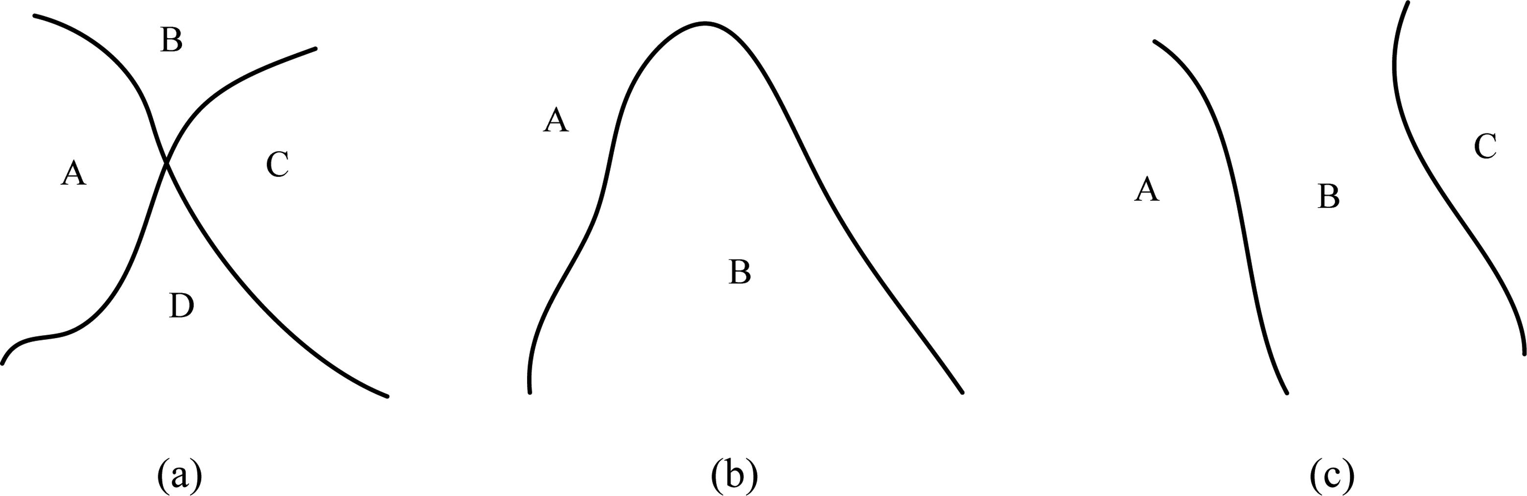
Task space and neighboring singularities. (a) Case 1. (b) Case 2. (c) Case 3.

Position-singularity-free path planning in the moving plane

Existence identification of position-singularity-free path

The coordinates of the task points P_i and P_f in the moving frame V-xy as shown in Figure 4 are denoted as P _i (x_i , y_i ) and P _f (x_f , y_f ), respectively. The simultaneous equations consisting of line P_iP_f and position-singularity curve can be constructed as

$y=\frac{y_f-y_i}{x_f-x_i}(x-x_i)+y_i$

4

$a{x}^2+2bxy+2dx+2ey+f=0$

5

Figure 4.

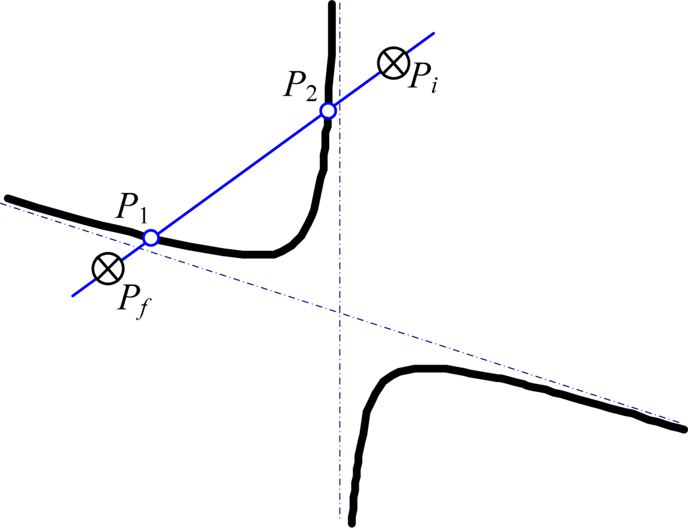
Case of hyperbola. (a) One case. (b) The other case.

Two real solutions of equations (4) and (5) are denoted as P ₁(x ₁, y ₁) and P ₂ (x ₂, y ₂), where only one solution can be regarded as two same solutions. The two real solutions are also the coordinates of the intersecting points of the line P_iP_f and the singularity locus in the moving plane. It is pointed out that the position-singularity locus represented as shown in equation (5) may be a set of hyperbolas, four pairs of intersecting lines, a parabola, two parallel lines, or one line all of which parallel to the ridgeline, that is, y-axis of the moving coordinates V-xy. ²⁶ The geometric properties determined by both values of δ and Δ, where

$\mathit{\delta }=-b^2\le 0,\Delta =-a{e}^2-b^{2}f+2bde$

When det( J _i ) × det( J _f ) > 0, whether a singularity-free path exists between the task points P_i and P_f can be known according to the following cases:

(1) When δ = 0 and Δ ≠ 0, equation (5) represents a parabola. If both of the task points locate at the same zone divided by the position-singularity locus as shown in Figure 6, a singularity-free path connecting P_i and P_f exists.

(2) If and only if (φ, ψ) = (±90°,=±90°), then δ = 0 and Δ = 0. Equation (5) designates into two parallel lines or one line, all of which parallel to the y-axis of the V-xy coordinates systems. If

$\begin{array}{l}\text{min}\left(x_1,x_2\right)<x_i,x_f<\text{max}\left(x_1,x_2\right),\\ \text{or}\hspace{0.17em}{x}_1,x_2<x_i,x_f,\\ \text{or}\hspace{0.17em}{x}_i,x_f<x_1,x_2,\end{array}$

a singularity-free path connecting P_i and P_f is permitted, which is shown in Figure 5.

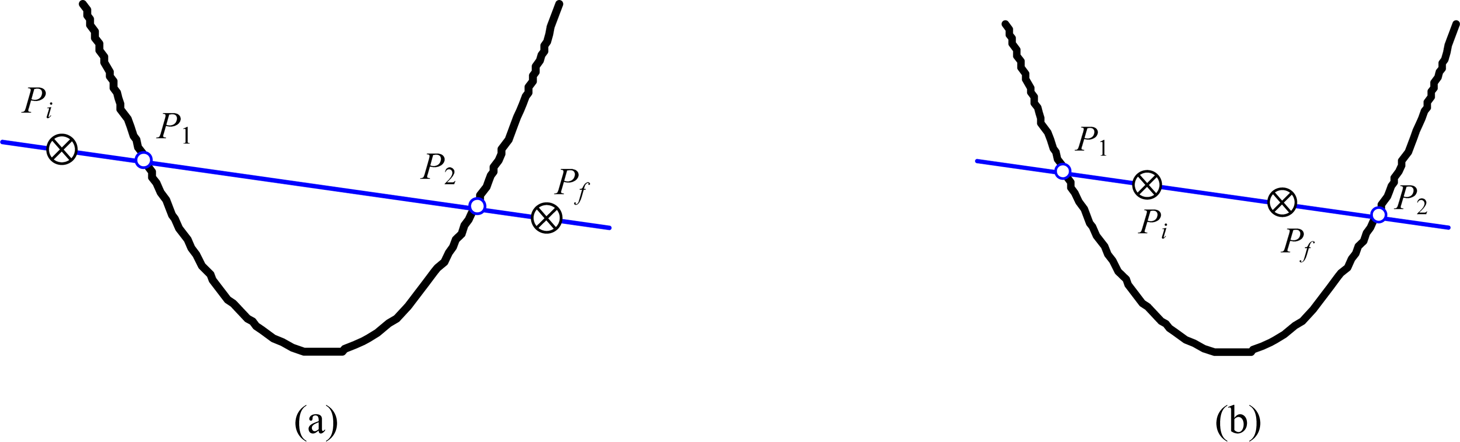
• (3) When δ < 0, equation (4b) describes a set of hyperbolas or a pair of intersecting lines.

• If x ₁, x ₂ ∉ ℜ, line P_iP_f does not intersect the singularity locus, thus P_i and P_f can also be connected by a singularity-free path as shown in Figure 7.

• If min(x_i , x_f ) < x ₁, x ₂ < max(x_i , x_f ) and (x ₁ + e/b) × (x ₂ + e/b) > 0, P_i and P_f locate on the same side of line x = −e/b. Figure 8 reveals that a singularity-free path connecting P_i and P_f is permitted.

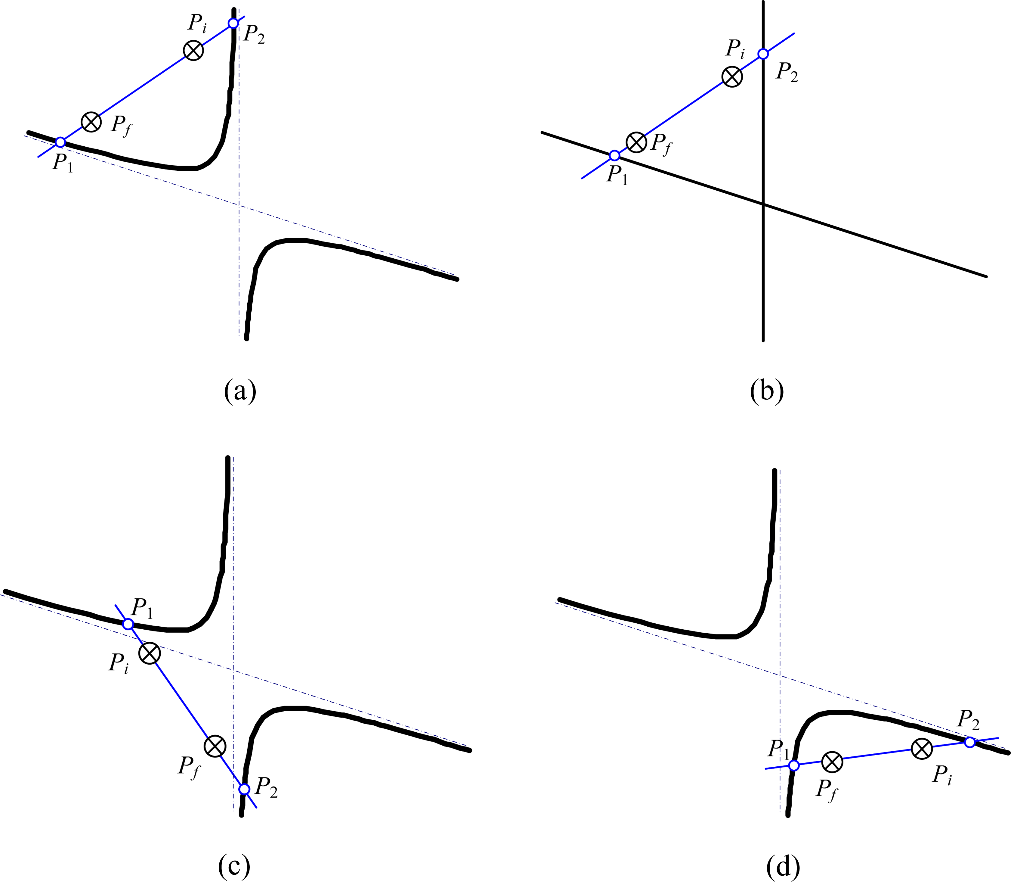
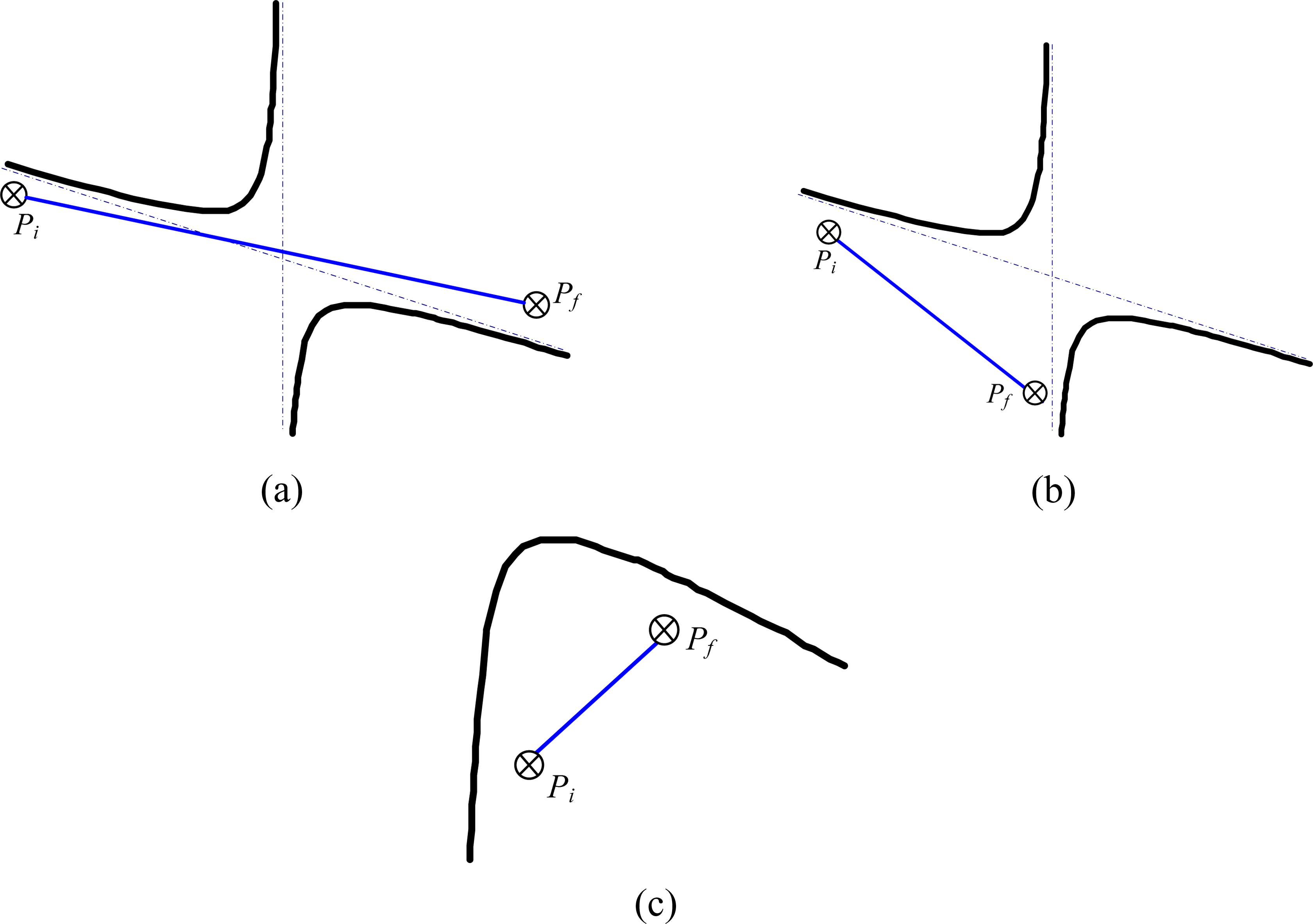
• If min(x_i, x_f ) < x ₁, x ₂ < max(x_i , x_f ) and (x ₁ + e/b) × (x ₂ + e/b) ≤ 0, then singularity-free path connecting P_i and P_f is absent. As shown in Figure 9(a), when (x ₁ + e/b) × (x ₂ + e/b) < 0, P_i and P_f are on the different sides of asymptotic line x = −e/b. As shown in Figure 9(b), when (x ₁ + e/b) × (x ₂ + e/b) = 0, one of P_i and P_f is in line x = −e/b.

Figure 5.

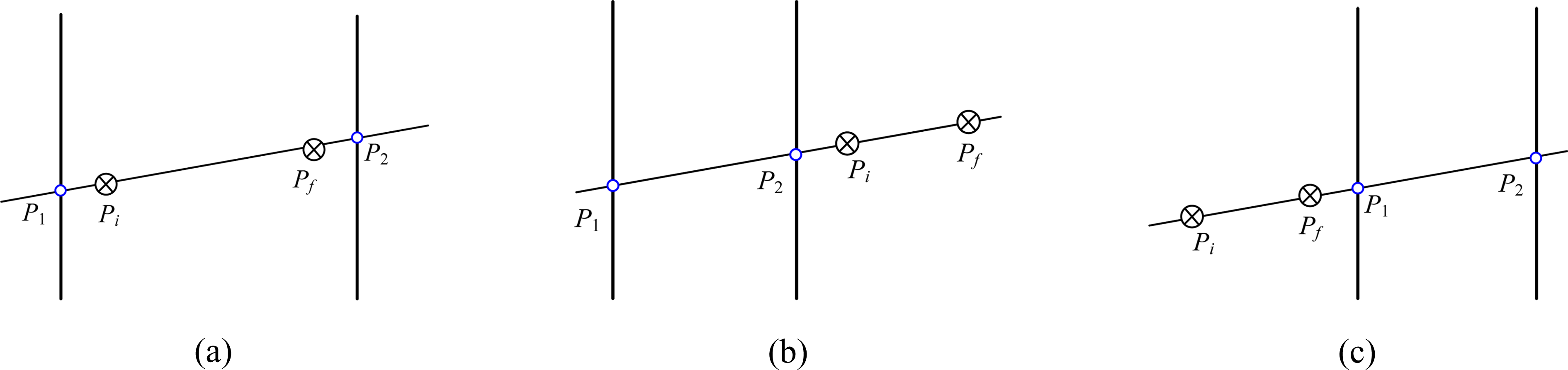
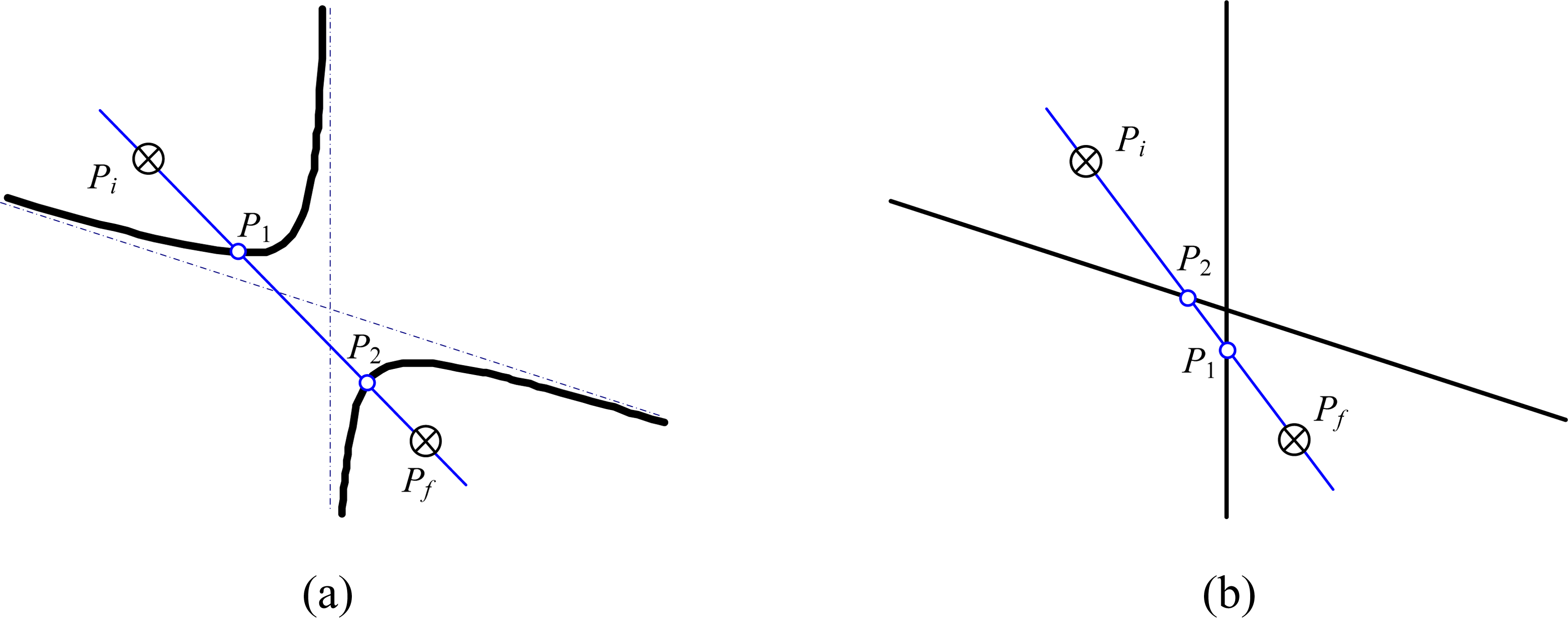
Case of parallel lines. (a) min(x ₁, x ₂) < x_i , x_f < max(x ₁, x ₂). (b) x ₁, x ₂ < x_i , x_f , (c) x_i , x_f < x ₁, x ₂.

Figure 6.

Case of min(x_i , x_f ) < x ₁, x ₂ < max(x_i , x_f ). (a) Case 1. (b) Case 2. (c) Case 3. (d) Case 4.

Figure 7.

Case of x ₁, x ₂ ∉ ℜ.

Figure 8.

Case of min(x_i , x_f ) < x ₁, x ₂ < max(x_i , x_f ) and (x ₁ + e/b) × (x ₂ + e/b)>0.

Figure 9.

Case of min(x_i , x_f ) < x ₁, x ₂ <max(x_i , x_f ). (a) (x ₁ + e/b) × (x ₂ + e/b) < 0. (b) (x ₁ + e/b) × (x ₂ + e/b) = 0.

From the abovementioned discussion, whether a singularity-free path exists between the task points P_i and P_f locating in the moving plane can be identified in Figure 10.

Figure 10.

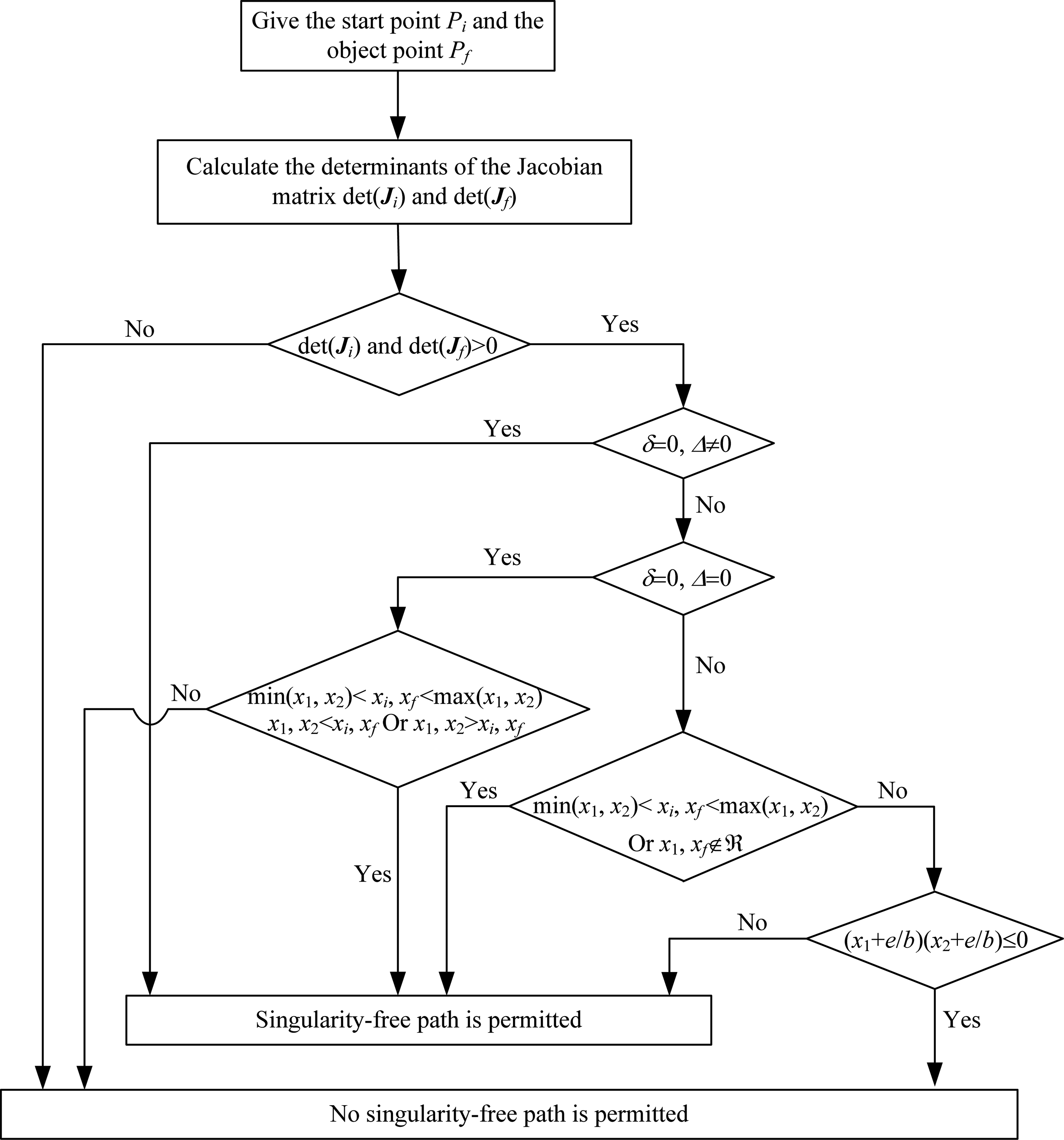
Existence identification of position singularity-free path.

Method of position-singularity-free path planning

If P_i and P_f can be connected by a singularity-free path, whose existence can be identified in Figure 10, and

$\begin{array}{l}{x}_1,x_2<x_i,x_f\hspace{0.17em}\text{or}\hspace{0.17em}\hspace{0.17em}{x}_i,x_f<x_1,x_2\hfill \\ \text{or min}\left(x_1,x_2\right)<x_i,\hspace{0.17em}{x}_f<\text{max}\left(x_1,x_2\right)\hfill \\ \text{or }\left(x_1,x_2\right)\hspace{0.17em}\notin \hspace{0.17em}{\Re }^2\hfill \end{array}$

6

the relative positions of P_i and P_f can be represented as one case in Figure 11(a) to (c), the straight line P_iP_f connecting P_i and P_f is singularity-free. If the coordinates of P_i and P_f do not satisfy equation (6), the singularity-free path should be planned as a curve to avoid the singularity locus, which is shown in Figure 12.

Figure 11.

Straight singularity-free path. (a) Type 1. (b) Type 2. (c) Type 3.

Figure 12.

Curvilinear singularity-free path.

In Figure 12, (x _0i , y _0i ) are the discrete points of line P_iP_f . (x_si , y_si ) is the intersecting point of the singularity locus and the line, which parallels the y-axis and passes through point (x _0i , y _0i ). According to the geometrical property of the position-singularity locus in the moving plane, the position-singularity locus written as a function y in terms of x is convex or concave. Thus, (x_si , y_si ) can be derived as

$\begin{array}{l}{x}_{pi}=x_{si}+\text{sign}\left(\frac{\text{d}y}{\text{d}x}\right)\Delta x\\ y_{pi}=y_{si}-\text{sign}\left(\frac{d^{2}y}{d{x}^2}\right)\Delta y\end{array}$

7

where, sign(·) is determined by the following

$\begin{array}{l}\text{If }(\cdot )>0,\text{ sign}(\cdot )=1\\ \text{If }(\cdot )<0,\text{ sign}(\cdot )=-1\\ \text{If }(\cdot )=0,\text{ sign}(\cdot )=0\end{array}$

Values of Δx and Δy are determined by the requisite accuracy of the planned path. dy/dx and d² y/dx ² can be obtained according to the following equation

$y=-\frac{1}{2}\frac{a{x}^2+2dx+f}{bx+e}$

8

They can be concluded as

$\frac{\text{d}y}{\text{d}x}=-\frac{1}{2}\frac{2ax+2d}{bx+e}+\frac{1}{2}\frac{(a{x}^2+2dx+f)b}{{(bx+e)}^2}$

$\frac{{\text{d}}^{2}y}{\text{d}{x}^2}=-\frac{a}{bx+e}+\frac{(2ax+2d)b}{{(bx+e)}^2}-\frac{(a{x}^2+2dx+f)b^2}{{(bx+e)}^3}$

After connecting P_i , (x_pi , y_pi ), and P_f successively, the singularity-free path from point P_i to point P_f represented in the moving frame V-xy can be obtained.

The above mentioned singularity-free path planning only considers the case of θ ≠ 0. If θ = 0, it can be divided into the following three cases:

Case 1. If Z = 0, namely the moving platform and the fixed one coincide, the mechanism is in singularity.

Case 2. If Z ≠ 0 and (φ + ψ) = ±90°, the mechanism is in singularity.

Case 3. If Z ≠ 0 and (φ + ψ) ≠ ±90°, any path connecting P_i and P_f is singularity-free.

Numerical examples

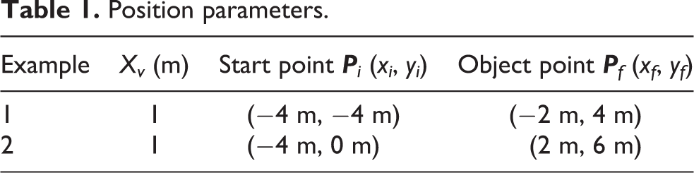
Geometrical parameters of the mechanism are given as follows: R _m = 1, R _b = 2, β _m = 75°, and β _b = 105° without considering the structural constraints. The orientation parameters are represented by standard ZYZ-Euler parameters and given as (φ, θ, ψ) = (60°, 30°, −45°). The position parameters of the task points P_i and P_f are given as shown in Table 1.

Table 1.

Position parameters.

Example	Xv (m)	Start point P i (xi , yi )	Object point P f (xf , yf )
1	1	(−4 m, −4 m)	(−2 m, 4 m)
2	1	(−4 m, 0 m)	(2 m, 6 m)

When the PM works near the singular configuration, the Jacobian matrix of the mechanism is ill-conditioned and the performance of the mechanism is poor. The condition number of the Jacobian matrix is an important performance index and can be used to estimate whether the mechanism is singular. Therefore, the condition number of the Jacobian matrix is applied to verify the method of the singularity-free path planning.

As shown in Figure 10, the determinants of the Jacobian matrices of the mechanism corresponding to the task points should be computed in advance as shown in Table 2.

Table 2.

Determinants of the Jacobian matrices corresponding to the task points.

Example	Xv (m)	det( J i ) corresponding to (xi , yi )	det( J f ) corresponding to (xf , yf )
1	1	149.643290188519	−66.2713396427308
2	1	27.912443480646	55.1412110112912

For example 1, according to Figure 10, as det( J _i ) × det( J _f ) < 0, no singularity-free path from point P_i to point P_f is permitted. The positions of the task points as shown in example 1 in the moving plane represented in V-xy frame are described in Figure 13. It can be shown that no singularity-free path connecting the two task points is permitted.

Figure 13.

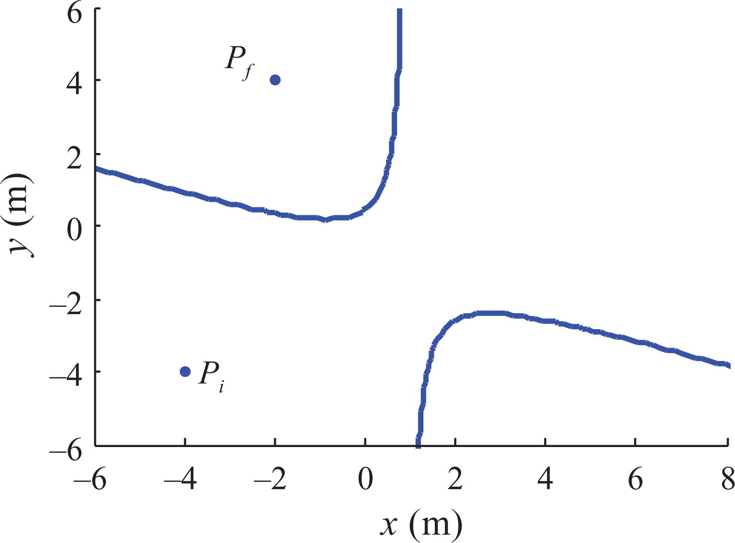
Task points in example 1.

For example 2, as det( J _i ) × det( J _f ) > 0, whether the singularity-free path exists can be identified using Figure 10. It can be obtained that δ = −603.43448 and Δ = −34165.75597. Solving equations (4) and (5) yields the intersection point of line P_iP_f between singularity locus in the moving frame V-xy as

$\begin{array}{l}\left(x_1,y_1\right)=\left(0.75673 \text{m},4.75673 \text{m}\right)\hfill \\ \left(x_2,y_2\right)=\left(-3.29892 \text{m},0.70108 \text{m}\right)\hfill \end{array}$

It can be shown that (x ₁, y ₁) ≠ (x ₂, y ₂), which does not satisfy min(x ₁, x ₂) < x_i , x_f < max(x ₁, x ₂). Besides, it can be concluded that −e/b = −0.955478 and (x ₁ + e/b) × (x ₂ + e/b)>0. Therefore, according to Figure 10, the task points can be connected by a singularity-free path, which can be obtained by the method described in Figure 12 and equation (7). Otherwise, if the two task points are connected by line P_iP_f as shown in Figure 14, the path must pass through the singularity locus. The condition numbers corresponding to the line path in discretization are shown in Figure 15.

Figure 14.

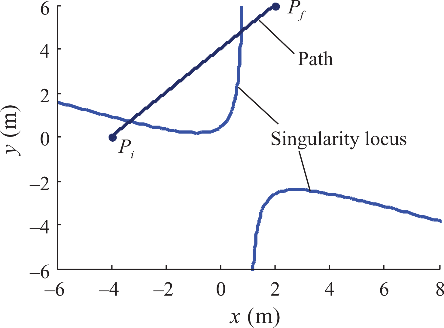
Line path of example 2.

Figure 15.

Condition number of the line path.

A singularity-free path obtained by the method described in Figure 12 and equation (7) is shown in Figure 16. The condition number for the singularity-free path is represented in Figure 17, where Δx = Δy = 0.5 m. It can be shown that the path descried in Figure 16 can avoid the singularity using the method of singularity-free path planning.

Figure 16.

Singularity-free path of example 2.

Figure 17.

Condition number for the singularity-free path.

It should be pointed out that the condition number of the singularity-free path is still large because it can also be influenced by other parameters including orientation parameters (θ, φ, ψ) and position parameter of the moving plane X_v . However, the condition number of the singularity-free path changes slowly and does not change suddenly to extremely large when the mechanism is singular. Therefore, the method of the position-singularity-free path planning proposed here is effective, which is the main purpose of this section.

Orientation-singularity-free path

Orientation transformation of a rigid body

The unit quaternion can describe an orientation transformation and can be written as the trigonometric form and the exponential product form

$\mathit{Q}=\text{cos}\frac{\mathit{\theta }}{2}+\xi \text{sin}\frac{\mathit{\theta }}{2}=\text{exp}\left(\xi \frac{\mathit{\theta }}{2}\right)$

9

$\Delta Q(t)=\text{exp}\left(\frac{1}{2}\omega (t+\epsilon \Delta t)\Delta t\right)$

10

where ∊ ∈ [0,1], ω (t + εΔt) is the angular velocity in the range [t, t + Δt] and regarded as a constant value. The definition of the unit quaternion and the orientation representation of the rigid body by using the unit quaternion as the orientation parameters are given in Appendix 1. Consider Δt tends to zero, the accurate increment quaternion can be written as

$\text{d}Q\text{(}t\text{)}=\text{exp}\left(\frac{1}{2}\omega \text{(}t\text{)d}t\right)$

11

Divide [0, T] equally by the interval

$\Delta t_i=t_{i+1}-t_i,\hspace{0.17em}\text{max}\left|\Delta t_i\right|\le \frac{kT}{N} (i=1,2,\dots ,N-1;i+1=2,3,\dots ,N)$

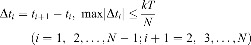
The relation between Q _{i +1} and Q _i can be derived as

$\begin{array}{l}Q(t_{i+1})=\Delta Q(t_i)\circ Q(t_i)\\ \hspace{0.17em}\hspace{0.17em}=\text{exp}\left(\frac{1}{2}\omega (t_i+{\epsilon }_{i+1}\Delta t_{i+1})\hspace{0.17em}\Delta t_{i+1}\right)\circ Q(t_i){\epsilon }_i\in [0,1]\end{array}$

12

where Q _{i +1} and Q _i are the orientation representations of the rigid body at t_{i +1} and t_i , Δ Q _i is the orientation transformation from Q _i to Q _{i +1}. Set Q ₀ as the initial orientation of the rigid body, equation (12) can be written as

$\begin{array}{l}Q(t_{i+1})=\Delta Q(t_i)\circ Q(t_i)\\ \hspace{0.17em}\hspace{0.17em}\hspace{0.17em}\hspace{0.17em}=\text{exp}\left(\frac{1}{2}\omega (t_i+{\epsilon }_{i+1}\Delta t_{i+1})\hspace{0.17em}\Delta t_{i+1}\right)\circ \cdots \circ \text{exp}\left(\frac{1}{2}\omega (t_1+{\epsilon }_2\Delta t_2)\hspace{0.17em}\Delta t_2\right)\circ \text{exp}\left(\frac{1}{2}\omega ({\epsilon }_1\Delta t_1)\hspace{0.17em}\Delta t_1\right)\circ Q_0\\ \hspace{0.17em}\hspace{0.17em}\hspace{0.17em}\hspace{0.17em}=\text{exp}\left({\xi }_{i+1}\frac{\Delta {\mathit{\theta }}_{i+1}}{2}\right)\circ \cdots \circ \text{exp}\left({\xi }_2\frac{\Delta {\mathit{\theta }}_2}{2}\right)\circ \text{exp}\left({\xi }_1\frac{\Delta {\mathit{\theta }}_1}{2}\right)\circ Q_0\hspace{0.17em}\end{array}$

13

and can be graphically represented as shown in Figure 18.

Figure 18.

Orientation kinematics equation of the rigid body using the spherical representation.

Time optimal orientation path of a rigid body

Both of an orientation transformation M or an orientation transformation Σ ∘ P can represent that the rigid body rotates from orientation Λ to orientation N , which is shown in Figure 19 using the spherical representation of the unit quaternion. Rotor angle of Σ ∘ P is longer than rotor angle of M . Therefore, orientation transformation M is the shortest orientation path, also called time optimal orientation path. There is

$\mathit{N}=\mathit{M}\circ \Lambda$

14

M can be derived according to the following expression

$\mathit{M}=\mathit{N}\circ {\Lambda }^{-1}$

15

Write M as the trigonometric form

$M=({\mathit{\mu }}_0,\mathit{\mu })=\text{cos}\frac{\phi }{2}+\mu \text{sin}\frac{\phi }{2}$

16

The time optimal orientation path form Λ to N with respect to the fixed frame can be obtained as

$\mathit{Q}\left(t\right)=\mathit{M}\left(t\right)\circ \Lambda$

17

where

$M(t)=\text{cos}{\displaystyle {\int }_{\text{0}}^t\frac{\mathit{\omega }(t)}{2}\text{d}t}+\mu \text{sin}{\displaystyle {\int }_{\text{0}}^t\frac{\mathit{\omega }(t)}{2}\text{d}t},\varphi ={\displaystyle {\int }_{\text{0}}^t\frac{\mathit{\omega }(t)}{2}\text{d}t}$

and ω(t) is the angular velocity at the moment of t.

Figure 19.

Time optimal orientation motion of the rigid body using the spherical representation.

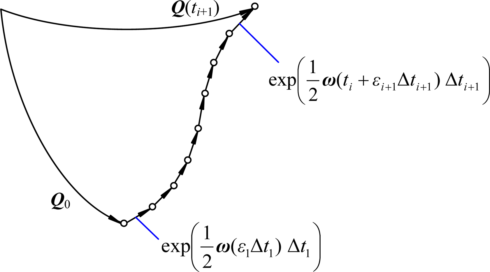
After dividing the time range [0, T] equally by N + 1 intervals, in which every angular velocity is considered as constant ω(t), the time optimal orientation path written as equation (18) which can be discretized as

$\mathit{Q}\left(t_{i+1}\right)=\mathit{M}\left(t_{i+1}\right)\circ \mathit{M}\left(t_i\right)\circ \cdots \circ \mathit{M}\left(t_1\right)\circ \Lambda$

18

where

$M(t_{i+1})=\text{cos}\left(\frac{1}{2}{\displaystyle \sum _{k=0}^i\mathit{\omega }}(t_i+{\epsilon }_i\Delta t)\Delta t_i\right)+\mathit{\mu }\text{sin}\left(\frac{1}{2}{\displaystyle \sum _{k=0}^i\mathit{\omega }}(t_i+{\epsilon }_i\Delta t)\Delta t_i\right)\left(i=0,1,2,\dots ,N\right)$

19

where t ₀ = 0, ∊_i ∈ [0, 1]. The time optimal orientation path described as equation (20) can also be written as the exponential product form

$\begin{array}{l}Q(t_{i+1})=\text{exp}\left(\frac{1}{2}\omega (t_i+{\epsilon }_{i+1}\Delta t_{i+1})\hspace{0.17em}\Delta t_{i+1}\right)\circ \cdots \circ \text{exp}\left(\frac{1}{2}\omega (t_1+{\epsilon }_2\Delta t_2)\hspace{0.17em}\Delta t_2\right)\circ \text{exp}\left(\frac{1}{2}\omega ({\epsilon }_1\Delta t_1)\hspace{0.17em}\Delta t_1\right)\circ \Lambda \\ \hspace{0.17em}\hspace{0.17em}\hspace{0.17em}\hspace{0.17em}=\text{exp}\left(\mu \frac{\Delta {\mathit{\theta }}_{i+1}}{2}\right)\circ \cdots \circ \text{exp}\left(\mu \frac{\Delta {\mathit{\theta }}_2}{2}\right)\circ \text{exp}\left(\mu \frac{\Delta {\mathit{\theta }}_1}{2}\right)\circ Q_0\hspace{0.17em}.\end{array}$

20

where Q ₀ = Λ and is the start orientation with respect to the fixed frame. The orientation of the rigid body at time t_{i +1}, Q (t_{i +1}), can be graphically described using the spherical representation as shown in Figure 20.

Figure 20.

Discrete representation of the orientation path of the rigid body.

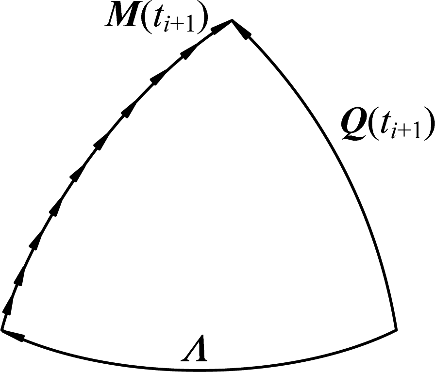
The unit quaternion, Q (t) = (q ₀(t), q ₁(t), q ₂(t), q ₃(t)), representing the orientation path of the rigid body rotates from start orientation, Λ = (λ ₀, λ ₁, λ ₂, λ ₃), to objective orientation, N = (ν ₀, ν ₁, ν ₂, ν ₃), can be obtained using equation (20). The vector representation of the unit quaternion (q ₁(t), q ₂(t), q ₃(t)), which has three independent variables, can be graphically described as a trajectory curve representing the optimal orientation path with starting point λ (λ ₁, λ ₂, λ ₃) and object point μ (μ ₁, μ ₂, μ ₃) in the 3-D Cartesian coordinate system. The orientation path is generally a curve except that one of the starting point λ and the finishing point μ locates at the origin of the coordinates, in which case the orientation path is a line from λ to μ in the Cartesian coordinate system.

Optimal orientation-singularity-free path planning of the mechanism

As the 3-D orientation transformation of the moving platform of the GSPM is also the rigid transformation in the SO(3), the optimal time orientation-singularity-free path planning is explored using the results of the optimal time orientation transformation of a rigid body and the distribution of the orientation-singularity for a given position and is detailed by a numerical example for ease of exposition in the following.

Structure parameters of the mechanism are given as shown in the section “Method of position-singularity-free path planning.” Here the starting orientation is given as Λ = (1, 0, 0, 0) and the object orientation is N = ( $\sqrt{10}/10$ , 0, −9/10, 3/10) for a given position. An orientation-singularity-free path can be planned using the aforementioned method as follows.

The unit quaternion for time optimal orientation transformation from Λ to N without considering the orientation-singularity locus for the given position (0, 0, 4) can be obtained as

$M=N\circ {\Lambda }^{-1}=(\sqrt{2}/2,\hspace{0.17em}0,\hspace{0.17em}-1/2,\hspace{0.17em}1/2)$

21

The rotated angle of moving platform of the mechanism is

$\mathit{\theta }=2\text{arccos}{\mathit{\mu }}_0=2\text{arccos}\hspace{0.17em}(\sqrt{2}/2)=\pi /2$

22

According to equation (20), the orientation path of the moving platform can be derived as

$Q\text{(}{t}_i)=\left[\text{cos}\hspace{0.17em}\left(i\cdot \frac{\Delta \mathit{\theta }}{2N}\right)+{\xi }_i\text{sin}\hspace{0.17em}\left(i\cdot \frac{\Delta \mathit{\theta }}{2N}\right)\right]\circ (1,\hspace{0.17em}0,\hspace{0.17em}0,\hspace{0.17em}0)\left(i=0,1,\dots ,N\right)$

where the unit direction vector ξ _i can be obtained using equation (9). Figure 21 shows the time optimal orientation path Q , where q ₁(t) = 0, without considering the orientation-singularity locus, and Figure 22 describes the condition number of the Jacobian matrix of the mechanism corresponding to the orientation path Q .

Figure 21.

Time optimal orientation path without considering the singularity.

Figure 22.

Condition number of the Jacobian matrix of the mechanism without considering the singularity.

According to Figures 21 and 22, it can be shown that the time optimal orientation path by directly using the advanced method in section “Orientation transformation of a rigid body” may pass through the singular configuration which must be avoided. After observing the orientation-singularity locus for the given position as shown in Figure 21, the time optimal orientation-singularity-free path can be obtained by setting an interim orientation point Q _mid = ( $\sqrt{2}/2$ , 0, −1/2, 1/2). Thus, the moving platform firstly rotates from Λ = (1, 0, 0, 0) to Q _mid = ( $\sqrt{2}/2$ , 0, −1/2, 1/2) and then to N = ( $\sqrt{10}/10$ , 0, −9/10, 3/10), where the two unit quaternions representing the two quick orientation transformations can be derived from equation (15) as

$M_1=Q_{mid}\circ {\Lambda }^{-1}=(\sqrt{\text{2}}/2\text{, 0,}-\text{1/2, 1/2})$

$M_2=N\circ Q_{mid}^{-1}=(\sqrt{20}/20,\hspace{0.17em}3/10,\hspace{0.17em}\sqrt{10}/20-9\sqrt{2}/20,\hspace{0.17em}3\sqrt{2}/20-\sqrt{10}/20)$

The rotation angles are

${\mathit{\theta }}_1=2\text{arccos}\hspace{0.17em}(\sqrt{2}/2)=\pi /2$

${\mathit{\theta }}_2=2\text{arccos}\hspace{0.17em}(\sqrt{20}/20)$

The time optimal orientation-singularity-free path can be easily obtained as

$Q_1=\left[\text{cos}\hspace{0.17em}\left(i\cdot \frac{\Delta {\mathit{\theta }}_1}{2N_{\text{1}}}\right)+{\mathit{\mu }}_1\text{sin}\hspace{0.17em}\left(i\cdot \frac{\Delta {\mathit{\theta }}_1}{2N_{\text{1}}}\right)\right]\circ (1,\hspace{0.17em}0,\hspace{0.17em}0,\hspace{0.17em}0)\left(i=0,1,\dots ,N_1\right)$

$Q_2=\left[\text{cos}\hspace{0.17em}\left(i\cdot \frac{\Delta {\mathit{\theta }}_2}{2N_{\text{2}}}\right)+{\mathit{\mu }}_1\text{sin}\hspace{0.17em}\left(i\cdot \frac{\Delta {\mathit{\theta }}_2}{2N_{\text{2}}}\right)\right]\circ (\sqrt{2}/2,\hspace{0.17em}0,\hspace{0.17em}-1/2,\hspace{0.17em}1/2)\left(i=0,1,\dots ,N_2\right)$

The replanned time optimal orientation-singularity-free path is shown in Figure 23, and the condition number of Jacobian matrix of the mechanism versus the orientation-singularity-free path is shown in Figure 24. It can be shown that the abovementioned method of orientation path planning can make an orientation transformation of the mechanism consuming minimum time without singularity.

Figure 23.

Time optimal orientation-singularity-free path.

Figure 24.

Condition number of the Jacobian matrix versus the orientation-singularity-free path.

Conclusion

1. For the investigation of position singularity-free path of the GSPM, based on the geometric property of position-singularity locus in the moving plane, whether a position-singularity-free path exists is addressed. After analyzing the coefficients characteristics of the singularity equation, the method of the path planning is developed. The method does not require careful observation of the singularity distributes. The research lays a foundation for our future work about the 3-D position-singularity-free path planning in a constant-orientation workspace.

2. The research of the position-singularity-free path of the GSPM in the moving plane has important value in practice. For example, the position-singularity-free path in the moving plane is essential to be planned, when the mechanism is applied on a sequential action, such as drilling holes, millings, or assembling in an oblique plane.

3. For the orientation singularity-free path of the GSPM, based on the quaternion algebra, after exploring the orientation kinematics of a rigid body and analyzing the orientation-singularity locus of the mechanism at a given position, the time optimal orientation singularity-free path planning of the mechanism, which can make the mechanism rotates quickly from an orientation to another with minimal time consumption and without singularity, is developed.

4. As the abovementioned orientation-singularity-free path depends much on the observation of distribution of the orientation singularity locus, this article explores the orientation-singularity-free path when one orientation parameter is set as constant value. The algorithm of automated search for a 3-D time optimal singularity-free path will be investigated in our future work.

5. The singularity-free path planning discussed in this article only considers the condition number of the Jacobian matrix which is a kinematics performance of the mechanism. Many factors can be used to measure the performance of the mechanism. Based on the discussion of this article, our future work will focus on the singularity-free path in the 6-D work space with some other optimal performance index, such as minimal time consumption, minimal energy consumption or relative small average driving force/torque.