Sage Journals: Discover world-class research

Abstract

The real-time calculations of the positioning error, error correction, and state analysis have always been a difficult challenge in the process of autonomous positioning. In order to solve this problem, a simple depth imaging equipment (Kinect) is used, and a particle filter based on three-frame subtraction to capture the end-effector’s motion is proposed in this article. Further, a back-propagation neural network is adopted to recognize targets. The point cloud library technology is used to collect the space coordinates of the end-effector and target. Finally, a three-dimensional mesh simplification algorithm based on the density analysis and average distance between points is proposed to carry out data compression. Accordingly, the target point cloud is fitted quickly. The experiments conducted in the article demonstrate that the proposed algorithm can detect and track the end-effector in real time. The recognition rate of 99% is achieved for a cylindrical object. The geometric center of all particles is regarded as the end-effector’s center. Furthermore, the gradual convergence of the end-effector center to the target centroid shows that the autonomous positioning is successful. Compared to traditional algorithms, both moving the end-effector and a stationary object can be extracted from image frames using a thesis. The thesis presents a simple and convenient positioning method, which adjusts the motion of the manipulator according to the error between the end-effector’s center and target centroid. The computational complexity is reduced and the camera calibration is eliminated.

Keywords

Autonomous positioning particle filter manipulator BP neural network point cloud library

Introduction

In computer vision, 3-D reconstruction refers to the process of 3-D scene restoration based on single view or multiple view images. There are four kinds of reconstruction methods: binocular stereo vision, sequential imaging, photometric stereo, and motion view analysis. The binocular stereo method is suitable for larger objects. The sequential imaging method is suitable for small objects. The photometric stereo and motion view analysis methods are suitable for large and complex scene reconstruction. Because single video information is incomplete, reconstruction based on it needs to use empirical knowledge. Multi-view reconstruction is relatively easy. It involves the calculation of the pose relation between the image coordinate frame and the world coordinate frame. Then, 3-D information is reconstructed using the plurality of 2-D images. But the computational complexity and cost is usually high. For 3-D reconstruction using simple depth image apparatus, there are a few studies showing certain results. Izadi et al.¹ propose a new 3-D reconstruction technology based on Microsoft Kinect. However, due to the limitation of the time of flight (TOF) technology, the accuracy of surface texture information is not high. The purpose of 3-D reconstruction is to provide the real-time monitoring of the end-effector positioning process and error. At the same time, it can lay a foundation for the debugging and analysis of the manipulator autonomy job task. Ma et al.² propose a gradual human reconstruction method based on individual Kinect. Body feature points are positioned in depth video frames combined with feature point detection and an error correction processing algorithm. The human body model is obtained by estimating the body size. Guo and Gao³ propose a robust automatic unmanned aerial vehicle (UAV) image reconstruction method using a batch framework. Li et al.⁴ find a multi-view reconstruction method from the perspective of motion visual analysis. A sparse point cloud and initial mesh are built using each view bias model. Lv et al.⁵ propose a Bayesian network model that describes body joint spatial relationships and dynamic characteristics. A golf swing process 3-D reconstruction system is built based on the similarities of swing movements. The problem of limb occlusion is effectively solved using an easy depth imaging device to capture motions. Lin et al.⁶ utilize an adaptive window stereo matching reconstruction method based on the integral gray variance and integral gradient variance. The image texture quality is determined according to the integral variance size. Related calculations are performed if the variance is greater than a preset threshold. The method needs to traverse the whole image to obtain the dense disparity map. Izadi et al.⁷ gather point cloud data using a single mobile and four fixed Kinect devices. The point cloud alignment and fitting problems are solved using iterative closest points. Kahl and Hartley⁸ convert 3-D reconstruction into a norm minimization problem. A closure approximate solution is derived using second-order cone programming. In the case of known camera rotation, the problem can be solved simultaneously for the shift and space position of the camera. Carbone and Gomez-Bravo⁹ introduce a method for the vision-based motion control of robot manipulators. A dynamic look-and-move system architecture is discussed, as a robot-vision system, which is closed at the task level. Kanatani et al.¹⁰ describe techniques for 3-D reconstruction from multiple images and summarize mathematical theories of statistical error analysis for general geometric estimation problems. Gruen and Thomas¹¹ address the question of where and how an imaged object is located in the object space. Basic component algorithms, such as image matching, segmentation, feature extraction, and so on, are favorably supported and constrained by the use of orientation parameters.

In this article, the target object is determined using back-propagation (BP) neural network recognition. The end-effector is extracted using motion state estimation based on a particle filter (PF). Then, the target centroid (TC) and end-effector center (EEC) are extracted. The spatial coordinates of the EEC and TC are calculated using coordinate frame transforming. The errors between EEC and TC are obtained. The error is mapped to the joint angle by inverse kinematics modeling. Then, the motion of the manipulator is adjusted using forward kinematics modeling. Therefore, autonomous positioning is achieved. The general flowchart is shown in Figure 1. The algorithm effectiveness can be verified using fast surface fitting.

Figure 1.

General flowchart.

End-effector motion estimation

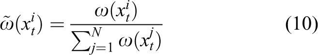
The position of the EEC can be obtained by motion estimation. The image coordinates of this center point can be transformed into the space coordinates according to hand-eye calibration. Then, an inverse kinematics model is used to transform the space coordinates of the center point into the joint angles. Accordingly, the end-effector is controlled to reach the target position.

The moving object and static background are separated from frame-stream images using the three-frame differencing method proposed by Martin and Robert.¹² The consecutive three-frame differencing method can better deal with the environmental noise, such as the weather, light, shadows, and messy background interference. It is shown to be better than the two-adjacent differencing method in double-shadow treatment proposed by Andre et al.¹³ The expressions are as follows

{\begin{matrix} d_{i, i - 1} (x, y) = | I_{i} (x, y) - I_{i - 1} (x, y) | \\ d_{i + 1, i} (x, y) = | I_{i + 1} (x, y) - I_{i} (x, y) | \end{matrix}

where $I_{i - 1} (x, y)$ denotes the pixel distribution of the previous image, $I_{i} (x, y)$ denotes the pixel distribution of the current image, $I_{i + 1} (x, y)$ denotes the pixel distribution of the next image, and $d_{i, i - 1} (x, y)$ and $d_{i + 1, i} (x, y)$ denote difference images. The binary form of the differencing image is obtained by selecting an appropriate threshold

{\begin{matrix} b_{i, i - 1} (x, y) = {\begin{matrix} 1; if d_{i, i - 1} (x, y) \geq T \\ 0; if d_{i, i - 1} (x, y) < T \end{matrix} \\ b_{i + 1, i} (x, y) = {\begin{matrix} 1; if d_{i + 1, i} (x, y) \geq T \\ 0; if d_{i + 1, i} (x, y) < T \end{matrix} \end{matrix}

where $b_{i, i - 1} (x, y)$ denotes the binary image and T denotes the threshold manually set to divide the foreground and background. If the value is less than T, it is the background, otherwise, it is the foreground. The “and” operation is done on the binary image. The double shadow becomes a single shadow. Another binary image is obtained

B_{i} (x, y) = {\begin{matrix} 1; if b_{i, i - 1} (x, y) & b_{i + 1, i} (x, y) = 1 \\ 0; if b_{i, i - 1} (x, y) & b_{i + 1, i} (x, y) \neq 1 \end{matrix}

Then, the morphology erosion and the dilation are applied to the binary image to remove holes.

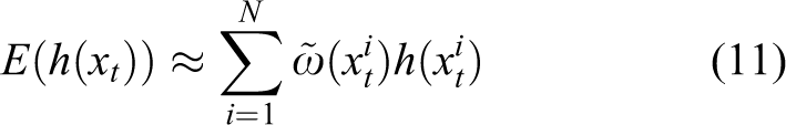
The motion state is estimated after the moving end-effector is extracted. So, it is convenient to calculate the position error between the end-effector and target object. The motion of the end-effector is nonlinear in video frames. The PF state estimation is adopted in the study by Suman et al.¹⁴ A series of random particle sets $S = {s (n), π (n) | n = 1, 2, \dots, M}$ with weights is used to approximate the posterior probability density function. s(n) denotes the sampling and it describes the prediction of the target state. π(n) denotes the discrete sampling probability. The PF is independent of the model of the system without linearization errors or Gaussian noise restrictions. It can be applied to any state and measurement model in any environment. The end-effector’s state equation and measurement equation are as follows

{\begin{array}{l} x_{t + 1} = F (x_{t}, N_{t}) \\ y_{t} = G (x_{t}, V_{t}) \end{array}

where x_t denotes the end-effector’s position state at time t, and y_0:t denotes the observation sequence {y₀,y₁,…,y_t} from the beginning time to the current time t. {y₀,y₁,…,y_t} corresponds to the position distribution sequence {x₀,x₁,…,x_t}. The state equation describes the state transition probability $p (x_{t + 1} | x_{t})$ . The function F is the target state function in the time domain. The measurement equation describes the conditional probability $p (y_{t} | x_{t})$ in the presence of measurement noise. G is a nonlinear measurement function. The independent dynamic vectors N_t and V_t denote random white noise sequences in the discrete time domain. N_t denotes the state noise. V_t denotes the measurement noise. The autonomous positioning system of the manipulator is nonlinear and non-Gaussian. Theoretically, when the number of particles N→∞, the Monte Carlo method can always be used to approximate any real probability distribution. In the case of a given measurement sequence y_0:t, the end-effector’s position x_t at the current time is estimated.

In addition, assume that the target state follows a Markov process, namely, the current state depends only on the previous state. When the conditional probability $p (x_{t} | y_{0 : t})$ is used to describe a given observation sequence y_0:t, the state transition probability of the end-effector $p (x_{t} | x_{0 : t - 1})$ can be expressed as $p (x_{t} | x_{t - 1})$ . When the measured values are independent of the state space, according to the Bayes rule, the conditional probability $p (x_{t} | y_{0 : t})$ is calculated as follows

p (x_{t} | y_{0 : t}) = \frac{p (y_{t}, y_{0 : t - 1} | x_{t}) p (x_{t})}{p (y_{t}, y_{0 : t - 1})} = \frac{p (y_{t} | y_{0 : t - 1}, x_{t}) p (y_{0 : t - 1} | x_{t}) p (x_{t})}{p (y_{t} | y_{0 : t - 1}) p (y_{0 : t - 1})} = \frac{p (y_{t} | y_{0 : t - 1}, x_{t}) p (x_{t} | y_{0 : t - 1}) p (y_{0 : t - 1}) p (x_{t})}{p (y_{t} | y_{0 : t - 1}) p (y_{0 : t - 1}) p (x_{t})} = \frac{p (y_{t} | x_{t}) p (x_{t} | y_{0 : t - 1})}{p (y_{t} | y_{0 : t - 1})}

where $p (y_{t} | x_{t})$ defines the system measurement noise model. The a priori probability distribution $p (x_{t} | y_{0 : t - 1})$ describes the state transition probability density and system knowledge model. At time t − 1, according to the conditional probability density $p (x_{t - 1} | y_{0 : t - 1})$ of the end-effector’s motion state, the following formula is derived using the Chapman–Kolmogorov equation

p (x_{t} | y_{0 : t - 1}) = \int p (x_{t} | x_{t - 1}) p (x_{t - 1} | y_{0 : t - 1}) d x_{t - 1}

In equation (5), $p (y_{t} | y_{0 : t - 1})$ denotes the measurement vector

p (y_{t} | y_{0 : t - 1}) = \int p (y_{t} | x_{t}) p (x_{t} | y_{0 : t - 1}) d x_{t}

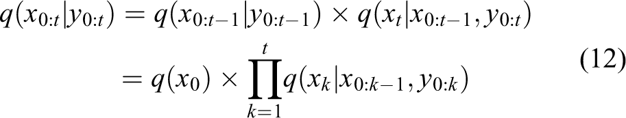
When the number of particle sets is large enough, these particles are set to replace the true posterior probability distribution. The end-effector’s posterior probability distribution $p (x_{t} | y_{0 : t})$ can be approximated by N independent identically distributed (IID) random variables

p (x_{t} | y_{0 : t}) \approx \frac{1}{N} \sum_{t = 1}^{N} δ (x_{t} - x_{t}^{i}) \equiv \hat{p} (x_{t} | y_{0 : t})

where $δ (x_{t} - x_{t}^{i})$ denotes the Dirac δ unit pulse function, and $x_{t}^{i}$ denotes IID of $p (x_{t} | y_{0 : t})$ . When N is large enough, $\hat{p} (x_{t} | y_{0 : t})$ can effectively approach the posterior distribution $p (x_{t} | y_{0 : t})$ . But, when $p (x_{t} | y_{0 : t})$ is a high-dimensional probability distribution, its direct sampling is very difficult. Usually, a proposal distribution $q (x_{t} | y_{0 : t})$ is selected to obtain a sample. Then, the nonlinear function h(x_t) of any state variable x_t can be estimated

E (h (x_{t})) = \int h (x_{t}) p (x_{t} | y_{0 : t}) d x_{t} = \int h (x_{t}) \frac{p (y_{0 : t} | x_{t}) p (x_{t})}{p (y_{0 : t}) q (x_{t} | y_{0 : t - 1})} q (x_{t} | y_{0 : t - 1}) d x_{t} = \frac{1}{p (y_{0 : t})} \int h (x_{t}) ω (x_{t}) q (x_{t} | y_{0 : t}) d x_{t}

where $ω (x_{t}) = \frac{p (y_{0 : t} | x_{t}) p (x_{t})}{q (x_{t} | y_{0 : t - 1})}$ denotes a nonnegative weight of sample $x_{t}^{i}$ . Normalization

\tilde{ω} (x_{t}^{i}) = \frac{ω (x_{t}^{i})}{\sum_{j = 1}^{N} ω (x_{t}^{j})}

So, $E (h (x_{t}))$ can be approximated as follows

E (h (x_{t})) \approx \sum_{i = 1}^{N} \tilde{ω} (x_{t}^{i}) h (x_{t}^{i})

When the sampling data $q (x_{0 : t - 1} | y_{0 : t - 1})$ at time t − 1 and the latest sample $q (x_{t} | x_{0 : t - 1}, y_{0 : t})$ at time t are known, the proposal distribution can be broken down into

\begin{array}{l} q (x_{0 : t} | y_{0 : t}) = q (x_{0 : t - 1} | y_{0 : t - 1}) \times q (x_{t} | x_{0 : t - 1}, y_{0 : t}) \\ = q (x_{0}) \times \prod_{k = 1}^{t} q (x_{k} | x_{0 : k - 1}, y_{0 : k}) \end{array}

The recursive calculation of weight $ω (x_{t}^{i})$

ω (x_{t}^{i}) = \frac{p (y_{0 : t} | x_{t}) p (x_{t})}{q (x_{t} | y_{0 : t - 1})} \propto \frac{p (x_{0 : t}^{i} | y_{0 : t})}{q (x_{0 : t}^{i} | y_{0 : t})} = \frac{p (y_{t} | x_{t}^{i}) p (x_{t}^{i} | x_{t - 1}^{i})}{q (x_{t}^{i} | x_{0 : t - 1}^{i}, y_{0 : t})} \times \frac{p (x_{0 : t - 1}^{i} | y_{0 : t - 1})}{q (x_{0 : t - 1}^{i} | y_{0 : t - 1})} = ω (x_{t - 1}^{i}) \times \frac{p (y_{t} | x_{t}^{i}) p (x_{t}^{i} | x_{t - 1}^{i})}{q (x_{t}^{i} | x_{0 : t - 1}^{i}, y_{0 : t})}

Object recognition

Image preprocessing

This section describes preprocessing based on Kinect RGB images. Target recognition is illustrated by an example using a cylindrical target object (CTO). The end-effector and CTO appear in the same video. First, image gray processing is carried out to convert color images to gray ones in order to reduce computation. The gray image gradation is 0–255. The grayscale method, Gray = 0.114B+0.587G+0.299R, is used, as in the study by Refael and Richard.¹⁵

Second, image median filtering is carried out. It is a type of nonlinear smoothing methods. Chang et al.¹⁶ find that it cannot blur edges while suppressing random noise. The gray values of pixels are sorted in a sliding window. The original gray value of each pixel in the window center is substituted by the median.

Third, mathematical morphology operations are carried out. Dilation and erosion operations are used in the study by Chang et al.¹⁷ They are widely used in edge detection, image segmentation, image thinning, noise filtering, and so on. Assume that E(x, y) denotes the binary image and B(s, t) denotes structural elements. The following operations are used.

Morphology dilation

X = E \oplus B = {(s, t) : B (s, t) \cap E \neq \emptyset}

Morphology erosion

Y = E ⊙ B = {(s, t) : B (s, t) \subset E}

Then, the weighted fusion between the input image and its “canny” operator detection is conducted. The threshold segmentation of the fusion image is carried out. Image segmentation is a basis for determining feature parameters. The whole contour of the object is obtained after image segmentation. An example is demonstrated in Figure 2. The shaded area represents the boundary. Finally, this should make the system possess capable of automatically extracting geometric features. These features should stay invariant when the image is transformed by translation, rotation, twisting, scaling, and so on.

Figure 2.

Calculation example of feature parameters.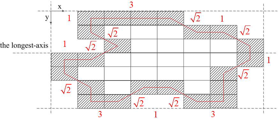

There are two kinds of CTO feature parameters: edge contour features and shape parameters. The parameters of contour points are edge contour features. Shape parameters include the perimeter, area, longest axis, azimuth, boundary matrix, and shape coefficient.

(I) Contour points represent the required number of pixels which can outline the contour. The number of contour points is 22 in Figure 2.

(II) The perimeter represents the contour length of the outer boundary. It can be calculated as the sum of the distances between two adjacent pixels on the outer boundary. Assume that the distance between two edge pixels sharing a side is 1, otherwise it is $\sqrt{2}$ . So, the perimeter is $14 + 8 \sqrt{2}$ in Figure 2.

(III) The area can be represented as the number of pixels in the target region. So, the area is 41 in Figure 2.

(IV) The longest axis denotes the maximum extension length of the target region, that is, the connection line of the maximum distance between two pixel points on the outer boundary. So, the longest axis is 8 in Figure 2.

(V) The azimuth represents the angle between the longest axis and the x-axis in the target region. So, the azimuth is 0 in Figure 2.

(VI) The boundary matrix denotes the minimum matrix encompassing the target region. It is also the intuitive expression of the flat level of the target region. It is composed of four outer boundary tangents. Two of them are parallel to the longest axis, and the other two are perpendicular to the longest axis. So, in Figure 2, the boundary matrix is

M = [\begin{array}{l} 0 & 1 & 1 & 1 & 1 & 0 & 0 & 0 \\ 0 & 1 & 0 & 0 & 0 & 1 & 1 & 0 \\ 0 & 0 & 1 & 0 & 0 & 0 & 0 & 1 \\ 1 & 1 & 0 & 0 & 0 & 0 & 0 & 1 \\ 1 & 0 & 0 & 0 & 0 & 0 & 1 & 0 \\ 0 & 1 & 0 & 1 & 1 & 0 & 1 & 0 \\ 0 & 1 & 1 & 0 & 0 & 1 & 1 & 0 \end{array}]

(VII) The shape coefficient denotes the ratio of the area to the square of the perimeter. So, the shape coefficient is 0.0639 in Figure 2.

Neural network recognition

This section describes recognition based on Kinect RGB images. A BP neural network learning algorithm is used in this article. This network can learn and store a large amount of input–output mappings. It is also a mathematical equation that does not use the description of these mappings in advance. Its learning rule is the gradient descent method. The mean square error (MSE) is minimized by adjusting the network weights and thresholds continuously. The network topology includes the input layer, the hidden layer, and the output layer.

Feature vectors are extracted as a training sample. The neural network is used as a classifier instead of the Euclidean distance method to implement target recognition.

The design of the input and output layers is as follows. The number of nodes is 7 in the input layer. The elements of the input vector are {contour points, perimeter, area, longest axis, azimuth, boundary matrix, and shape coefficients}. The number of nodes is 3 in the output layer. The elements of the output vector are {cylinder, square, and spherical}. The normalized values of the output are 0.1, 0.2 and 1, respectively. The design of the hidden layer is as follows: There are two hidden layers which include a logarithmic characteristic function and “purelin” function. The number of nodes is 20 in the first hidden layer. The number of nodes is 3 in the second hidden layer. A linear excitation function is used in the output layer. The number of hidden layers is related to the number of neurons and specific issues. At present, it is difficult to provide an accurate function to describe this relation. Experiments show that the accuracy of the network does not necessarily increase when the number of hidden layers and neurons is increased. The initial number of the hidden layers can be selected as

n' = \sqrt{m + n} + a

where m denotes the number of neurons in the input layer, n denotes the number of neurons in the output layer, and a denotes an integer from 1 to 10. Here, n′ is set to be 15.

The sample set is collected from a shooting scene of Kinect. In Figure 3, there are cylindrical objects, square objects, and spherical objects. There are 30 cylindrical objects (Figure 3(a)), 10 square objects (Figure 3(b)), and 10 spherical objects (Figure 3(c)). For each target object, there are 20 different viewing angles (the schematic diagram is shown in Figure 3(d) to (f)). So, the numbers of cylindrical objects, square objects, and spherical objects are 600, 200 and 200, respectively, in the sample set. In Figure 3(g), the edge contour is extracted. For the number of samples, there is no exact formula in any references. But, it is not the case where more is better. There are 970 samples in the study by Shi et al.¹⁸ and 150 samples in the study by Liu and You.¹⁹ In addition, Hao and Jiang²⁰ prove that the sample size 1000 seems reasonable according to the sample choice method.

Figure 3.

Image preprocessing. (a) 30 kinds of cylindrical objects. (b) 10 kinds of square objects. (c) 10 kinds of spherical objects. (d) RGB images and binary segmentation of cylindrical objects from different perspectives. (e) RGB images and binary segmentation of square objects from different perspectives. (f) RGB images and binary segmentation of spherical objects from different perspectives. (g) Edge contour extraction.

Network training: The weights of the neurons are adjusted in the training process. The training stops when the MSE reaches 10⁻⁷. The maximum number of iterations is set to 10,000. The momentum constant is set to 0.8. The initial learning rate is 0.01. The ratio of increase in the learning rate is 1.05. The decrease ratio of the learning rate is 0.7. The sample set is normalized. The range is [0,1]. The normalization function is

f (x) = \frac{1}{(1 + e^{- x})}

The TC is calculated after target identification. The shape of the target object is regular, so the spatial position of the TC is the destination of the end-effector positioning. The TC is calculated as follows

{\begin{cases} \bar{x} = \frac{\sum_{i_{b}}^{i_{e}} \sum_{j_{b}}^{j_{e}} i (p_{i j} - T)}{\sum_{i_{b}}^{i_{e}} \sum_{j_{b}}^{j_{e}} (p_{i j} - T)} \\ \bar{y} = \frac{\sum_{i_{b}}^{i_{e}} \sum_{j_{b}}^{j_{e}} j (p_{i j} - T)}{\sum_{i_{b}}^{i_{e}} \sum_{j_{b}}^{j_{e}} (p_{i j} - T)} \end{cases}

where i_b and i_e denote the minimum pixel and maximum pixel of the target object, respectively, along the row direction, j_b and j_e denote the minimum pixel and maximum pixel of the target object, respectively, along the column direction, T denotes the adaptive threshold, and p_ij denotes the grayscale value.

Autonomous positioning

Point cloud acquisition

The motion end-effector extracted from image frames belongs to the active object in the positioning system. Target objects identified from image frames belong to the passive object in the positioning system. After the active object and passive object are determined in the sections “End-effector Motion Estimation” and “Object Recognition,” their point cloud data (also called the target point cloud, TPC) is obtained by Kinect. It contains the 3-D coordinates and RGB information of each point.

The point cloud library (PCL) is an open-source point cloud processing library. It includes point cloud data acquisition and processing, filtering, feature extraction, surface reconstruction, point cloud registration, point cloud integration, and so on. The OpenNI is used as the system I/O interface in the PCL. Richard et al.²¹ suppose that the distance is d _raw from a point P to camera in the Kinect measurement space. According to the 3-D coordinate extraction method provided by Zhu et al.,²² the actual position of point P in the space is

d = K tan (H d_{raw} + L) - O

where d and d _raw are in centimeters, H = 3:5 × 10⁻⁴ rad, K = 12.36 cm, O = 3.7 cm, and L = 1.18 rad. Then, the coordinate (x, y, z)/cm is extracted as

{\begin{array}{l} x = (u - u_{0}) f_{x} d \\ y = (v - v_{0}) f_{y} d \\ z = d \end{array}

where (u, v) denotes the projection position of point P in the image frame

{\begin{matrix} f_{x} = 587.944 pixel, f_{y} = 589.418 pixel \\ u_{0} = 313.222 pixel, v_{0} = 259.304 pixel \end{matrix}

is the official calibration data. f_x and f_y denote the conversion factors between the imaging plane pixel and space physics length. u ₀ and v ₀ denote the image origin.

Point cloud processing

The number of the TPC is of order 10⁶ in each frame. The processing of huge and unordered data consumes a lot of time and hardware resources. It affects the speed of the algorithm. He et al.²³ find that noise in a point cloud can be removed by preprocessing based on density analysis. The point cloud distribution obtained from Kinect is not uniform. The average distance between each point and its neighborhood points follows approximately Gaussian distribution. There are some outliers in the point cloud data. Their neighborhood points are always closer. The neighborhood average distance (NAD) s is generally large. If the average distance is not in the standard range determined by the mean μ and standard deviation σ, the point is defined as an outlier, and it should be removed. The probability density function of the NAD is

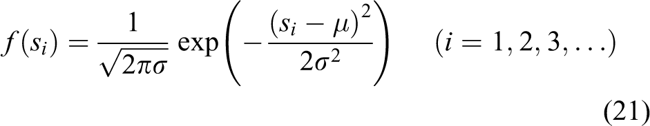
f (s_{i}) = \frac{1}{\sqrt{2 π σ}} exp (- \frac{{(s_{i} - μ)}^{2}}{2 σ^{2}}) (i = 1, 2, 3, \dots)

where s_i denotes the NAD of any point, μ denotes the mean of the NAD, and σ denotes the standard deviation. The number of neighborhood points is set to m. The multiple of the standard deviation is set to n. When the NAD of a point exceeds the global average distance nσ, the point should be marked as an outlier and removed. When m increases and n decreases, the noise determined to be outliers is lower. m and n are set to 25 and 4, respectively, by experiments.

TPC data compression

In order to achieve fast 3-D surface fitting, TPC data compression is necessary. Merry et al.²⁴ propose a 3-D mesh simplification algorithm based on the average distance between points. The 3-D mesh can be assumed to be a cube surrounded by the 3-D coordinates of the point set. The side length of the cube is the maximum coordinate difference between the 3-D data points. In the smallest mesh, the average distance method proposed selects a part of feature points instead of all data points. The accuracy of simplification is determined by the size of the mesh. When the cube mesh is smaller, the simplification precision is higher.

The idea of the average distance method is that when the point cloud density is higher, the distance between points is smaller. Otherwise, the size of the point cloud density can also be determined by the distance. According to the size of the point cloud density, the number of points to delete is chosen. The steps are as follows:

(I) Define the side length L of the cube mesh. Define the rate ξ between the expected simplification data and original data.

(II) Assume that a random point P is a starting point. The remaining point set is $P' = {{P'}_{i} (x_{i}, y_{i}, z_{i}), i = 1, 2, \dots, n}$ . Then, the distance d_i is calculated from P to any point of P ′.

(III) The average distance of P is

\bar{d} = \frac{\sum_{i = 0}^{n - 1} d_{i}}{n}

(IV) All point sets in the mesh are calculated according to the above steps. The points with the minimum average distance are simplified by ξ. Therefore, point cloud data compression is realized.

Coordinate frames transforming

In section “Point cloud acquisition,” the TPC extracted describes the positional relationship between the camera coordinate frame {c} and target coordinate frame {t}. However, this is not enough. According to the principle of inverse kinematics, the TPC needs to be transformed into the base coordinate frame. Thereby, the system can control the trajectory of the manipulator. The forward kinematics model describes the relative position of the end-effector coordinate frame {e} and base coordinate frame {b}. Now, the TPC is mapped to the spatial coordinates relative to {b}. The origin of the world coordinate frame {w} is set at the base. {b} and {w} coincide. Coordinate frame transforming is shown in Figure 4.

Figure 4.

Coordinate frame transforming.

The homogeneous transformation matrix describes the relative position of the two coordinate frames with dimension 4 × 4.

Definition: ^CT_B denotes the position of {c} in {b}, ^CT_E denotes the position of {c} in {e}, and ^ET_B denotes the position of {e} in {b}. Coordinate frame transforming is

{}^{C}T_{B} = {}^{C}T_{E} {}^{E}T_{B}

where ${}^{C}T_{E}$ can be calculated as in the study by Ivan et al.²⁵ Based on the forward kinematics model, ${}^{E}T_{B} = {}^{0}T_{N}$ . Therefore, the 3-D TPC is transformed into the base coordinate frame.

The spatial coordinates of the TPC are mapped to the rotation angles of each joint by inverse kinematics modeling.²⁶ The corresponding command is sent out to control the movement of the manipulator. The end-effector reaches the target position using forward kinematics. Therefore, autonomous positioning is achieved.

Finally, surface fitting is made as in the study by Bloomenthal²⁷ to validate the correctness of the proposed positioning method.

Experiment and analysis

The experimental platform consists of a computer (AcerTMP455, 16G memory, 500G SSD), manipulator system, and a simple depth imaging device Kinect, as shown in Figure 5. Kinect work principle specification is described on the corresponding webpage. The software includes VC++2010, OpenNI, MATLAB 2012a, and Kinect for Windows SDK v1.7.

Figure 5.

Experimental platform.

Kinematics analysis

The proposed method is illustrated using the example of a five-degree-of-freedom manipulator, as shown in Figure 6. There are five rotation axes, five joints, and three links. Five joints are the waist rotation joint (the first joint, J1), arm pitching joint (the second joint, J2), forearm pitching joint (the third joint, J3), wrist pitching joint (the fourth joint, J4), and wrist rotation joint (the fifth joint, J5). The DH parameters are determined as shown in Table 1, where θ_i denotes the rotation angle along the z-axis, α_i denotes the rotation angle along the x-axis, a_i denotes the distance along the x-axis between two neighbor z-axes, d_i denotes the distance along the z-axis between two neighbor x-axes, r₁ denotes the arm length, r₂ denotes the forearm length, and r₃ denotes the wrist length.

Figure 6.

Manipulator diagram.

Table 1.

DH parameters.

Links	θ_i (°)	α_i (°)	a_i (mm)	d_i (mm)
1	θ₁	0	67	0
2	θ₂	0	80	0
3	θ₃	0	r₁(490)	0
4	θ₄	0	r₂ (530)	0
5	θ₅	−90	0	r₃(480)

The transforming matrices are obtained as

{}^{0}T_{1} = [\begin{matrix} 1 & 0 & 0 & 0 \\ 0 & 1 & 0 & 0 \\ 0 & 0 & 1 & 0 \\ 0 & 0 & 0 & 1 \end{matrix}] {}^{1}T_{2} = [\begin{matrix} - 0.8940 & 0.4481 & 0 & 67 \\ 0 & 0 & - 1 & 0 \\ - 0.4481 & - 0.8940 & 0 & 0 \\ 0 & 0 & 0 & 1 \end{matrix}]

{}^{2}T_{3} = [\begin{matrix} - 0.5985 & - 0.8012 & 0 & 80 \\ 0.8012 & - 0.5985 & 0 & 0 \\ 0 & 0 & 1 & 0 \\ 0 & 0 & 0 & 1 \end{matrix}]

{}^{3}T_{4} = [\begin{matrix} - 0.4481 & - 0.8940 & 0 & 490 \\ 0 & 0 & - 1 & 0 \\ 0.8940 & - 0.4481 & 0 & 0 \\ 0 & 0 & 0 & 1 \end{matrix}] {}^{4}T_{5} = [\begin{matrix} 1 & 0 & 0 & 0 \\ 0 & 0 & 1 & 0 \\ 0 & - 1 & 0 & 0 \\ 0 & 0 & 0 & 1 \end{matrix}]

{}^{0}T_{5} = [\begin{matrix} - 0.4006 & 0.4481 & - 0.7992 & 433.5 \\ - 0.8940 & 0 & 0.4481 & 0 \\ 0.2008 & 0.8940 & 0.4006 & - 255.4 \\ 0 & 0 & 0 & 1 \end{matrix}]

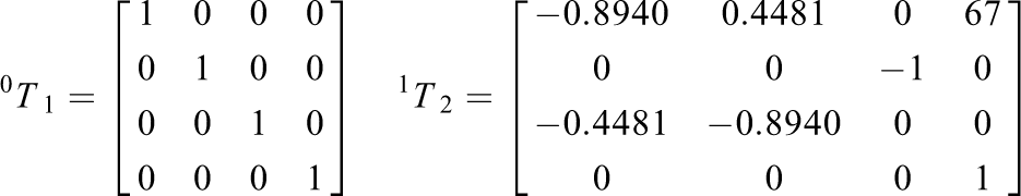
Because the origin of the base coordinate frame is set at the center of J1, and the waist length is 76 mm, the space motion range of J1 is (0, 0, 38 mm). The range of J2 is (0, 0, 76 mm). The space trajectory range of J3 is shown in Figure 7(a). The space trajectory range of J4 is shown in Figure7(b). The space trajectory range of the end-effector is shown in Figure 7(c).

Figure 7.

Joint motion trajectories. (a) Motion range of J3. (b) Motion range of J4. (c) Motion range of the end-effector.

Take point A (414 mm, 890 mm, 1045 mm) in the world coordinate frame as an example. The inverse kinematic solutions are shown in Table 2. The optimal solution (21.61, 125.73, 108.42, 99.41, 0) is obtained using the optimization method from the study by Hu and Li.²⁶

Table 2.

Inverse kinematic solutions.

Rotary angle (°) The number of solution (k)	θ₁	θ₂	θ₃	θ₄
1	21.61	83.82	91.38	160.23
2	21.61	87.63	87.98	147.20
3	21.61	91.44	87.00	138.17
4	21.61	95.25	87.15	130.92
5	21.61	99.06	88.07	124.79
6	21.61	102.87	89.59	119.47
7	21.61	106.68	91.63	114.82
8	21.61	110.49	94.14	110.75
9	21.61	114.30	97.09	107.19
10	21.61	118.11	100.46	104.13
11	21.61	121.92	104.24	101.53
12	21.61	125.73	108.42	99.41
13	21.61	129.54	112.98	97.74
14	21.61	133.35	117.90	96.53
15	21.61	137.16	123.17	95.78
16	21.61	140.97	128.77	95.49
17	21.61	144.78	134.67	95.67
18	21.61	148.59	140.84	96.31

End-effector state estimation

The video is transformed into the image frame format (480 × 640 × 3) as shown in Figure 8(a). There are 73 frames in total. The binary threshold T is set to 0.0118. The static background is extracted using the three-frame differencing method as shown in Figure 8(b). When the end-effector is moving, its moving area is extracted from each frame. It is marked with green squares as shown in Figure 8(c).

Figure 8.

Target Separation. (a) Image frame. (b) Static object extraction. (c) End-effector extraction.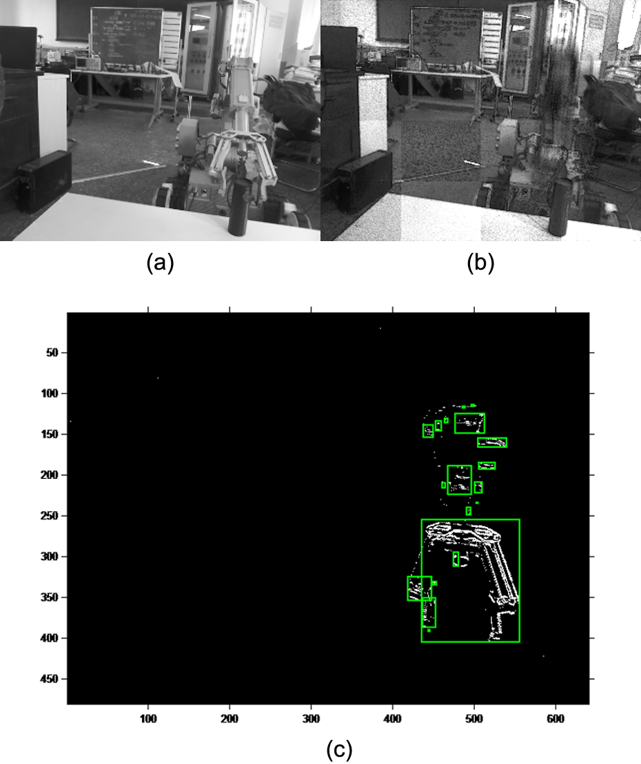

In the PF, the number of particles is M = 100. The process noise covariance is 10. The measurement noise covariance is 1. The initial state of the EEC and particles is shown in Figure 9(a). Red “·” denotes the EEC’s initial position. Black “·” denotes the distribution of 100 particles. Blue “·” denotes the geometric center of the particles.

Figure 9.

State estimation of end-effector. (a) Initial position of EEC, particles distribution, and initial position of particle center. (b) Motion of EEC is tracked by center of particles.

The tracking process of the end-effector using the PF is illustrated in Figure 9(b). Red “·” denotes the state change of the EEC. Black “·” denotes the state change of the particles. In the process of tracking, all particles are clustered. Blue “·” denotes the state change of the particle center. The clusters of the particles and their centers coincide substantially. During the end-effector moving, the center of the particles approaches the EEC gradually. Their centers almost coincide. The state trend is also almost the same. So, the EEC can be approximated using the geometric center of the particles. Therefore, the position of the end-effector can be obtained in real time.

The general trends of the actual position and estimated position coincide. This indicates that this algorithm can predict the end-effector’s position. At the same time, the experiment shows that the adaptability of the system is improved. While the static background is extracted, the moving end-effector is also detected and tracked in the scene.

Target recognition experiment

The edge contour of the target object is extracted according to the section “Object recognition.” Then, the shape parameters (seven kinds) are calculated to obtain the sample set. The dimension of the sample set is 1000 × 8 (cylindrical 600, square 200, and spherical 200). The dimension of the training set is 900 × 8 (cylindrical 540, square 180, and spherical 180). The dimension of the test set is 100 × 8 (cylindrical 60, square 20, and spherical 20). The normalization processing of the sample set is carried out. The situation with the BP network training is shown in Figure 10. This training takes 5 s with 47 iterations. The blue line represents the convergence of the training sample. The red line represents the convergence of the test sample. The network stops training when the MSE reaches 1.24 × 10⁻⁸. The test set converges when the MSE reaches 7.84 × 10⁻⁵. The function gradient decreases from 1.49 to 9.41 × 10⁻⁶. The dotted line denotes the preset MSE of the stopping training.

Figure 10.

Convergence of BP neural network training.

The results of the identification are shown in Figure 11. The horizontal axis denotes the number of test samples (per group). The vertical axis denotes the classification (identification result). Blue “.” denotes the network predictive result. Red “○” denotes the actual classification. If the classification is equal to 0.1, the target is a cylindrical object. If the classification is equal to 0.2, the target is a square object. If the classification is equal to 1, the target is a spherical object. From Figure 11, there is probably a one-to-one correspondence between the network classification and actual results. Fifty-nine cylindrical objects are identified correctly, one is identified to be square (probability 98.3%). Twenty square objects are all identified correctly (probability 100%). Twenty spherical objects are all identified correctly (probability 100%). So, the recognition rate is 99% for the test sample. Further, a cylindrical object is selected randomly from the test sample. Its coordinate of the TC is (507 pixels, 306 pixels) according to equation (18).

Figure 11.

Recognition results.

The high recognition rate shows that the features extracted are comprehensive and critical. It also indicates that the design of the BP network is rational. This algorithm does not require a precise mathematical model and is able to adapt to changes in the scene. At the same time, it has the learning ability and improves the intelligence level of the system. However, there are some shortcomings. First, there is no universal theoretical guidance for the selection of the network structure. Therefore, it takes a long time to carry out preliminary experiments. Second, the learning ability and convergence of the neural network are closely related to the sample.

Positioning experiment

According to the section “Coordinate frames transforming,” we obtain the following results

{}^{E}T_{B} = [\begin{matrix} - 0.4006 & 0.4481 & - 0.7992 & 433.5 \\ - 0.8940 & 0 & 0.4481 & 0 \\ 0.2008 & 0.8940 & 0.4006 & - 255.4 \\ 0 & 0 & 0 & 1 \end{matrix}]

{}^{C}T_{E} = [\begin{matrix} 0.4591 & - 0.3678 & - 0.0932 & 250 \\ - 0.1897 & 0.2539 & 0.6363 & 540 \\ - 0.5302 & - 0.4011 & 0.4728 & 1080 \\ 0 & 0 & 0 & 1 \end{matrix}]

{}^{C}T_{B} = [\begin{matrix} 0.1262 & 0.1224 & - 0.5691 & 472.8231 \\ - 0.0232 & 0.4838 & 0.5203 & 295.2540 \\ 0.6659 & 0.1851 & 0.4334 & 729.4052 \\ 0 & 0 & 0 & 1 \end{matrix}]

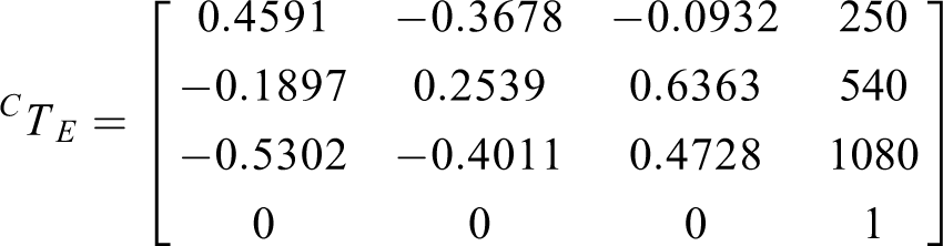
The 3-D coordinates of the end-effector and target object are obtained by the PCL acquisition, removing outliers, data compression, and so on. For the video (including 73 frames), the 3-D coordinates of the EECs are shown in Table 3. (x, y, z) denote space coordinates of EECs in the base coordinate frame. Before data compression, the TPC is shown in Figure 12(a). After data compression, the TPC is shown in Figure 12(b). The 3-D coordinates of the cylindrical TC are (214.2 mm, −3.9 mm, 825 mm).

Figure 12.

Fitting results. (a) TPC before data compression. (b) TPC after data compression. (c) Triangular facets and morphological processing.

Table 3.

3-D coordinates of EECs in base coordinate frame.

EEC (c) Frames (F)	x (mm)	y (mm)	z (mm)	Frames (F)	x (mm)	y (mm)	z (mm)	Frames (F)	x (mm)	y (mm)	z (mm)
1	0	0	0	26	211.5	−132.7	816.3	50	221.2	−62.7	816.6
2	211.3	−205.4	818.1	27	216.4	−130.9	815.2	51	221.7	−57.6	816.5
3	216.5	−201.4	818.1	28	214.9	−127.4	813.4	52	222.0	−54.0	815.3
4	215.5	−199.3	819.3	29	212.8	−124.9	809.7	53	217.9	−52.6	813.7
5	213.9	−196.0	821.5	30	217.8	−122.8	805.4	54	219.0	−50.5	813.8
6	215.3	−194.9	822.4	31	217.9	−116.7	805.3	55	214.4	−47.8	813.9
7	216.3	−188.6	823.0	32	210.8	−114.7	803.8	56	216.2	−44.7	813.6
8	215.5	−187.9	820.5	33	211.7	−111.9	803.4	57	217.3	−39.4	813.5
9	213.5	−185.1	820.2	34	223.3	−110.2	801.5	58	216.9	−38.4	813.7
10	221.3	−182.7	820.2	35	221.4	−107.7	801.6	59	215.9	−36.8	813.4
11	221.8	−177.0	819.0	36	222.0	−104.5	801.9	60	216.1	−34.4	813.3
12	222.8	−174.9	818.9	37	225.5	−99.5	801.2	61	215.4	−30.7	816.5
13	221.9	−173.1	816.0	38	221.6	−97.7	801.1	62	213.5	−27.8	816.6
14	221.3	−170.6	820.8	39	222.3	−94.8	801.5	63	217.2	−22.9	818.0
15	222.2	−167.0	818.9	40	219.6	−92.6	803.2	64	217.4	−19.7	820.1
16	219.0	−165.7	818.4	41	223.3	−89.0	803.4	65	211.0	−21.3	818.6
17	219.6	−159.4	820.4	42	221.2	−88.2	805.3	66	212.3	−18.0	818.5
18	214.8	−158.1	820.0	43	221.3	−84.7	805.1	67	214.7	−11.6	820.3
19	216.3	−157.1	818.0	44	222.9	−80.5	809.8	68	208.3	−8.8	818.3
20	210.8	−154.4	818.1	45	221.0	−78.1	813.9	69	209.3	−6.6	818.3
21	212.8	−151.3	820.6	46	220.8	−72.4	811.7	70	213.2	−3.2	820.2
22	214.3	−146.5	818.6	47	220.4	−71.1	811.9	71	211.4	−3.2	820.3
23	208.5	−143.9	820.3	48	220.1	−67.9	813.1	72	210.3	−3.4	823.3
24	209.2	−142.9	818.5	49	222.4	−65.6	815.3	73	212.6	−3.5	823.9
25	212.7	−139.9	816.3

From Table 3, the EEC gradually approaches the TC in the time domain. The absolute errors are 214.2 − 212.6=1.6 mm, −3.5−(−3.9) = 0.4 mm, and 825 − 823.9=1.1 mm along the x-, y-, and z-axes, respectively. The theoretical values are constant along the x-axis. But the experimental data fluctuate within a certain range. The maximum random fluctuation is 225.5 − 208.3 = 17.2 mm. The theoretical values decrease along the y-axis. The experimental data also decrease. The theoretical values increase along the z-axis. The trend of the experimental data is not increasing. The data are sometimes unchanged or fluctuant in some consecutive frames. The reason for the deviation is the low pixel accuracy of Kinect.

The deviation between the EEC and TC represents the positioning error. It provides reference data for the manipulator’s motion control. Under ideal conditions, the positioning is successful if the TC coordinates coincide with the EEC coordinates. But in the experiment, it is normal if there is a certain deviation. A known condition: The clamping mechanism has the maximum opening range 287 mm. According to the actual positioning requirement, the maximum permissible errors are 20 mm, 25 mm, and 20 mm along the x-, y-, and z-axes, respectively.

The surface fitting is implemented using triangular facets and morphological processing as shown in Figure 12(c). The article only shows the fitting results for the 5th, 25th_, 45th, 65th, and 73rd frames. This process verifies the correctness of the kinematic model and the effectiveness of the autonomous positioning algorithm. At the same time, it provides a convenient way for the visual monitoring of the positioning process.

Comparative analysis

In sections “Kinematics Analysis,” “End-effector State Estimation,” and “Target Recognition Experiment,” the active and passive objects are extracted from the scene based on the PF, BP recognition, and PCL technology. The position of the end-effector is adjusted using the error between the EECs and TC as a reference. Comparative experiments are carried out as shown in Table 4.

Table 4.

Algorithms comparison.

Parameters	Izadi et al.^1,7	Li et al.⁴	Lin et al.⁶	Hu and Li²⁸	Our method
Calculations	47,548	32,361	61,387	53,982	17,562
Time (s)	5.405	10.249	15.652	2.081	1.681
Subject to light source influence	Small	Larger	Larger	Small	Small
Reliance on mathematical modeling	Large	Larger	Larger	Large	Large
Reconstruction accuracy (mm)	0.15	0.40	0.19	0.15	0.15

The accumulated error cannot be corrected in the study by Izadi et al.¹ The 3-D reconstruction based on the monocular camera only relies on the mathematical model in the study by Li et al.⁴ The requirement for the light source is harsh. The 3-D reconstruction based on the binocular vision requires pattern matching and a lot of computations in the study by Lin et al.⁶ The effect of the reconstruction is significantly reduced in the case of a large baseline distance. The error of the position estimation is close to one reported in Carbone and Gomez-Bravo.⁹ The real time of the point cloud fitting is higher than that in the study by Kanatani et al.¹⁰ The recognition rate of 99% based on the BP neural network is higher than 90% based on the study by Gruen and Thomas.¹¹ The visual calibration is not required and calculations are clearly simplified in this article compared with that reported in Hu and Li.²⁸

The following conclusions are obtained from the comparative analysis.(I) Calculations are simplified using the PCL acquisition and data compression.(II) The hardware system has low light source demanding, mainly affected by direct sunlight. The reason is that Kinect uses near-infrared light. The solar spectrum interferes with Kinect.(III) The neural network recognition reduces the reliance on a mathematical model.(IV) The reconstruction accuracy is close to one reported in Izadi et al.¹ and Lin et al.⁶ The camera pixel accuracy, target recognition, and end-effector’s extraction all affect the accuracy of the surface fitting. In summary, the system efficiency improves significantly.

Conclusion

The article proposes a PF based on three-frame differencing to detect and track the end-effector’s motion in a static background. The target objects are identified based on the BP neural network classification idea. The coordinates of the TC are calculated. The positioning is successful when the positioning error is within an allowed range. Then, the TPC is collected based on the PCL technology. Outliers are removed, and data compression is carried out. The coordinate frame transforming model is established. TPCs are transformed into the base coordinate frame from the camera coordinate frame. Therefore, the coordinates are meaningful for the manipulator motion control. Finally, the surface fitting of the TPC is achieved.

Footnotes

Declaration of conflicting interests

The author(s) declared no potential conflicts of interest with respect to the research, authorship, and/or publication of this article.

Funding

The author(s) received no financial support for the research, authorship, and/or publication of this article.

References

Izadi

Newcombe

RA,

Kim

. Kinectfusion: real-time dynamic 3D surface reconstruction and interaction. Acm Siggraph 2011; 3(8): 23.

Xue

Yang

. Kinect-based real time 3D reconstruction of human and its application. J Comput Aided Des Comput Graph 2014; 26(10): 1720–1726.

Guo

Gao

. Batch reconstruction from UAV images with prior information. Acta Autom Sin 2013; 39(6): 834–845.

Yang

Qin

. Monocular camera three dimensional reconstruction based on optical flow feedback. Acta Opt Sin 2015; 35(5): 1–9.

Huang

Tao

. Dynamic Bayesian network model based golf swing 3D reconstruction using simple depth imaging device. J Electron Inf Technol 2015; 37(9): 2076–2081.

Lin

Lou

. Robot vision system for 3D reconstruction in low texture environment. Opt Precis Eng 2015; 23(2): 540–549.

Izadi

Kim

Hilliges

. Kinectfusion: real-time 3D reconstruction and interaction using a moving depth camera. ACM, Santa Barbara 2011: 559–568.

Kahl

Hartley

. Multiple-view geometry under the L_∞ norm. IEEE Trans Pattern Anal Mach Intell 2005; 30(9): 1603–1617.

Carbone

Gomez-Bravo

. Motion and operation planning of robotic systems. Mech Mach Sci 2015; 29(4): 15–26.

10.

Kanatani

Sugaya

Kanazawa

. Guide to 3D vision computation: geometric analysis and implementation. Advances in computer vision and pattern recognition. Springer International Publishing, 2016.

11.

Gruen

Thomas

. Calibration and orientation of cameras in computer vision. Springer series in information sciences. Springer Berlin Heidelberg, 2001; 34(3): 555–560.

12.

Martin

Robert

. Random sample consensus: a paradigm for model fitting with applications to image analysis and automated cartography. In: Graphics and Image Processing. Morgan Kaufmann Publishers, 1981, pp. 381–395.

13.

Andre

Christof

Robert

. 3D scene segmentation for autonomous robot grasping. In: 2012 IEEE/RSJ international conference on intelligent robots and systems, 2012, pp. 1734–1740. DOI: 10.1109/ IROS.2012.6385692.

14.

Suman

Mohammed

. A Gaussian process guided particle filter for tracking 3D human pose in video. IEEE Trans Image Process 2013; 22(11): 4286–4300.

15.

Refael

Richard

. Digital image processing, 2nd ed. University of Tennessee: Publishing House of Electronics Industry, 2002.

16.

Chang

Hsiao

JY,

Hsieh

. An adaptive median filter for image denoising. Elsevier B.V. 2008; 39(11): 346–350.

17.

Liu

Lin

, Image edge detection algorithm based on mathematical morphology. J South China Univ Technol (National Science Edition) 2008; 36(9): 113–116.

18.

Shi

Cai

XJ,

Zhu

. Ship target identification based on the wavelet transform and neural network. Syst Eng Electron 2004; 26(7): 893–895.

19.

Liu

You

. A neural network for image object recognition and its application to car type recognition. Comput Eng 2003; 29(3): 30–32.

20.

Hao

Jiang

. Training sample selection method for neural networks based on nearest neighbor rule. Acta Autom Sin 2007; 33(12): 1247–1251.

21.

Richard

Shahram

Otmar

. KinectFusion: real-time dense surface mapping and tracking. In: IEEE international symposium on mixed and augmented reality 2011 science and technology proceedings, 2011, pp. 127–136. DOI:10.1109/ISMAR.2011.6092378.

22.

Zhu

Cao

Yang

. An improved Kinectfusion 3D reconstruction algorithm. Robot 2016; 36(2): 129–136.

23.

Shao

Wang

. Denoising method of 3D point cloud data of plants obtained by Kinect. Trans Chin Soc Agric Mach 2016; 47(1): 331–335.

24.

Merry

Marais

Gain

. Compression of dense and regular point clouds. Comput Graph Forum 2006; 25(4): 709–716.

25.

Ivan

Marten

Petter

. Intrinsic camera and hand-eye calibration for a robot vision system using a point marker. In: 14th IEEE-RAS international conference on humanoid robots, 18–20 November 2014, pp. 59–66. DOI: 10.1109/HUMANOIDS.2014.7041338.

26.

. Series actuator end integrated positioning analysis based on multilayer perception neural network. Trans Chin Soc Agric Eng Academic Press Professional,Inc.: San Diego, CA, USA, 2016; 1(32): 22–27.

27.

Bloomenthal

. An implicit surface polygonizer. In: Graphics Gems IV. San Diego, CA: Academic Press Professional Inc., 1994, pp. 324–349.

28.

. 3D reconstruction of end-effector in autonomous positioning process using depth imaging device. Math Probl Eng 2016; 2016(10): 1–16.

Autonomous positioning control of manipulator and fast surface fitting based on particle filter and point cloud library technology

Abstract

Keywords

Introduction

End-effector motion estimation

Object recognition

Image preprocessing

Neural network recognition

Autonomous positioning

Point cloud acquisition

Point cloud processing

TPC data compression

Coordinate frames transforming

Experiment and analysis

Kinematics analysis

End-effector state estimation

Target recognition experiment

Positioning experiment

Comparative analysis

Conclusion

Footnotes

Declaration of conflicting interests

Funding

References