Design of a cable-driven hyper-redundant robot with experimental validation

Abstract

This article presents a test bed for comprehensive study of a cable-driven hyper-redundant robot in terms of mechanical design, kinematics analysis, and experimental verification. To design the hyper-redundant robot, the multiple section structure is used. Each section consists of two rotational joints, a link mechanism, and three cables. In this sense, two degrees of freedom are achieved. For kinematics analysis between the actuator space and joint space, each section of the development is treated as three spherical–prismatic–spherical chains and a universal joint chain (3-SPS-U), which results in a four-chain parallel mechanism model. In order to obtain the forward kinematics from the joint space to task space directly and easily, the coordinate frames are established by the geometrical rules rather than the traditional Denavit–Hartenburg (D-H) rules. To solve the problem of inverse kinematics analysis, we utilize the product of exponentials approach. Finally, a prototype of 24-degrees of freedom hyper-redundant robot with 12 sections and 36 cables is fabricated and an experiment platform is built for real-time control of the robot. Different experiments in terms of trajectories tracking test, positioning accuracy test, and payload test are conducted for the validation of both mechanical design and model development. Experiment results demonstrate that the presented hyper-redundant robot has fine position accuracy, flexibility with mean position error less than 2%, and good load capacity.

Introduction

Traditional industrial robots generally consist of several serially connected links and joints, which are usually actuated by motors mounted on joints. They have been proved to be efficient in many application scenarios but also reveal some intrinsic limitations, for instance, lack of flexibility and degrees of freedom (DOF). ¹ Alternatively, hyper-redundant robots show a wide range of flexibility. In comparison with traditional robots, they have a larger number of DOFs which make them very suitable for applications in unconstructed and clamped environments. ² Thus, they may play a critical role in inspection and maintenance of complex industrial devices such as aircraft wings, ³ engines, nuclear reactors, and pipelines ^4,5 ; search and rescue operations in disaster situation; ⁶ and minimally invasive surgery (MIS) instruments. ^{7 –9}

Many hyper-redundant robot mechanisms have been designed, which can be roughly classified into two categories: rigid-backbone robots and continuum-backbone robots. ^10,11 The flexibility of rigid-backbone robots is determined by the number of joints and the length of links of the robots. For example, the active chord mechanism developed by Shigeo et al. ¹² which was composed of a large number of segments and joints was the pioneer work of rigid-backbone hyper-redundant robots. Recently, OC robotics, ³ a company in United Kingdom, developed several commercial this kind of robots, which were successfully applied to the inspection of nuclear reactor. Yang et al. ¹³ designed an anthropomimetic 7-DOFs cable-driven robotic arm which had the similar workspace of human arm. Li et al. ^14,15 developed a constrained wire-driven flexible robot consisting of many under-actuated joints and nodes. The other kind of hyper-redundant robots is the continuum-backbone robot which was coined by Robinson and Davies ¹⁶ first. The flexible materials the robots occupy such as spring, elastic rod, and so on make them flexible. For instance, the OctArm designed by McMahan et al. ¹⁷ was actuated by pneumatic muscle. It was dexterous and could manipulate objects. Dong et al. ¹¹ developed a slender continuum-backbone robot composed of twin-pivot compliant joints, in which the whole section served as a universal joint. Xu and Simaan ⁹ developed a throat surgery system driven by Ni–Ti alloy tendons, which could conduct some dexterous operations such as suture. Webster and Dupont ^7,8 developed the concentric tube continuum robots which were driven by pre-curved concentric tube. The small size and flexibility of the concentric tubes made them proper for MIS. While many hyper-redundant robots are used in the application of MIS, ¹⁸ there are also some successful application cases in industry. For example, the snake-arm systems developed by OC robotics ¹⁹ have been utilized for inspection and maintenance in nuclear plants (Ringhals BWR, Sweden, 2004 and CANDU reactors, Canada, 2010). A concept of snake-like robot has been implemented by Tesla ²⁰ to automatically charge for electric cars. The slender continuum robotic system developed by Dong and Axinte ²¹ has been used for on-wing inspection of gas turbine engines.

It is of crucial importance to develop an accurate mathematical model for the hyper-redundant robot since it is the basis for predicting the robot’s motion, responses, and designing model-based controllers. Due to the complicated parallel–serial hybrid structures, there are large numbers of DOFs in the hyper-redundant robot, which makes the commonly used modeling methods of traditional industrial robot not applicable. To tackle this problem, three kinds of methods have been proposed in recent years. Walker et al., ¹⁰ Chirikjian and Burdick, ²² Hirose and Yamada, ² and Choset et al. ¹⁸ adopted the parameterized backbone curves to describe the shape of hyper-redundant robots. Hannan and Walker ¹ and Webster and Jones ²³ presented the constant curvature model for continuum robots. Recently, Yang et al. ¹³ and Li et al. ²⁴ employed the screw theory and product of exponential (POE) formula to model the hyper-redundant continuum robots.

However, robots in some industrial applications under confined environment should take flexibility, accuracy, and payload capability as paramount. There is little literature comprehensively including the design, analysis, and experimental validation of such robots. Therefore, this article conducts the following research to reach the above goals. To this end, a cable-driven hyper-redundant robot is designed in this work. As discussed in Dong et al., ¹¹ the twist problem should be carefully taken into consideration in the design of the hyper-redundant robot in order to keep its load/force capability. We utilize a kind of structure with two rotational joints in each section. With this concept, a hyper-redundant robot prototype which owns 12 sections and 24 joints is developed with a diameter/length ratio of 0.036. To drive the robotic manipulator effectively, a novel compact and efficient transmission mechanism is built. The kinematics coordinate frames are set based on the geometrical rules rather than the commonly used Denavit–Hartenburg (D-H) rules to simplify its kinematics analysis. To establish the mapping from the actuator space to the joint space, a spherical–prismatic–spherical (SPS) chains and a universal joint chain (3-SPS-U) parallel mechanism model is proposed. It is well-known that traditional differential and inverse kinematics are challenging for this kind of hyper-redundant robots because of massive DOFs. To address this challenge, the POE approach is employed for the differential and inverse kinematics analysis of hyper-redundant robots. Finally, sufficient experiments are conducted to verify the designed mechanism and kinematic models. Experiment results indicate that the robot possesses advantages in terms of good flexibility and fine accuracy.

The rest of this article is organized as follows: “Design of the robot” section describes the design of the hyper-redundant manipulator and transmission mechanism. The kinematics mappings among the actuator space, joint space, and task space of the robot are derived in “Kinematics of the hyper-redundant robot” section. “Jacobian and differential inverse kinematics using POE formula” section notifies the Jacobian and differential inverse kinematics of the robot using POE formula. The developed prototype and validation experiments are presented in “Experimental validation” section. The sixth section concludes this article.

Design of the robot

The 3-D model of the developed hyper-redundant robot which consists of a cable-driven robotic manipulator and an actuation system is shown in Figure 1. The cable-driven robotic manipulator owes 12 sections with 24 DOFs. The actuation system is comprised of a transmission mechanism, motors, and electronic boards. In the following, detailed descriptions of the development will be presented.

Figure 1.

Schematic of the whole system of the robot.

Robotic manipulator design

The cable-driven manipulator is composed of 12 2-DOF sections, where each section consists of a link, two disks, and two rotational joints as shown in Figure 2. There are central holes in all the components, forming a central large lumen to go through electrical wires as seen in the local enlarged image in Figure 2. To illustrate the development clearly, Figure 3 denotes the detailed structure of each section. It can be seen that two disks are connected to the two ends of the link, respectively. One rotational joint is attached to the distal disk, and another rotational joint is connected with the former one with their origins coincided, making their rotational axes intersect perpendicularly. In order to achieve the 2-DOFs motion, cables are used to drive the two rotational joints. Adjacent sections are connected by the second joint in the previous section and the proximal disk in the next section. Finally, the multi-section manipulator can be fabricated by stacking many sections together.

Figure 2.

Developed cable-driven robotic manipulator.

Figure 3.

Illustration of a section of the cable-driven manipulator.

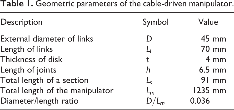
The cables not only transmit mechanical power to the manipulator of the robot but also connect sections. As shown in Figure 3, they are fixed to the end of a proximal disk in a section. The intrinsic compliance of cables makes the robot compliant. To control the rotation of the two joints in each section, three or four cables can be adopted. ¹³ However, four cables will make the transmission mechanism bulky. In this work, three evenly distributed cables are used. The stress in the cables will increase rapidly with the increase of the rotation angles. To protect the joint mechanism and avoid huge stress of the cable, mechanical limitations are set above and under the joints. Under the constraints of mechanical limitations, the maximal rotation angles about axes are 54°. Geometric parameters of the designed robot are summarized in Table 1.

Table 1.

Geometric parameters of the cable-driven manipulator.

Description	Symbol	Value
External diameter of links	D	45 mm
Length of links	Ll	70 mm
Thickness of disk	t	4 mm
Length of joints	h	6.5 mm
Total length of a section	Ls	91 mm
Total length of the manipulator	Lm	1235 mm
Diameter/length ratio	D/Lm	0.036

Actuation system design

The designed manipulator is driven by the actuation system. As shown in Figure 1, the actuation system composed of transmission mechanism, motors, and electronic boards is placed external to keep the robot compact and efficient. In addition, it is versatile and can be used to drive different types of cable-driven manipulators of various sizes. The motors are connected to the transmission mechanism, and the steel cables with a diameter of 1 mm are also attached to it.

To transmit power from massive motors to cables, a novel compact and versatile transmission mechanism is developed, which consists of 36 transmission modular units. As shown in Figure 4, each unit consists of a coupling, a bearing seat, a ball screw, a linear slide, a fixture of cables, a connection nut, and a supporting board. The bearing seat and linear slide are mounted on the supporting board, and the ball screw is set on the bearing seat with the couplings attached to it. The connection nut connects the ball screw, linear slide, and the fixture of cables together. At last, the end of a cable is fixed in the fixture of cables. As shown in Figure 1, all the transmission units are assembled on the pedestal and evenly distributed along the circumference. When the actuation system works, the cables should keep stretched and tight, for they can only transmit tension instead of contraction. As a result, the motors’ movements change the lengths of the cables, causing the manipulator to move.

Figure 4.

Rendering diagram of transmission unit.

Kinematics of the hyper-redundant robot

Based on the designed structure, the kinematics analysis of the hyper-redundant robot can be achieved by considering each section of the manipulator individually. The position and orientation of each section are determined by the rotation of the joints, and the rotation angles are controlled by cables. Hence, the kinematics can be divided into two mappings among three spaces, which is shown in Figure 5. The lengths of cables are defined as the actuator space. The rotation angles of each section are notified as the joint space, and the position and orientation of the tip of the robot are described as the task space. g ₁ and $g_1^{-1}$ are forward and inverse kinematics between actuator space and joint space, respectively. Similarly g ₂ and $g_2^{-1}$ are forward and inverse kinematics between joint space and task space, respectively.

Figure 5.

Kinematics mapping between three spaces.

Mapping from the actuator space to the joint space

The cable lengths change only between the distal disk in the previous section and the proximal disk in the next section, while cable lengths in links remain the same. As a result, mapping from the actuator space to the joint space mainly concerns the region between distal disk in previous section and proximal disk in next section. Figure 6 shows the geometric illustration of the area between two sections. Regular triangle ABC coincides with the surface of the distal disk in previous section. The cables pass the distal disk through A, B, and C. Point O is the center of the distal disk. H is the origin of the two rotational joints. The first joint connected with the distal disk by OH, and the second joint connected with the proximal disk by HO ₁. The cables pass through the proximal disk and fastened at A ₁, B ₁, and C ₁, respectively.

Figure 6.

Geometric illustration of the area between two sections.

The whole section can be seen as a parallel mechanism with the lower platform ABC; upper platform A ₁ B ₁ C ₁; and four chains AA ₁, BB ₁, CC ₁, and OO ₁. The disks have no orientation constrains at the connected points with the cables, which means the cables can rotate about any direction at the connected point with disks. Hence, the connection between cable and disk can be viewed as a spherical joint. Moreover, the cable can elongate along its direction, which can be treated as a prismatic joint. Therefore, chains AA ₁, BB ₁, and CC ₁ can be seen as SPS chains. Chain OO ₁ is comprised of a universal joint and moves passively along with three other chains. Thus, a single section can be regarded as a 3-SPS-U parallel mechanism, in which three SPS are active chains and U is the passive chain. As a result, g ₁ and $g_1^{-1}$ are the forward and inverse kinematics of a parallel mechanism. To simplify the kinematics analysis, the coordinate frames are established according to the geometric rules. ^25,26 As shown in Figure 6, the coordinate frames are set as follows:

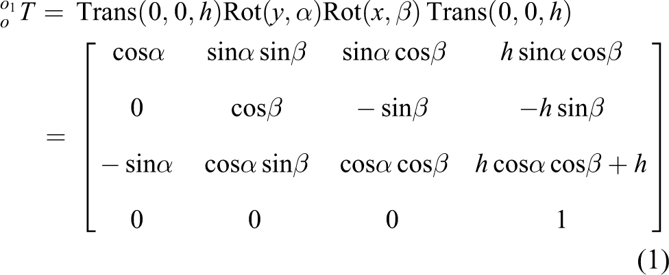
Joint coordinate systems are defined as Φ ₁ ={X ₁ , Y ₁ , Z ₁} and Φ ₂ ={X ₂ , Y ₂ , Z ₂}. Φ ₁ and Φ ₂ are attached to the first and second joints, respectively, with their origins set at point H. Axes Y ₁ and X ₂ coincide with the rotational axes of the first and second joints, respectively. Axes Z ₁ and Z ₂ are parallel to the central axis of the link in the next section. The axes X ₁ and Y ₂ are determined according to the right-hand rule.

Lower platform coordinate system is designated as Φ_l = {X_l, Y_l, Z_l }. It is attached to distal disk in previous section with its origin set at point O, and the XY plane coincides with surface ABC. X_l is aligned with OA, and Z_l is aligned with OH.

Upper platform coordinate system is defined as Φ_u = {X_u, Y_u, Z_u }. It is attached to proximal disk in next section with its origin set at point O ₁, and the XY plane coincides with surface A ₁ B ₁ C ₁. X_u is aligned with O ₁ A ₁, and Z_u is aligned with HO ₁.

Parameters of the mechanism are described as follows: l_a , l_b , and l_c are the lengths of the three driving cables, and r is the radius of the circumcircle of triangles ABC and A ₁ B ₁ C ₁. The distance between the joints and the disks is equal, satisfying |OH| = |OH₁| = h. Under such coordinate frames, the homogenous coordinates of the points on disks are as follows: O = (0, 0, 0, 1)^T, H = (0, 0, h, 1)^T, A = (r, 0, 0, 1)^T, B = (−r/2, − $\sqrt{3}/2$ r, 0, 1)^T, and C = (−r/2, $\sqrt{3}/2$ r, 0, 1)^T. Euler angles of the two joints are defined as (α, β), in which α and β are the rotation angles about Y ₁ and X ₂ axes, respectively. According to the above coordinate frames and parameters, the transformation matrix between lower and upper platforms can be expressed as

$\begin{array}{l}{}_o{}^{o_1}T=\text{Trans}(0,0,h)Rot(y,\alpha )Rot(x,\beta )\text{Trans}(0,0,h)\\ =\left[\begin{array}{cccc}\cos \alpha & \sin \alpha \sin \beta & \sin \alpha \cos \beta & h\sin \alpha \cos \beta \\ 0& \cos \beta & -\sin \beta & -h\sin \beta \\ -\sin \alpha & \cos \alpha \sin \beta & \cos \alpha \cos \beta & h\cos \alpha \cos \beta +h\\ 0& 0& 0& 1\end{array}\right]\end{array}$

1

Transformation relationships between points on adjacent disks are as follows: $O_1={}_o{}^{o_1}\mathit{T}\mathit{O}_{ }^{ },{\mathit{A}}_1={}_o{}^{o_1}\mathit{T}\mathit{A}_{ }^{ },{\mathit{B}}_1={}_o{}^{o_1}\mathit{T}\mathit{B}_{\hspace{0.17em}}^{\hspace{0.17em}},\hspace{0.17em}\text{and}\hspace{0.17em}{C}_1={}_o{}^{o_1}\mathit{T}\mathit{C}_{ }^{ }$ . Hence, the lengths of cables can be obtained through geometrical relationship between vectors in Figure 6, which are as follows

$l_a^2={\overrightarrow{A{A}_1}}^2={(\overrightarrow{AO}+\overrightarrow{OH}+\overrightarrow{H{O}_1}+\overrightarrow{O_1{A}_1})}^2=2r^2+2h^2+\overrightarrow{AO}\cdot \overrightarrow{H{A}_1}+\overrightarrow{OH}\cdot \overrightarrow{H{A}_1}$

2

$l_b^2={\overrightarrow{B{B}_1}}^2={(\overrightarrow{BO}+\overrightarrow{OH}+\overrightarrow{H{O}_1}+\overrightarrow{O_1{B}_1})}^2=2r^2+2h^2+\overrightarrow{BO}\cdot \overrightarrow{H{B}_1}+\overrightarrow{OH}\cdot \overrightarrow{H{B}_1}$

3

$l_c^2={\overrightarrow{C{C}_1}}^2={(\overrightarrow{CO}+\overrightarrow{OH}+\overrightarrow{H{O}_1}+\overrightarrow{O_1{C}_1})}^2=2r^2+2h^2+\overrightarrow{CO}\cdot \overrightarrow{H{C}_1}+\overrightarrow{OH}\cdot \overrightarrow{H{C}_1}$

4

Lengths of the cables can be determined by substituting coordinate of the above points into equations (2) to (4). As a result, the inverse kinematics mapping from the actuator space to the joint space $g_1^{-1}$ is defined by equations (1) to (4). The relationships among cable lengths can be obtained as follows

$l_a^2+l_b^2+l_c^2=6r^2+6h^2+3\overrightarrow{OH}\cdot \overrightarrow{H{O}_1}+\overrightarrow{AO}\cdot \overrightarrow{O_1{A}_1}+\overrightarrow{BO}\cdot \overrightarrow{O_1{B}_1}+\overrightarrow{CO}\cdot \overrightarrow{O_1{C}_1}$

5

$l_c^2-l_b^2=\overrightarrow{OH}\cdot \overrightarrow{B_1{C}_1}+\overrightarrow{BC}\cdot \overrightarrow{H{O}_1}+\overrightarrow{CO}\cdot \overrightarrow{O_1{C}_1}-\overrightarrow{BO}\cdot \overrightarrow{O_1{B}_1}$

6

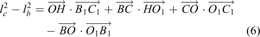
Notice that to obtain equations (5) and (6), the relationships $\overrightarrow{H{A}_1}+\overrightarrow{H{B}_1}+\overrightarrow{H{C}_1}=3\overrightarrow{H{O}_1}\hspace{0.17em}\text{and}\hspace{0.17em}\overrightarrow{AO}+\overrightarrow{BO}+\overrightarrow{CO}=0$ are used.

By substituting coordinates of related points to equations (5) and (6), one can obtain

$l_a^2+l_b^2+l_c^2=6r^2+6h^2+3h^2\text{cos}\alpha \text{cos}\beta -1.5r^2\text{cos}\alpha -1.5r^2\text{cos}\beta$

7

$l_c^2-l_b^2=\sqrt{3}hr\text{cos}\alpha \text{sin}\beta +\sqrt{3}hr\text{sin}\beta +\sqrt{3}/2(r^2\text{sin}\alpha \text{sin}\beta )$

8

To acquire α and β, equations (7) and (8) can be rearranged by

$\text{cos}\beta =\frac{l_a^2+l_b^2+l_c^2-6r^2-6h^2+1.5r^2\text{cos}\alpha }{3h^2\text{cos}\alpha -1.5r^2}$

9

$\text{sin}\beta =\frac{l_c^2-l_b^2}{\sqrt{3}/2(r^2\text{sin}\alpha )+\sqrt{3}hr(\text{cos}\alpha +1)}$

10

According to ${\text{sin}}^2\beta +{\text{cos}}^2\beta =1$ , $\text{sin}\alpha =\frac{2u}{1+u^2}$ , and $\text{cos}\alpha =\frac{1-u^2}{1+u^2}$ , equations (9) to (10) can be rewritten as the equation in terms of u. First, some coefficients of u are denoted by parameters of l_a , l_b , l_c , h, and r as follows

$\begin{array}{l}{b}_1=(l_c^2-l_b^2)(3h^2+1.5r^2)\\ b_2=(l_c^2-l_b^2)(3h^2-1.5r^2)\\ b_3=l_a^2+l_b^2+l_c^2-9h^2-9r^2\\ b_4=l_a^2+l_b^2+l_c^2-3h^2-6r^2\\ b_5=l_a^2+l_b^2+l_c^2-9h^2-3r^2\end{array}$

11

$\begin{array}{l}{a}_8=b_1^2\\ a_7=0\\ a_6=2b_1^2-2b_1{b}_2+3r^4{b}_3{b}_4\\ a_5=12h{r}^3{b}_3{b}_4\\ a_4=b_1^2+4b_1{b}_2+b_2^2+12h^2{r}^2{b}_3{b}_4+3r^4(b_4^2+b_3{b}_5)\\ a_3=12h{r}^3(b_4^2+b_3{b}_5)\\ a_2=2b_2^2-2b_1{b}_2+12h^2{r}^2(b_4^2+b_3{b}_5)+3r^4{b}_4{b}_5\\ a_1=12h{r}^3{b}_4{b}_5\\ a_0=b_2^2+12h^2{r}^2{b}_4{b}_5\end{array}$

12

Hence, the equation about u can be denoted as follows

$a_8{u}^8+a_7{u}^7+a_6{u}^6+a_5{u}^5+a_4{u}^4+a_3{u}^3+a_2{u}^2+a_{1}u+a_0=0$

13

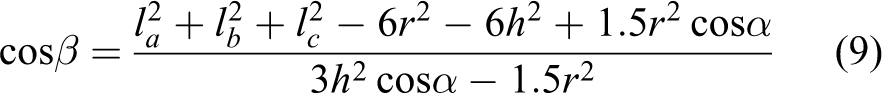
The solution of equation (13) is u, and α can be denoted as

$\alpha =2{\text{tan}}^{-1}u$

14

Substituting equation (14) into equations (9) and (10), rotational angle β can be expressed as

$\beta =A\text{tan}2(\text{sin}\beta ,\text{cos}\beta )$

15

Hence, the forward kinematics mapping from the actuator space to the joint space g ₁ is defined by equations (14) and (15).

Mapping from the joint space to the task space

The mapping from joint space to task space is related to rotation angles of the joints and position and orientation of the end effector of the robot. Thus, coordinate frames are attached to each joint.

As shown in Figure 7, coordinate frames are set by geometrical rules as the same way in mapping from the actuator space to the joint space. Φ_i = {X_i , Y_i , Z_i } is the coordinate frame of a section which coincides with the coordinate frame of the second joint of the section. ¹ Φ_{i −1} = {¹ X_{i −1}, ¹ Y_{i −1}, ¹ Z_{i −1}} and ² Φ _i−1 = {² X_{i −1}, ² Y_{i −1}, ² Z_{i −1}} are the transition coordinate frames between Φ_{i −1} and Φ_i . ¹ Φ_{i −1} is gotten by translating Φ_{i −1} along Z _{i −1} by 2h + L, where h is the length of the joint and L represents the total length of a link and two disks. ² Φ_{i −1} is obtained by rotating ¹ Φ_{i −1} about ¹ Y _{i −1} by α_i , and Φ_i is gotten by rotating ² Φ_{i −1} about ¹ X _{i −1} by β_i . Thus, the transformation matrix between Φ_{i −1} and Φ_i is

$\begin{array}{l}{{}_{i-1}{}^{i}T}_1=\text{Trans}(0,0,2h+L)Rot(y,{\alpha }_i)Rot(x,{\beta }_i)\\ =\left[\begin{array}{cccc}\cos {\alpha }_i& \sin {\alpha }_i\sin {\beta }_i& \sin {\alpha }_i\cos {\beta }_i& 0\\ 0& \cos {\beta }_i& -\sin {\beta }_i& 0\\ -\sin {\alpha }_i& \cos {\alpha }_i\sin {\beta }_i& \cos {\alpha }_i\cos {\beta }_i& 2h+L\\ 0& 0& 0& 1\end{array}\right]\end{array}$

16

Figure 7.

Coordinate frames by geometrical rules.

To verify the effectiveness and validity of the geometrical model, the mechanism is modeled by commonly used D-H rules. Coordinate frames are established according to D-H rules shown in Figure 8. The beginning and end frames in Figure 8 are the same as those in Figure 7. D-H parameters in each section are in Table 2. Transformation matrix between adjacent sections derived by D-H rules is equation (17)

$\begin{array}{c}{}_{i-1}{}^{ i}T_2^{ }=\text{Trans}(0,0,2\mathit{h}+\mathit{L})\text{Rot}(\mathit{x},-{90}^{\circ })\text{Rot}(\mathit{z},{90}^{\circ }+{\alpha }_i)\text{Rot}(\mathit{x},{90}^{\circ })\\ \text{Rot}(z,{180}^{\circ }+{\beta }_i)\text{Rot}(x,{90}^{\circ })\text{Rot}(z,{90}^{\circ })\text{Rot}(x,{90}^{\circ })\end{array}$

17

Figure 8.

Coordinate frames by D-H rules. D-H: Denavit–Hartenburg.

Table 2.

D-H parameters of a section.

	a	α	d	θ
1	0	−90°	2h + L	0
2	0	90°	0	90° + αi
3	0	90°	0	180° + βi
4	0	90°	0	90°

D-H: Denavit–Hartenburg.

It can be proved that the geometric rules and D-H rules get the same result. However, geometric rules are more easy and straightforward to derive the transformation matrix. The coordinate frames established by geometric rules are quite helpful for the kinematics using POE formula which will be illustrated in “Jacobian and differential inverse kinematics using POE formula” section. As a result, the forward kinematics from the joint space to task space g ₂ can be described as

${}_w{}^{n}T_1^{ }={}_w{}^1\mathit{T}_1^{ }{}_1{}^2\mathit{T}_1^{ }\cdot \cdot \cdot {}_{i-1}{}^{ i}T_1^{ }\cdot \cdot \cdot {}_{\mathit{n}-1}{}^{ n}\mathit{T}_1^{ }$

18

where ${}_w{}^{1}T$ is the transformation matrix of the first link frame related to the world frame. The inverse kinematics is challenging because of hyper-redundancy of the mechanism. On the other hand, inverse kinematics of single section is easy and will be analyzed. The inverse kinematics of whole manipulator will be tackled by differential inverse kinematics and Jacobian matrix using POE formula in the rest of this article.

If the positions of all the joints are known, the rotational angles of each section can be derived. $\overrightarrow{z_i}$ and $\overrightarrow{z_{i-1}}$ are defined as the Z axis of section i and i−1, respectively. With angles ${\alpha }_1,\mathrm{...},{\alpha }_{i-1}\hspace{0.17em}\text{and}\hspace{0.17em}{\beta }_1,\mathrm{...},{\beta }_{i-1}$ are known, $\overrightarrow{z_i}$ and $\overrightarrow{z_{i-1}}$ can be transformed to the position where $\overrightarrow{z_{i-1}}$ equals to ${(0,0,1)}^{\text{T}}$ . The relationship between them is

$\overrightarrow{z_i}=\left[\begin{array}{c}{x}_i\\ y_i\\ z_i\end{array}\right]=\left[\begin{array}{ccc}\text{cos}{\alpha }_i& \text{sin}{\alpha }_i\text{sin}{\beta }_i& \text{sin}{\alpha }_i\text{cos}{\beta }_i\\ 0& \text{cos}{\beta }_i& -\text{sin}{\beta }_i\\ -\text{sin}{\alpha }_i& \text{cos}{\alpha }_i\text{sin}{\beta }_i& \text{cos}{\alpha }_i\text{cos}{\beta }_i\end{array}\right]\overrightarrow{z_{i-1}}$

19

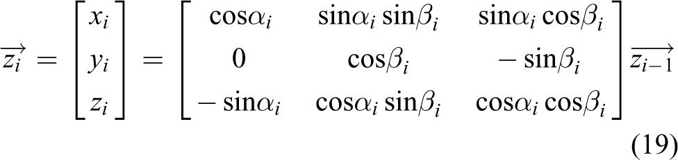
The range α_i and β_i is −27° to +27°, and hence, they can be determined uniquely according to equation (19)

$\begin{array}{c}{\alpha }_i=\text{arcsin}(x_i/\text{cos}({\beta }_i))\\ {\beta }_i=\text{arcsin}(-y_i)\end{array}$

20

The inverse kinematics of single section is described by equation (20), which is helpful for developing motion planning methods for the hyper-redundant robots. As discussed in Andersson, ²⁷ with all the position of the joints are determined, the angles of the joints can be calculated according to equation (20) in a recursive way.

Jacobian and differential inverse kinematics using POE formula

Kinematics denoted by equations (16) and (18) are useful for forward kinematics and single section inverse kinematics, but there is no analytic solution for the inverse kinematics of the whole manipulator. Meanwhile, Jacobian and differential inverse kinematics by partial differentiation of equations (16) and (18) are generally difficult because of massive DOFs. However, the geometrical coordinate is intuitive for the POE formula to derive Jacobian and differential inverse kinematics of hyper-redundant robot. In addition, POE approach has the advantages of compact form, geometric significance of the twist, and ease of implementation, ^28,29 which are suitable for Jacobian and differential inverse kinematics of our hyper-redundant robot.

Introduction of POE formula

The position and orientation of link i−1 frame X_{i −1} Y_{i −1} Z_{i −1} relative to link i frame X_iY_iZ_i are described by ${\Psi }_{i,i\text{-1}}\text{=}{M}_i{e}^{P_i{\mathit{\theta }}_i}$ , in which $M_i\in SE(3)$ is the initial position and orientation of frame X_{i −1} Y_{i −1} Z_{i −1} relative to frame X_iY_iZ_i , and ${\mathit{\theta }}_i\in R$ is the joint variable. $\mathit{\omega },v\in R^3$ , $\xi ={\left[\begin{array}{cc}{\mathit{\omega }}^{\text{T}}& v^{\text{T}}\end{array}\right]}^{\text{T}}$ is the vector representation of lie algebra and is also the twist described in the screw motion of matrix $e^{P_i{\mathit{\theta }}_i}$ , where

$\widehat{\mathit{\omega }}={\left[\begin{array}{c}{\mathit{\omega }}_1\\ {\mathit{\omega }}_2\\ {\mathit{\omega }}_3\end{array}\right]}^{^}=\left[\begin{array}{ccc}0& -{\mathit{\omega }}_3& {\mathit{\omega }}_2\\ {\mathit{\omega }}_3& 0& -{\mathit{\omega }}_1\\ -{\mathit{\omega }}_2& {\mathit{\omega }}_1& 0\end{array}\right]\in so(3),\hspace{0.17em}{P}_i=\left[\begin{array}{cc}\widehat{\mathit{\omega }}& v\\ 0& 0\end{array}\right]=\widehat{\xi }\in se(3)$

where ∧ is the hat operator mapping a vector to a skew symmetric matrix. The matrix representation of lie algebra of SE(3) is P_i . The exponential mapping transforming $P\in se(3),\mathit{\theta }\in R$ to $e^{P\mathit{\theta }}\in SE(3)$ is an operator that maps twist to screw motion in local coordinate frames. The mapping formulas are as follows

$e^{P\mathit{\theta }}\text{=}{e}^{\left[\begin{array}{cc}\widehat{\mathit{\omega }}\mathit{\theta }& v\mathit{\theta }\\ 0^T& 0\end{array}\right]}=\left[\begin{array}{cc}{e}^{\widehat{\mathit{\omega }}\mathit{\theta }}& Vv\\ 0^T& 1\end{array}\right]$

21

$e^{\widehat{\mathit{\omega }}\mathit{\theta }}=I+\text{sin}\mathit{\theta }\widehat{\mathit{\omega }}+(1-cos\mathit{\theta }){\widehat{\mathit{\omega }}}^2$

22

$V=\mathit{\theta }I+(1-\text{cos}\mathit{\theta })\widehat{\mathit{\omega }}+(\mathit{\theta }-\text{sin}\mathit{\theta }){\widehat{\mathit{\omega }}}^2$

23

Then, the forward kinematics between joints space to task space of the manipulator using POE formula can be denoted as

$\Psi ({\mathit{\theta }}_1,\cdot \cdot \cdot ,{\mathit{\theta }}_i,\cdot \cdot \cdot ,{\mathit{\theta }}_n)=e^{N_1{\mathit{\theta }}_1}{e}^{N_2{\mathit{\theta }}_2}\cdot \cdot \cdot e^{N_i{\mathit{\theta }}_i}\cdot \cdot \cdot e^{N_n{\mathit{\theta }}_n}N$

24

To present the twist of the joints in different coordinate frames clearly, ${\xi }_i={P_i}^{\vee }$ and ${\xi }_i^{\prime }={N_i}^{\vee }$ are employed to denote the twists in local and world frame, respectively. The relationship between twists in local and world frames P_i and N_i can be denoted as $N_i=A{d}_{M_1\cdot \cdot \cdot M_i}{P}_i=\widehat{{\xi }_i^{\prime }}$ . A more easy and straightforward way to obtain the twist in the world frame ${\xi }_i^{\prime }$ is to adjoint transformation of the vector representation of lie algebra ${\xi }_i$ . ³⁰ R and p are defined as

$M_1\cdot \cdot \cdot M_i=\left[\begin{array}{cc}R& p\\ 0& 1\end{array}\right],R\in SO(3),p\in R^3$

then

${\xi }_i^{\prime }=\left[\begin{array}{cc}R& 0\\ \widehat{p}R& R\end{array}\right]{\xi }_i$

25

where, $\widehat{p}$ is the result of hat operator of p.

Kinematics using POE formula

Based on the coordinate frames established by the geometrical rules as in “Kinematics of the hyper-redundant robot” section, the POE formula is adopted to obtain the Jacobian and differential inverse kinematics of the robot. With different world frames, the POE formulas can be divided to local POE and global POE. ³¹

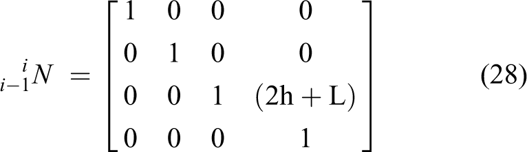
Firstly, the kinematics transformation matrix between adjacent sections ${}_{i-1}{}^{i}T$ is derived by local POE formula, in which the world frame is coincided with frame X_i− ₁ Y_i− ₁ Z_i− ₁. The twist in the local coordinate frames in each section can be denoted as ${\xi }_{yi}^i={(0,1,0,0,0,0)}^{\text{T}},{\xi }_{xi}^i={(1,0,0,0,0,0)}^{\text{T}}$ , when the initial joint angles are 0. Initial conditions between the ith frame and the world frame are M_i = (R, p), R = I, and p = (0, 0, h)^T. According to equation (25), the twists of two rotation axes of ith frame in the world coordinate frames in section i are ${\xi }_{yi}^{i-1}={(0,1,0,-(2h+L),0,0)}^{\text{T}}\hspace{0.17em}\text{and}\hspace{0.17em}{\xi }_{xi}^{i-1}={(1,0,0,0,2h+L,0)}^{\text{T}}$ . Screw motions matrices of the two joints in section i related to frame X_{i −1} Y_{i −1} Z_{i −1} are equations (26) and (27), according to equations (21) to (23). The result of equation (29) describes the kinematics of a single section

$e^{\widehat{{\xi }_{yi}^{i-1}}{\alpha }_i}=\left[\begin{array}{cccc}\text{cos}{\alpha }_i& 0& \text{sin}{\alpha }_i& -(2h+L)\text{sin}{\alpha }_i\\ 0& 1& 0& 0\\ -\text{sin}{\alpha }_i& 0& \text{cos}{\alpha }_i& (2h+L)(1-\text{cos}{\alpha }_i)\\ 0& 0& 0& 1\end{array}\right]$

26

$e^{\widehat{{\xi }_{xi}^{i-1}}{\beta }_i}=\left[\begin{array}{cccc}1& 0& 0& 0\\ 0& \text{cos}{\beta }_i& -\text{sin}{\beta }_i& (2h+L)\text{sin}{\beta }_i\\ 0& \text{sin}{\beta }_i& \text{cos}{\beta }_i& (2h+L)(1-\text{cos}{\beta }_i)\\ 0& 0& 0& 1\end{array}\right]$

27

${}_{i-1}{}^{ i}N_{ }^{ }=\left[\begin{array}{cccc}1& 0& 0& 0\\ 0& 1& 0& 0\\ 0& 0& 1& (2h+L)\\ 0& 0& 0& 1\end{array}\right]$

28

${{}_{i-1}{}^{i}T}_3=e^{\stackrel{\wedge }{{\xi }_{yi}^{i-1}}{\alpha }_i}{e}^{\stackrel{\wedge }{{\xi }_{xi}^{i-1}}{\beta }_i}{}_{i-1}{}^{i}N$

29

Secondly, the first link coordinate X ₁ Y ₁ Z ₁ is taken as the world frame, which is called the global POE. The initial conditions between the ith frame and the world frame are ${}_1{}^{i}M=(R,{}_1^{i}p),R=I$ , and ${}_1{}^{n}p={(0,0(i-1)(2h+L))}^{\text{T}}$ when the initial joint angles are 0. According to equation (25), twists of two rotation axes of ith frame in world coordinate frames in section i are ${\xi }_{yi}^1={(0,1,0,-(i-1)(2h+L),0,0)}^{\text{T}}$ and ${\xi }_{xi}^1={(1,0,0,0,(i-1)(2h+L),0)}^{\text{T}}$ . Screw motions matrices of the two joints in section i related to frame X ₁ Y ₁ Z ₁ are equations (30) and (31).

$e^{\widehat{{\xi }_{yi}^1}{\alpha }_i}=\left[\begin{array}{cccc}\text{cos}{\alpha }_i& 0& \text{sin}{\alpha }_i& -(i-1)(2h+L)\text{sin}{\alpha }_i\\ 0& 1& 0& 0\\ -\text{sin}{\alpha }_i& 0& \text{cos}{\alpha }_i& (i-1)(2h+L)(1-\text{cos}{\alpha }_i)\\ 0& 0& 0& 1\end{array}\right]$

30

$e^{\widehat{{\xi }_{xi}^1}{\beta }_i}=\left[\begin{array}{cccc}1& 0& 0& 0\\ 0& \text{cos}{\beta }_i& -\text{sin}{\beta }_i& (i-1)(2h+L)\text{sin}{\beta }_i\\ 0& \text{sin}{\beta }_i& \text{cos}{\beta }_i& (i-1)(2h+L)(1-\text{cos}{\beta }_i)\\ 0& 0& 0& 1\end{array}\right]$

31

${}_1{}^{n}N_{ }^{ }=\left[\begin{array}{cccc}1& 0& 0& 0\\ 0& 1& 0& 0\\ 0& 0& 1& (\mathit{n}-1)(2\mathit{h}+\mathit{L})\\ 0& 0& 0& 1\end{array}\right]$

32

${{}_w{}^{n}T}_2=e^{\stackrel{\wedge }{{\xi }_{y1}^1}{\alpha }_1}{e}^{\stackrel{\wedge }{{\xi }_{x1}^1}{\beta }_1}\cdot \cdot \cdot e^{\stackrel{\wedge }{{\xi }_{yi}^1}{\alpha }_i}{e}^{\stackrel{\wedge }{{\xi }_{xi}^1}{\beta }_i}\cdot \cdot \cdot e^{\stackrel{\wedge }{{\xi }_{yn}^1}{\alpha }_n}{e}^{\stackrel{\wedge }{{\xi }_{xn}^1}{\beta }_n}{}_1{}^{n}N$

33

As a result, equation (33) is the forward kinematics of the robot derived by POE formula, which has advantages of compact, Lie theoretic foundations, and so on. In addition, computation of the forward kinematics and Jacobian is much more efficient than other methods, which has been proved by Park. ²⁸ Hence, it is very promising to use the POE formula for Jacobian and differential inverse kinematics of the hyper-redundant robot.

Jacobian analysis and resolution of redundant inverse kinematics of the robot

Once the forward kinematics has been established by POE formula, Jacobian and differential inverse kinematics can be derived as follows. The spatial velocity of the tip of the manipulator is

$\widehat{V_s}=\stackrel{•}{{{}_w{}^{n}T}_2}{}_w{}^{n}T_2^{-1}={\displaystyle \sum _{i=1}^n(\frac{\partial {{}_w{}^{n}T}_2}{\partial {\alpha }_i}}{}_w{}^{n}T_2^{-1}\stackrel{•}{{\alpha }_i}+\frac{\partial {{}_w{}^{n}T}_2}{\partial {\beta }_i}{}_w{}^{n}T_2^{-1}\stackrel{•}{{\beta }_i})$

34

By partial differentiating the transformation matrices in terms of each joint angle, factors in equation (34) can be denoted as

$\begin{array}{l}\frac{\partial {{}_w{}^{n}T}_2}{\partial {\alpha }_i}{}_w{}^{n}T_2^{-1}=e^{\stackrel{\wedge }{{\xi }_{y1}^1}{\alpha }_1}{e}^{\stackrel{\wedge }{{\xi }_{x1}^1}{\beta }_1}\cdot \cdot \cdot e^{\stackrel{\wedge }{{\xi }_{yi-1}^1}{\alpha }_{i-1}}{e}^{\stackrel{\wedge }{{\xi }_{xi-1}^1}{\beta }_{i-1}}(\stackrel{\wedge }{{\xi }_{yi}^1})e^{-\stackrel{\wedge }{{\xi }_{xi-1}^1}{\beta }_{i-1}}{e}^{-\stackrel{\wedge }{{\xi }_{yi-1}^1}{\alpha }_{i-1}}\cdot \cdot \cdot e^{-\stackrel{\wedge }{{\xi }_{x1}^1}{\beta }_1}{e}^{-\stackrel{\wedge }{{\xi }_{y1}^1}{\alpha }_1}\\ \frac{\partial {{}_w{}^{n}T}_2}{\partial {\beta }_i}{}_w{}^{n}T_2^{-1}=e^{\stackrel{\wedge }{{\xi }_{y1}^1}{\alpha }_1}{e}^{\stackrel{\wedge }{{\xi }_{x1}^1}{\beta }_1}\cdot \cdot \cdot e^{\stackrel{\wedge }{{\xi }_{yi-1}^1}{\alpha }_{i-1}}{e}^{\stackrel{\wedge }{{\xi }_{xi-1}^1}{\beta }_{i-1}}{e}^{\stackrel{\wedge }{{\xi }_{yi}^1}{\alpha }_i}(\stackrel{\wedge }{{\xi }_{xi}^1})e^{-\stackrel{\wedge }{{\xi }_{yi}^1}{\alpha }_i}{e}^{-\stackrel{\wedge }{{\xi }_{xi-1}^1}{\beta }_{i-1}}{e}^{-\stackrel{\wedge }{{\xi }_{yi-1}^1}{\alpha }_{i-1}}\cdot \cdot \cdot e^{-\stackrel{\wedge }{{\xi }_{x1}^1}{\beta }_1}{e}^{-\stackrel{\wedge }{{\xi }_{y1}^1}{\alpha }_1}\end{array}$

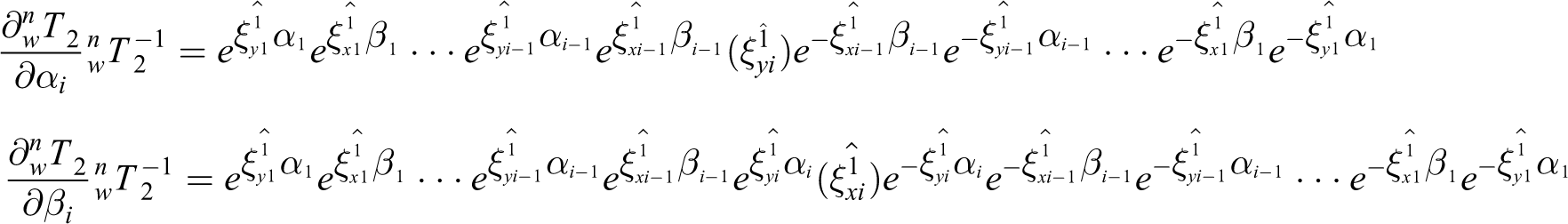
Hence, the twists of Y and X axis of section i undergone rigid motion are equations (35) and (36), respectively.

${\xi }_{yi}^{1\prime }={\left(\frac{\mathit{\partial }{}_w{}^{n}T_2^{ }}{\mathit{\partial }{\alpha }_i}{}_w{}^{n}T_2^{-1}\right)}^{\vee }=A{d}_{(e^{\widehat{{\xi }_{y1}^1}{\alpha }_1}{e}^{\widehat{{\xi }_{x1}^1}{\beta }_1}\cdot \cdot \cdot e^{\widehat{{\xi }_{yi-1}^1}{\alpha }_{i-1}}{e}^{\widehat{{\xi }_{xi-1}^1}{\beta }_{i-1}})}{\xi }_{yi}^1$

35

${\xi }_{xi}^{1\prime }={\left(\frac{\mathit{\partial }{}_w{}^{n}T_2^{ }}{\mathit{\partial }{\beta }_i}{}_w{}^{n}T_2^{-1}\right)}^{\vee }=A{d}_{(e^{\widehat{{\xi }_{y1}^1}{\alpha }_1}{e}^{\widehat{{\xi }_{x1}^1}{\beta }_1}\cdot \cdot \cdot e^{\widehat{{\xi }_{yi-1}^1}{\alpha }_{i-1}}{e}^{\widehat{{\xi }_{xi-1}^1}{\beta }_{i-1}}{e}^{\widehat{{\xi }_{yi}^1}{\alpha }_i})}{\xi }_{xi}^1$

36

Twists of joints undergone rigid motion are ${\xi }_{yi}^{1\prime }$ and ${\xi }_{xi}^{1\prime }$ which are expressed in equations (35) and (36), respectively. They are adjoint transformation of twists ${\xi }_{yi}^1$ and ${\xi }_{xi}^1$ . Therefore, the vector representation of spatial velocity of the end effector is

$V_s={(\stackrel{•}{{{}_w{}^{n}T}_2}{}_w{}^{n}T_2^{-1})}^{\vee }={\displaystyle \sum _{i=1}^n((\frac{\partial {{}_w{}^{n}T}_2}{\partial {\alpha }_i}}{}_w{}^{n}T_2^{-1}{)}^{\vee }\stackrel{•}{{\alpha }_i}+{(\frac{\partial {{}_w{}^{n}T}_2}{\partial {\beta }_i}{}_w{}^{n}T_2^{-1})}^{\vee }\stackrel{•}{{\beta }_i})=J_s(\theta )\stackrel{•}{\theta }$

37

The spatial Jacobian of the robot is

$J_s(\mathit{\theta })=\left[\begin{array}{cccccccc}{\xi }_{y1}^{1\prime }& {\xi }_{x1}^{1\prime }& \cdot \cdot \cdot & {\xi }_{yi}^{1\prime }& {\xi }_{xi}^{1\prime }& \cdot \cdot \cdot & {\xi }_{yn}^{1\prime }& {\xi }_{xn}^{1\prime }\end{array}\right]$

38

$\mathit{\theta }={\left[\begin{array}{cccccccc}{\alpha }_1& {\beta }_1& \cdot \cdot \cdot & {\alpha }_i& {\beta }_i& \cdot \cdot \cdot & {\alpha }_n& {\beta }_n\end{array}\right]}^{\text{T}}$

39

We can see that each column of the spatial Jacobian matrix is the expression in the world frame of the twist undergone rigid motion from equation (38). Thus, the calculation of the spatial Jacobian becomes straightforward.

The Jacobian is not square and has no inverse because of the redundancy. However, the generalized Moore–Penrose pseudo inverse $J_s^{+}={J_s}^{\text{T}}{\left(J_s{J_s}^{\text{T}}\right)}^{-1}$ can be used to the inverse kinematics of the robot. ¹⁰ As a result, the inverse kinematics can be denoted as

$\stackrel{•}{\mathit{\theta }}={J_s}^{+}\stackrel{•}{x}$

40

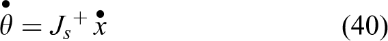
where $\dot{x}$ is the velocity of the end effector.

The redundancy makes it difficult to get the inverse of the Jacobian. However, the null space of J_s can be utilized to optimize the joint angles without changing the positon and orientation of the end effector. The orthogonal projection matrix in the null space of J_s is I − J_s ⁺ J_s , thus the inverse kinematics equation (40) can be rewritten as

$\stackrel{•}{\mathit{\theta }}={J_s}^{+}\stackrel{•}{x}\text{+(}{I}_{24}-{J_s}^{+}{J}_s\text{)}\nabla Q(\mathit{\theta })$

41

As a result, the inverse kinematics between joint space and task space $g_2^{-1}$ of the robot is denoted by equation (41), where ∇Q(θ) can be any arbitrary velocity of joint space. In this case, Q(θ) is the criterion function of all joint angles needing to be optimized. Besides∇Q(θ) is the gradient of function Q(θ), which can be set as follows

$Q(\mathit{\theta })={\displaystyle \sum _{i=1}^n(({\mathit{\theta }}_i}-{\mathit{\theta }}_{ai})/{\mathit{\theta }}_{mi}{)}^2$

42

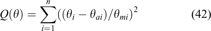
where θ_i is the value of ith joint angle, θ_ai is the average value of the maximal and minimal value of ith joint angle, and θ_mi is equal to θ_ai subtract the maximal value of joint angle.

Experimental validation

In this section, a prototype of the proposed cable-driven hyper-redundant robot is fabricated and experiments are conducted for the verification of the designs and kinematics analysis.

Experiment setup

The experiment platform is shown in Figure 9. The manipulator is controlled by the motors (Maxon EC-MAX30 with rated power of 60W and rated speed of 6590 rpm) with EPOS2 boards. The kinematics model of the hyper-redundant robot is simulated on the MATLAB (R2015a) developed by MathWorks, and the path-planning is performed based on the developed kinematics models. Figure 10 shows the prototype of the robot with 12 sections. Each section of the manipulator is made of aluminum alloy. The maximal rotation angle of each section of the prototype is ±27°, and the maximal gross rotation angle of manipulator is about 320°.

Figure 9.

Block diagram of the experiment platform.

Figure 10.

Prototype of the developed hyper-redundant robot.

Trajectories tracking

The developed hyper-redundant robot is adopted to keep track of various trajectories such as circles and five-pointed stars. In order to visualize the path that the end effector of the robot has passed, a pencil is attached to the tip of the robot. Figure 11 shows the results of drawing a circle with a diameter of 72 mm by taking 15 s. In this sense, the speed of the end effector is of 15.07 mm/s. As an illustration, the configurations of the robot at 3 s, 6 s, 9 s, and 12 s are depicted in Figure 11 respectively.

Figure 11.

Hyper-redundant robot keep track of a circle.

In another test, a trajectory of five-point star with a side length of 60 mm is tracked with the developed hyper-redundant robot. The experiment results are shown in Figure 12, where the configurations of the robot at 30 s, 50 s, 70 s, and 90 s are presented, respectively. In this test, the robot takes 100 s to finish the task, and the speed of the end effector is of 3 mm/s.

Figure 12.

Hyper-redundant robot keep track of a five-point star.

Positioning accuracy test

In order to evaluate the position accuracy of the developed models, the robot is controlled to follow different desired trajectories. For example, the circle drawn by the robot in “Trajectories tracking” section is used to analyze the positioning accuracy.

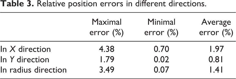
For a quantitative comparison, Figure 13(b) shows both the recorded and desired trajectories. It should be mentioned that the recorded data are scanned into images as shown in Figure 13(a), which are dealt with MATLAB. Figure 14 shows the tracking errors between the desired and recorded data. It can be seen that the average position errors of X, Y, and radius direction are less than 2%, which clearly verifies the accuracy of the development. In summary, Table 3 lists the maximal, minimal, and average relative position errors of X, Y, and radius directions.

Figure 13.

Circle drawn by the robot: (a) scanned image of the drawn circle and (b) recorded and desired MATLAB data.

Figure 14.

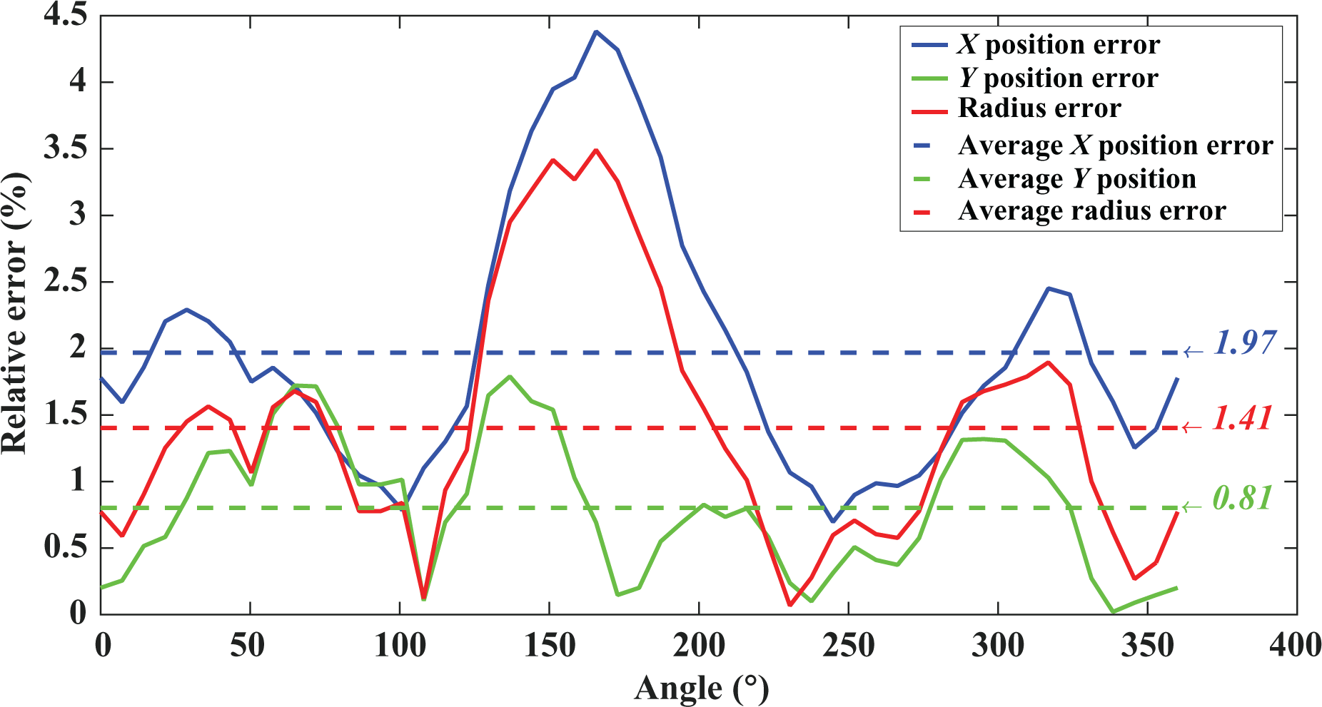
Relative positioning errors of distal positions.

Table 3.

Relative position errors in different directions.

	Maximal error (%)	Minimal error (%)	Average error (%)
In X direction	4.38	0.70	1.97
In Y direction	1.79	0.02	0.81
In radius direction	3.49	0.07	1.41

Payload test

In order to preliminarily test the payload capability of the development, the robot draws some lines without and with external exerted payloads. Figure 15(a) shows the results of payload tests, when the robot is planned to draw a line with 500 g weight exerted on the tip of the manipulator. Figure 15(b) is the enlarged view of Figure 15(a). The above line in Figure 15(b) is the line the manipulator draw without payload, and the below line is drawn by the manipulator with 500 g payload.

Figure 15.

Payload tests: (a) lines drawn by the robot. The upper line is drawn without payload, and the lower line is drawn under 500 g payload; (b) the enlarged view of the drawn lines.

It can be seen the two lines are almost parallel, and the line drawn by the robot with payload is some centimeters offset below the above one. Major reason for the offset may lies in the fact that the manipulator possesses a length as long as 1235 mm and the pre-stretch force is not enough. The long length will enlarge the moment exerted on the other end of the manipulator when the payload exerted on the tip of it. The manipulator will deviate downward because of the inadequate pre-stretch force. The experiment result shows that the payload has little influence on the shape of the trajectories of the tip of the manipulator, with some offset between them.

It should be noted that in this work, the maximal velocity of the end effector of the robot is kept to be less than 16 mm/s. In this sense, the dynamics of the robot may be ignored in the performance analysis. Therefore, all the performance analysis is based on the kinematic model of the robot. Of course, with the increase of the velocity, the dynamics of the robot should be taken into consideration, which will be our future work. Another assumption for the performance analysis is that the steel cables have no elastic deformation, and they keep straight and tight all the time.

Conclusion and discussion

This article presents a kind of slender cable-driven hyper-redundant robot which is composed of a slim manipulator and a compact actuation system. The developed 24-DOFs manipulator can move dexterously with maximal bending angle of 320° and diameter/length ratio as small as 45mm/1235 mm. To control the robot effectively, the kinematics model of the robot is established. First, the kinematics coordinate frames of the robot are established by geometric rules. Second, kinematics mappings among actuator space, joint space, and task space are derived by transformation matrix and POE formula. A 3-SPS-U parallel mechanism model is proposed to establish the mapping from the actuator space to the joint space. At last, to verify the designs and kinematics analysis, a prototype is developed. Experiments such as keeping track of trajectories, positioning accuracy, and payload test are carried out. The experiment results show that fine position accuracy is achieved by the developed robot with average tracking error less than 2% when it draws a circle with a radius of 72 mm.

In the future, the positioning accuracy can be further improved by parameters calibration and feedback control of the robot by adopting sensors in the manipulator. Motion planning of the robot will be conducted for the inspection of confined environment. To compensate for the effects caused by the exerted payload, statics and dynamics models based on feedforward and feedback control approaches should be taken.