
Abstract
Physical human–robot interaction may present an obstacle to transparency and operations’ intuitiveness. This barrier could occur due to the vibrations caused by a stiff environment interacting with the robotic mechanisms. In this regard, this article aims to deal with the aforementioned issues while using an observer and an adaptive gain controller. The adaptation of the gain loop should be performed in all circumstances in order to maintain operators’ safety and operations’ intuitiveness. Hence, two approaches for detecting and then reducing vibrations will be introduced in this study as follows: (1) a statistical analysis of a sensor signal (force and velocity) and (2) a multilayer perceptron artificial neural network capable of compensating the first approach for ensuring vibrations identification in real time. Simulations and experimental results are then conducted and compared in order to evaluate the validity of the suggested approaches in minimizing vibrations.
Keywords
Introduction
Physical human–robot interaction (pHRI) has become an interesting option in the industry for handling and assembling. 1 In fact, it has a potential to produce a positive impact in assisting and sharing tasks in scheduling production and manufacturing activities while ensuring greater reliability, flexibility and precision. 2 –4 However, robot’s stability and dynamic transparency may present a safety risk. 5,6 Indeed, physical contact with a force sensing handle could generate vibrations coming from an increase of the loop gain (i.e. vibrations generated by the approach of the poles towards the imaginary axis) which reduce performance, transparency and operations’ intuitiveness. 7 Thus, to remedy problems related to the application of this concept, several control models have been developed for reducing mechanical vibrations and then ensuring safe and intuitive pHRIs. 8,9
Following a review of the art in technologies used for reducing vibrations and analysing mechanisms’ stabilities, we will describe the primary contribution of this study; a design of an intelligent observer based on an artificial neural network (ANN) approach for minimizing mechanical vibrations in pHRIs in real time. For that, we will begin by representing a model of a pHRI and its analysis based on an adaptive closed-loop control system. Moreover, two observers based on a statistical analysis and an ANN will be elaborated for detecting and minimizing vibrations. These observers are evaluated and compared for different human arm stiffness. This evaluation provides a choice of an appropriate strategy for minimizing mechanical vibrations in pHRIs.
Related work
This section is an introduction to the most used control and observers models, in the context of pHRIs, aimed at satisfying mechanisms’ intuitiveness, performance and stability in all circumstances. First, we begin by presenting two types of control loops used in pHRIs and then, we will finish with the neural network observers.
Impedance and admittance controls
Admittance and impedance controls are the most known control techniques in pHRIs. 9 These techniques are applied in two different mechanisms. Impedance control is a force control model that takes a measurement of displacement as an input and reacts with a force as an output. 10 In contrast, admittance control takes a force as an input and reacts with a displacement as an output. 11,12 Furthermore, unlike admittance control, impedance control is the most common force control model used in the literature for mechanisms characterized by a low inertia and limited friction. 13 This last point makes the impedance control improper for collaborating with the intelligent assist device (IAD) used in this work, since it is characterized by a high level of inertia and friction. These later make it too difficult for an operator to confer a movement to the IAD shown in both Figures 1 and 2. An admittance controller with positional feedback is therefore preferred in this study.

Control scheme.

Intelligent assistive device.
To remedy issues of robotic mechanisms’ instabilities related to the human arm stiffness which is varying depending on the difficulty of the hand task, 9 some precursors, such as Tsumugiwa et al., 14 explored an impedance control technique to vary the damping coefficient. This addition of damping is based on the estimated value of the human arm stiffness. In the same context, Ikeura and Inooka 15 used a variable impedance control method depending on the threshold of the mechanisms’ velocity. In addition, Lecours et al. 13 used a variable admittance control method based on human intentions inference while using the desired speed and acceleration. Furthermore, Corteville et al. 16 detailed a technique using the admittance control based on an estimation of operators’ planned movements. Finally, Duchaine and Gosselin 9 detailed a new approach of a robust controller aiming at ensuring a greater stability of interactive robotic mechanisms and intuitive interactions. Such improvement was done thanks to a combination of observer stability and a variable admittance control depending on human intentions.
Adaptive controller using an observer
Regarding the challenge of ensuring safe and intuitive pHRIs, one popular stability controller has been developed using the passivity approach. Such a solution has been used, principally, in haptics 17 and, more recently, in the context of pHRIs. 9,18 The main idea is to ensure an efficient measurement of the device’s energy flow. This measure provides an index to which we refer for accurate and efficient information on the system’s state. 19 Thus, if mechanism’s instability occurs, we can use a passive controller absorbing exactly the energy measured by an observer through a dissipative element (i.e. damping coefficient).
This tool has been used by several researchers in different applications. In fact, some studies used the concept of the passivity to guarantee the stability control of a teleoperation with force feedback. 20,21 Colgate and Schenkel 22 were interested in processing a virtual wall characterized by virtual settings such as stiffness and damping. Moreover, Hannaford and Ryu 19 tested the passivity concept while doing a simulation and an implementation on a haptic device. Ryu et al. 23 have used the same principle introduced in the study by Hannaford and Ryu 19 but took into account the variation of the speed during a sample period. Similarly, Ryu et al. 24 called into question the principle of the passivity to ensure the stability of a commercial haptic device, labelled ‘PHANToM’, while varying the desired energy threshold in the time. Furthermore, Ryu et al. 25 proposed a new approach consisting in realizing a stability observer able to detect haptic system instabilities through an analysis of its movements in the frequency domain. This observer may also quantify the instabilities’ degree used thereafter by a stability controller to adapt a damping coefficient included in a dissipative element. However, these observers are not working with an admittance controller to move large payloads as demonstrated in our previous study. 26 Indeed, this previous study has shown that the energy computation does not measure the increase of vibrations as a function of the human arm stiffness for the IAD. Therefore, we suggest an algorithm able to measure the quantity of vibrations in order to adapt the control parameters such as the virtual mass and the gain loop. Routh–Hurwitz stability criterion was analysed on the minimal virtual mass rendered at the end effector. 27
ANN observer
Another solution for reducing mechanical vibrations is the so-called neural network vibration observer. This concept has been mainly used in detecting and minimizing vibrations affecting the normal lifetime of industrial equipment and causing the industry very high tooling costs. In this context, Rao et al. 28 studied the tool wear, surface roughness and vibrations of work pieces in boring of AISI 316 steel with cemented carbide tool inserts. For that, an experimental data acquisition of work pieces vibrations was conducted to a feedforward four-layered backpropagation neural network. Thus, it was concluded that the proposed network model was a smart instrument for predicting the tool wear, surface roughness and amplitude of vibrations. Consequently, it will be possible to change tools at the correct time in order to get good quality of products and to minimize tooling costs.
Moreover, Barszcz et al. 29 were interested in developing a new approach for decreasing the cost of wind turbine maintenance. To do so, they tested an adaptive resonance theory neural network as a tool for classifying vibration signals of bearing in gears in wind turbines. Furthermore, Kawabe et al. 30 proposed an active vibrations damping technique using a three-layered neural network controller, a strain gauge sensor and an actuator in a longitudinal type cantilever beam. In this study, it was found that the neural network control system was robust against weight parameter variations. Afterwards, Ali et al. 31 explained a new approach for monitoring and diagnosing rolling element bearings to ensure the steadiness of industrial and domestic machineries. Therefore, a four-layered neural network was constructed and trained with the recorded and the adjusted vibration signals. Based on these results, this article suggests using the neural network as a stability observer in order to design an adaptive gain controller.
Contribution
This article presents simulations and experimental results on the stability of an IAD through an ANN, labelled in the following active vibration observer (AVO). This AVO is designed for measuring and then reducing mechanical vibrations, generated in pHRIs, below the threshold of the human perception. Such process could increase operator safety, transparency and operations’ intuitiveness. The aforementioned observer will generate an index from a given signal with robustness to noise and human arm stiffness. This index will be used as a skillful means for performing an automatic adjustment of the control loop gain as a function of the detected mechanical vibrations in order to achieve our objectives in reducing such vibrations and in avoiding performance’s reductions in normal operations.
Modelling human–robot interaction
The mathematical models used to represent the pHRI are presented below. First, the admittance transfer function is presented, then the IAD model is detailed and finally the closed-loop control strategy is developed.
Admittance model
For ensuring greater transparency of the IAD which is coupled to a load, admittance model will be used. This model allows a force display (i.e. using a virtual mass and damping) that we want to be felt by the operators interacting with the robot instead of the real mass and damping. The one-dimensional second-order differential equation, used in this study, is written as follows 13,27 (the IAD is supposed to be isotropic 32 )

where fH is the interaction force felt by the hand, mv is the virtual mass, cv is the virtual damping, x0 is the equilibrium point and
To simulate free motions, it is assumed that stiffness kv, equilibrium position x0, equilibrium velocity

The desired velocity (set-point) can be written in the Laplace domain as follows 27,33
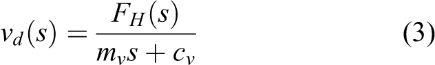
where s is the Laplace variable and vd(s) and FH(s) are the Laplace transforms of
The control scheme used in this work is presented in Figure 1
27,33
and the IAD is presented in Figure 2. The operator, wishing to make a displacement via the robot model, generates a force measured by means of a force/torque sensor located in the handle, labelled sensing handle in Figure 1. This measure, as well as the constrained velocity
Robot model
The robot model used for the experiments reported in this article is the four-degree-of-freedom (4-DOF) IAD prototype allowing translation in all directions (X, Y and Z, which are isotropic) and rotation about the vertical axis as seen in Figure 2. The moving mass, approximately 500 kg, is in the direction of the X-axis. Gravity is compensated using a balancing system with passive external mass (without control). The transmission between the actuators and the end effector consists in a transmission belt as illustrated schematically in Figures 2 and 3, where mR is the motor–belt translation inertia and x1 is its position; CB is the mechanical transmission damping; KB is the stiffness (i.e. CB and KB represent the transmission belt); CR is the viscous friction generated when moving the load MR, with the sensing handle; and x2 is its position, v2 is the measured velocity of the IAD in the feedback loop as shown in Figure 4, FH and F are the interaction force (i.e. the force applied by the operator) and the actuation force sent to the IAD actuators, respectively, and X0 is the visual target desired by the operator.

Intelligent assist device model.

Suggested control loop model without observers.
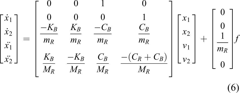
From Lecours and Gosselin, 8 the mechanical equations of this model are written as follows


Since the operator should not fell the load, equation (5) is equal to zero, otherwise it is equal to fH(t). Thus, equations (4) and (5) lead to the following state space representation
Suggested control loop model
The suggested control loop model is represented in Figure 4. 13 This model assumes that the operator acts as a spring damping system where KH is the operator stiffness and CH is the operator damping coefficient. 34 This operator generates a force FH as a function of the visual target. After that, FH will be transferred to a desired velocity vd by means of an admittance model, explained in equation (3). Moreover, a transfer function called Imperfections is also added where T represents a phase. This transfer function represents the effect of signal filtering, the errors of robot dynamics modelling and small delays. 13 The result of the Imperfections will be then sent to a velocity controller Kp (i.e. the control loop gain) which will be adjusted by our suggested algorithm. Finally, the resulting command F will be sent to the IAD actuators with a possible perturbation P (e.g. when a moving part of the IAD touches an object not related to the load). Classical PID is not used here since stability analysis is only performed on the loop gain.
The transfer function of the closed-loop model shown in Figure 4 can be written as follows
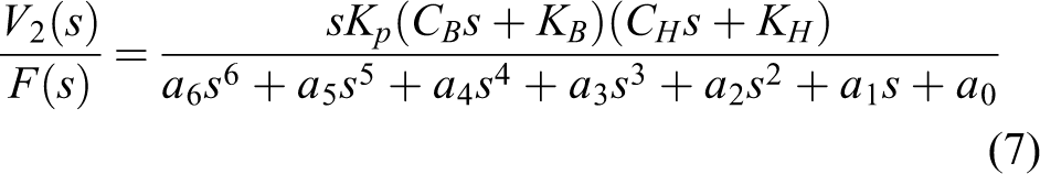
where

In the following, we will analyse the stability of the closed-loop transfer function, equation (7), using the position of its poles in the complex s-plane (i.e. complex plane on which Laplace transforms are graphed) along with the root locus stability criterion (i.e. graphical method for examining how the roots of a system change with variations of a certain system parameter which is in our case the operator stiffness KH and the loop gain Kp). This latter is represented in Figure 5, where the pole starting points are represented by a circle and the parameter variation is represented by a square.

Poles of the closed-loop model from equation (7) for an operator stiffness KH, varying from 50 N/m (circle) to 850 N/m (square), c = 20 Ns/m, T = 0.1 s, Kp = 10000, MR = 500 kg, CR = 100 Ns/m, mR = 50 kg, KB = 40000 N/m, CB = 40 Ns/m and CH = 23.45 Ns/m. These values are taken from Alexandre et al. 27
Based on the result, shown in Figure 5, we learn that greater operator stiffness leads to a more underdamped system. Accordingly, greater operator stiffness can lead to an unstable system; however, in the most common situation, it leads to a vibratory system (i.e. poles become near to the imaginary axis). The system stability, here, is justified by the fact that the poles are located on the left-hand side (i.e. negative part) of the Laplace plane. It should be pointed out that some of the poles shown in Figure 5 correspond to high frequencies (30 rad/s) and are very underdamped.
Thus, the operator will perceive the vibrations and then the interaction will be counterintuitive and uncomfortable. In fact, an increase of the loop gain (i.e. coming from an increase of the arm stiffness KH) could move the poles to an unstable position.
Stability observers
This section discusses how to detect and reduce mechanical vibrations by observing the velocity signal (v2) of a 1-DOF reduced-scale robot captured by means of a velocity sensor shown in Figure 6. Hence, two approaches, namely a statistical analysis, using both the time and the frequency domains, and an ANN are presented below.

1-DOF device used to evaluated the signal analysis prior to the IAD implementation. DOF: degree of freedom; IAD: intelligent assistive device.
It should be pointed out that the velocity signal used to analyse the pHRI (i.e. vibrations and instability as described in the preceding sections) is captured from a 1-DOF robot prototype (Figure 6) allowing the translation only in the X-direction, and the moving mass is much more lower than the 4-DOF IAD prototype shown in Figure 2, which allows much more higher vibrations frequencies. This analysis was first made to help us verify the validity of our algorithm. The stability analysis of this minimum phase system was previously presented in the study by Alexandre et al. 27
Statistical analysis
This analysis consists in assessing the electric signal representing the velocity of the movement of the mass in both the time and the frequency domains through a statistical analysis. For the frequency representation, the discrete Fourier transform could be applied using the fast Fourier transform algorithm (FFT) which is known for its limited computation operations 25 and its inability to deal with the problems that pose non-stationary and non-periodic signals. 35 A short-time FFT (ST-FFT) is therefore preferred to analyse a short period of the signal through a Hamming sliding window.
The velocity signal and its transformation after filtering, used in this study, are shown in Figure 7, where zones 1 and 3 correspond to a normal situation (i.e. without vibrations) and zone 2 corresponds to an abnormal situation (i.e. with vibrations). In zone 3, the handle is not held by the operator.
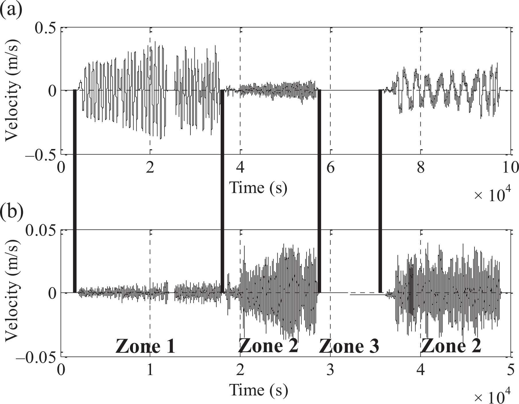
Signal measured from 1-DOF device: (a) the captured velocity signal and (b) its transformation after filtering (removing the arm movement) where zones 1 and 3 correspond to a vibrations-free situation and zone 2 corresponds to a vibratory situation. DOF: degree of freedom.
To analyse the dynamics and the frequency behaviours of the IAD with equations (6) and (7), we used the bode plot. This plot, represented in Figure 8, shows the dynamics of the following four parts:
the open-loop transfer function (Figure 8(a)),
the closed-loop transfer function (Figure 8(b)),
the human model transfer function (Figure 8(c)) and
the IAD transfer function (Figure 8(d)).

Bode plots representing the dynamics of (a) the closed-loop control, (b) the open-loop control, (c) the human and (d) the IAD (without control). As described here, vibrations then should occur at 0.15 and 30 rad/s. IAD: intelligent assistive device.
It is found that a resonance peak is present on the gains’ curves of the closed loop, the open loop and the IAD which reflects the vibratory behaviour created by the robot. Such behaviour is driven by the presence of the human arm stiffness in the control loop. In fact, the operator, wishing to control the manipulator of the robot, tends to increase the structural rigidity of his arm causing a decrease in the gain margin of the control loop which makes the poles closer to the imaginary axis. Thus, by approaching 0 dB at 180°, the robot starts to vibrate at its resonant frequency.
Likewise, always aiming to effectively analyse the parts of the signal related to vibrations, it seemed to us very important to assess carefully the results of the ST-FFT. This latter was carried out under Simulink with a prior digitization of the signal (sampling frequency of 500 Hz). It was performed with a length of 256 samples and a sliding Hamming window of length 128 samples with an overlap of 50%. The window’s length is fixed by a reference to the system’s dynamic to measure. These parameters are found experimentally.
Before such a procedure, the use of a filter was clearly essential for isolating vibrations frequencies from normal human motion and noise. Indeed, this filter will allow us, as a first step, to clarify the signal by reducing noise inherent to the global system distorting the analysis and, as a second step, to isolate the interesting parts containing vibrations. This filter was developed using the MATLAB tool (FDA tool). Its nature was a bandpass filter specified as a fourth-order IIR Butterworth. After several adjustments, a filter with a band of 25.1–189 rad/s was chosen as a good filter for our signal processing objectives. The lower cut-off frequency is given by the maximum frequency response of the neuromuscular system. 36 The upper cut-off frequency is fixed by the dynamic of the direct current motor; the highest frequencies are related to noise. The result of the filtered signal is represented in Figure 7(b).
The application of the ST-FFT allows us to clearly identify the frequency behaviours of the signal’s parts related to normal situations and those related to abnormal situations. These results are represented in Figure 9, where the solid line corresponds to the abnormal situations and the dashed line corresponds to the normal situation.

Vibrations’ identification with the 1-DOF robot prototype while using a Hamming sliding window. DOF: degree of freedom.
The difference found between the resonant frequency in Figure 8 (30 rad/s) and the vibrations frequency in Figure 9 (36 rad/s) is coming from the fact that the 1-DOF reduced-scale robot has a lower mass than the 4-DOF IAD model. Our suggested mathematical model could be adequate; nevertheless, the identification is another issue not covered in this article. Indeed, the goal is to find how much humans can increase the loop gain and then to reduce it by applying an adaptive gain controller. However, reducing the loop gain also decreases performance. Hence, the gain adjustment should be applied only when vibrations are perceived.
We note that humans could not control and manage high-frequency vibrations, more than 31 rad/s, due to physical or cognitive limitations. 37 This limitation forces them to increase the structural rigidity of their arms which appears as a hindrance to mechanisms’ performance and operator safety, since it could generate vibrations. Hence, a trade-off between this natural limit and performance can be achieved by adjusting the control loop gain as a function of the identified vibrations. For achieving such identification, variance and standard deviation are used in this study as statistical variables applied in both time and frequency domains on the filtered velocity signal.
The variance and the standard deviation responses in the time and the frequency domains are represented in Figure 10. In this figure, we can distinguish very clearly three areas in the signals in both the time and the frequency domains. In fact, we could see the first parts as well as specific frequencies controllable by the humans (zone 1 in Figure 7), followed by those considered for them as out of control (zone 2 in Figure 7) and finally, the spurious noises interspersed with inactive zones (zone 3 in Figure 7).

(a) and (c) The responses of the variance and the standard deviation in the time domain and (b) and (d) the responses of the variance and the standard deviation in the frequency domain represented in sample using the factor: 256 (window length)/500 Hz/2 (50% overlap) s.
As it was mentioned previously, the objective of this study is to identify, precisely, the parts of the signal related to vibrations in order to mitigate and to reduce them under the perception threshold of the humans. This can be achieved through judicious indexes able to update in real time the control loop gain Kp. The corresponding equations of these indexes, used in this study, are presented as follows


where α1, α2, β1 and β2 ∈ ℕ, I1 is the index of the variance in the frequency domain, I2 represents the index of the variance in the time domain, I3 represents the index of the standard deviation in the time domain, I4 is the index of the standard deviation in the frequency domain and
The evolution of the indexes I1, I2, I3 and I4 is shown in Figure 11.

(a) and (c) The evolution of the variance index and the standard deviation index in the time domain (equations (10) and (11)) and (b) and (d) the evolution of the variance index and the standard deviation index in the frequency domain (equations (9) and (12)) represented in sample using the factor: 256 (window length)/500 Hz/2 (50% overlap) s.
Besides, we propose two other indexes using statistical characteristics, simultaneously, in the time and the frequency domains. These two indexes are obtained by the following equations, where Iv represents the index of the variance observer and IS represents the index of the standard deviation observer


where δ1 and δ2 ∈ ℝ.
The evolution of these two indexes is shown in Figure 12(a) and (b).

Three different indexes for adjusting the control loop gain: (a) the evolution of the variance index in the time and the frequency domains, (b) the evolution of the standard deviation index in the time and the frequency domains and (c) the evolution of the AVO index labelled IAVO. AVO: active vibration observer.
Based on these results, we notice that more the vibrations increase, more the indexes Iv and IS decrease towards zero. In contrast, more the vibrations decrease, more the indexes tend towards one. Under these assumptions, we will use these indexes for the adjustment of the control loop gain for ensuring a reduction of the vibrations. Such improvement is ensured by a reduction of the control loop gain’s value allowing the move away of the poles, shown in Figure 5, from the imaginary axis (i.e. the source of vibrations). Thus, this gain will be updated according to the following law to achieve the best performance of the robot

where I could be the index Iv, IS or IAVO (i.e. the index IAVO will be explained in the next section) and n represents the current time of the discrete clock.
Artificial neural network
The architecture of the most common and the most used network is the multilayer perceptron (MLP). 38,39 It is recognized as the first artificial system having a learning algorithm. In this sense, a two-layer feedforward network with sigmoid hidden neurons and linear output neurons is created as shown in Figure 13.

Architecture and training of the ANN. ANN: artificial neural network.
This ANN is created as follows (i.e. ad hoc method): The hidden layer contains 12 neurons. The output layer contains one neuron which returns a value for each sliding window.
For this type of classification, an MLP was trained and tested with a velocity signal coming from the 1-DOF reduced-scale robot. In fact, as it was mentioned before and shown in Figure 7, there are two types of situations defined as follows:
For each types of situation (normal and abnormal), we built 19 vectors corresponding to 19 segments of the signal, and each vector contains 128 values. Thereafter, we have combined all the vectors corresponding, respectively, to the first type of the situation and the second type of the situation (i.e. 38 vectors) in a matrix P of a dimension 128 × 38. These dimensions are found experimentally. This matrix will be used as an input for training the ANN shown in Figure 13. Such procedure is known as a supervised learning.
The training of our ANN is performed with the Levenberg–Marquardt backpropagation algorithm. It is known as the fastest backpropagation algorithm but the greediest in terms of memory. This training is carried out with different numbers of neurons in the hidden layer, namely 6, 8 and 10, ending finally with a number of 12. Throughout the tests, we kept the same number of iterations and the same learning rate.
A metaheuristic should be considered in this work, such as genetic algorithm, differential evolution or Covariance Matrix Adaptation Evolution Strategy (CMA-ES) in order to optimize the ANN parameters (multiobjective optimization). Since the metaheuristic design is still complex when considering cross-validation (the number of k-fold), this article presents only one solution after selecting experimentally different numbers of neurons. Any metaheuristic do not guarantee an optimal solution on such problem and the globally optimal solution is not trivial to find.
Therefore, our choice of the final architecture was based on the minimization of the mean square error (MSE) criterion. In our case, the smallest value of the MSE was found with an MLP having 12 neurons in the hidden layer, which gives 4.94013 × 10⁻²³ compared to 3.00628 × 10⁻² in the 8 neurons configurations.
Experimental results
First, we will evaluate the indexes of each observer, presented in this work, and we will assess their effects in the closed loop when associated with the reduced-scale robot as a first step, and in a second step, the 4-DOF IAD model. This experimental investigation is done using Simulink RT-Workshop installed on a computer equipped with a processor Intel (R) Core™ i5-2430 M at 2.40 GHz and a RAM memory of type DDR3 SDRAM with a capacity of 4 Gb at 609 MHz.
Real-time evaluation of the indexes with the reduced-scale robot
After training our ANN, we tested it in Simulink with the same velocity signal used in the statistical analysis. To do so, we linked it to the output of the ST-FFT. Thus, the values included in the Hamming sliding window will be the neural network inputs. The response of the AVO is illustrated in Figure 12(c).
By analysing Figure 12(c), we notice a strong resemblance to Figure 12(a) and (b). In fact, the index must be proportional to the vibrations’ rate. This assumption means that more the vibrations increase, more the index approaches towards zero and more the vibrations decrease, more the index approaches to one.
Real-time evaluation of the observers with the 4-DOF IAD model
In the following, further analysis will be conducted in order to validate the best approach to adopt. To do so, experimental investigation on vibrations’ detection and reduction has been carried out with three approaches. The first approach consists in a vibrations’ detection and reduction via the AVO using two different velocity signals. The second approach consists in a vibrations’ detection and reduction via the statistical analysis observer and, finally, the third approach consists in a vibrations’ detection and reduction via another observer, labelled in the following time domain vibration observer vibration controller (TD-VOVC) already implemented and tested in the study by Campeau-Lecours et al. 33 This latter generates an index by observing the local maximums and minimums of the mechanical vibrations in the velocity signal, 13 which is difficult to adjust and tune.
Since the human arm stiffness varies 9 and a contact with a stiff environment is also a source of vibration, 7 thus we varied the stiffness KH during the simulation as shown in Figure 14(a) (i.e. KH is simulated as a square signal) from 50 to 850. The visual target X0 obtained from the operator’s neuromuscular system was performed with a sinusoidal signal as an input to the closed loop shown in Figure 15.
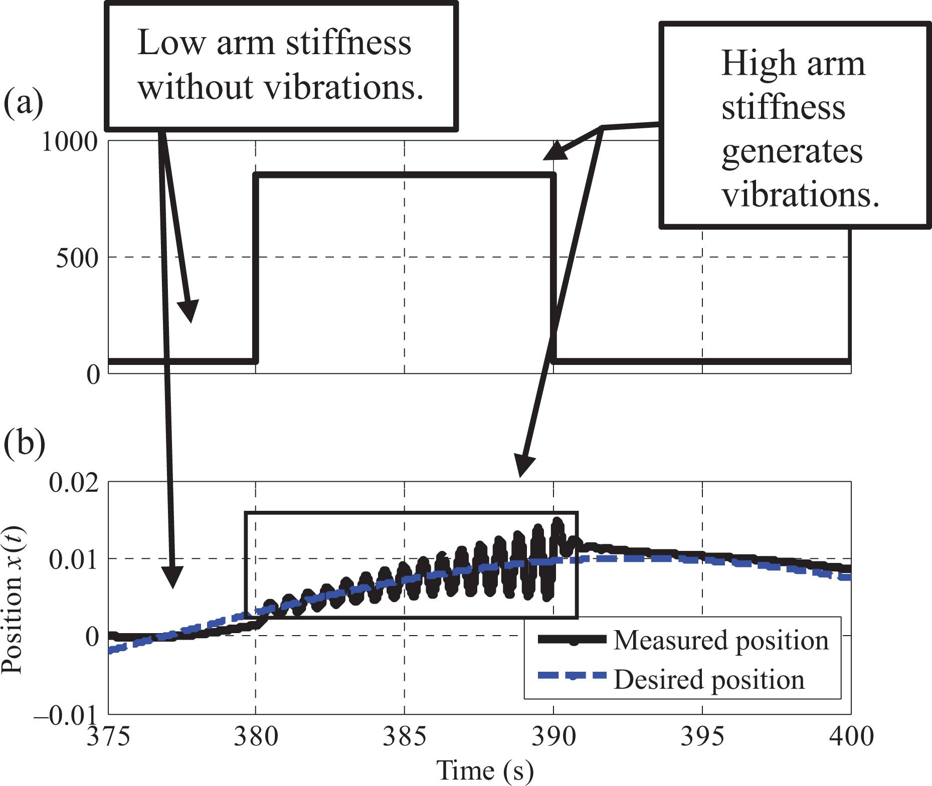
(a) The evolution of the human arm stiffness going from 50 to 850 in a square waveform and (b) the response of the suggested control loop without the observers.

Suggested control loop associated with the AVO. AVO: active vibration observer.
It should be emphasized that the following simulations are made with the 4-DOF IAD prototype (equation (7)). Hence, we will not use the velocity signal used in the previous sections but we will use other velocity signals v2 obtained from the simulations of the suggested control loop model, shown in Figures 3 and 15. These simulated velocity (v2) signals (SS; from the model in Figure 14) will be shown in the following sections.
Since the velocity signal has been changed, we should make some changes in the statistical analysis and the training of the ANN.
For the statistical analysis, all that we changed is the configuration of the ST-FFT and the analysis window. In fact, we changed the length of the aforementioned elements; they became a length of 500 samples, for the variance analysis, and 700 samples, for the standard deviation analysis. This increase of the windows length is coming from a decrease in the dynamic to measure since the inertia of the 4-DOF IAD model is higher than the 1-DOF reduced-scale robot. The results of this statistical analysis, when simulated with the SS, are presented in Figure 16(b) (i.e. the index of the variance observer, ISS) and Figure 17(b) (i.e. the index of the standard deviation observer, IS−SS). Regarding the training of the ANN, we used the same procedure explained in the section ANN but with some modifications. These modifications are explained as follows:
For this type of classification, a two-layer feedforward network with sigmoid hidden neurons and linear output neurons is created. This neural network is created with 10 neurons in the hidden layer and 1 neuron in the output layer, outputting a vector of a dimension 1 × 32 (i.e. the index IAVO−SS). Afterwards, this MLP was trained and tested with the SS represented in Figure 18(a). Its result is shown in Figure 18(b).
Accordingly, we built for each type of situation (i.e. vibrations-free situation and vibratory situation) 16 vectors corresponding to 16 segments of the velocity signal and each vector contains 300 values. Subsequently, we established a matrix P, for the training of the ANN, of a dimension 300 × 32 (i.e. combination of the 16 vectors corresponding to each type of situation).
The training of this ANN was performed with the same algorithm which is the Levenberg–Marquardt backpropagation algorithm.
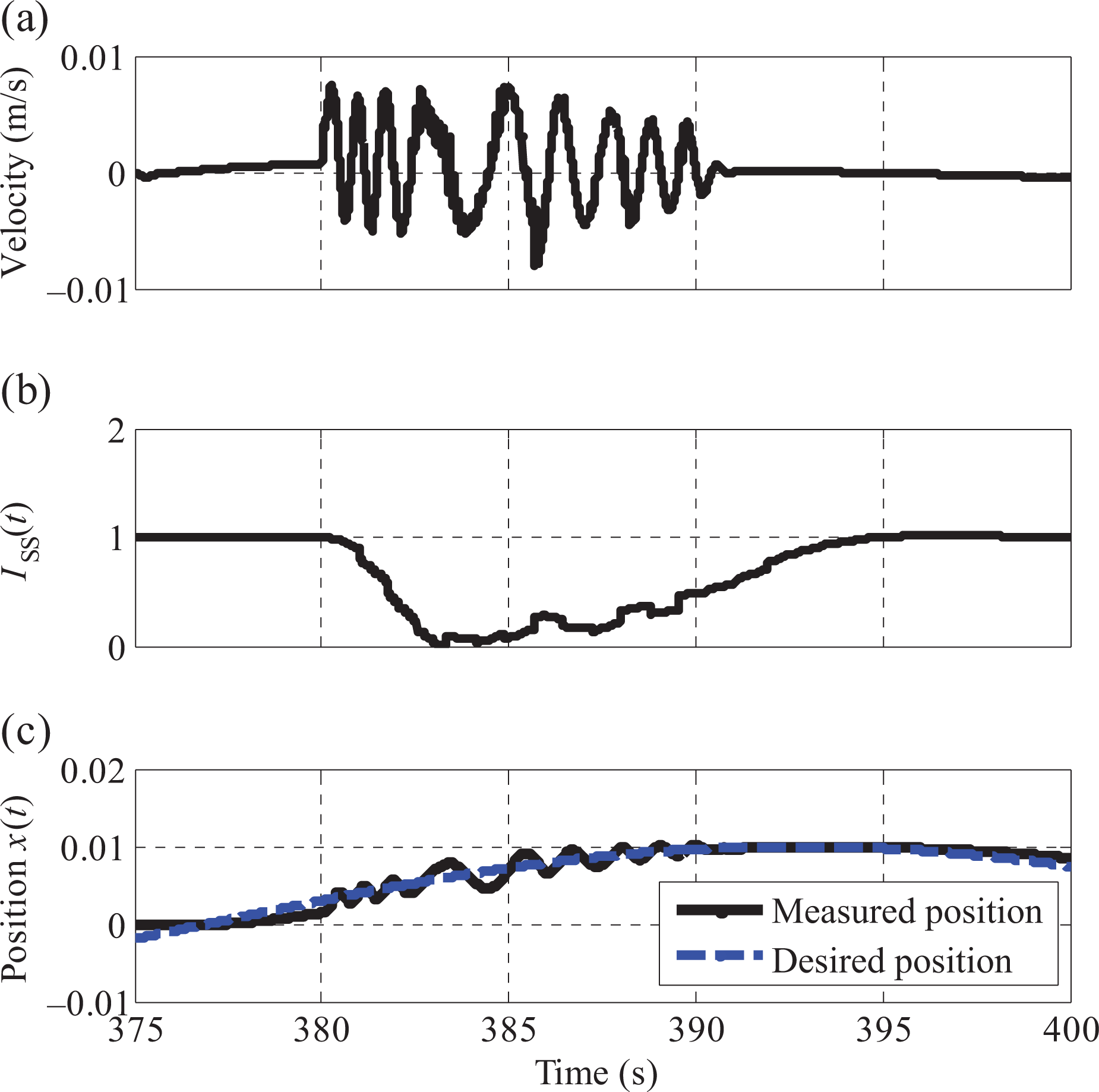
(a) The SS used as an input to the variance observer, (b) the evolution of the variance index in the time and the frequency domains and (c) the response of the suggested control loop when associated with ISS. SS: simulated velocity signal.

(a) The SS used as an input to the standard deviation observer, (b) the evolution of the standard deviation index in the time and the frequency domains and (c) the response of the suggested control loop when associated with IS−SS. SS: simulated velocity signal.

(a) The SS (v2) used as an input to the AVO, (b) the evolution of the AVO index labelled IAVO−SS and (c) the response of the suggested control loop when associated with IAVO−SS. AVO: active vibration observer; SS: simulated velocity signal.
Forthwith, after completing the necessary changes to accomplish the statistical analysis and the training of the ANN with the SS, we may set forth the analysis part of the experimental investigation.
Feedback using the AVO
The first experimental investigation was conducted in three parts.
The first part of the investigation is a simulation of the control loop without the suggested observers, as shown in Figure 4. This test was first made to help us verify the capability of our observers, especially the AVO, in ensuring safe and comfortable interactions. The result of this simulation is shown in Figure 14(b). In this figure, we can distinguish, very clearly, the vibratory behaviour caused by the human arm stiffness. In fact, we notice that an increase in the arm stiffness increases the vibration (in this figure, the behaviour is unstable: for a constant stiffness, the output increase). These results are consistent with the analysis presented previously and the results presented in the studies by Colgate and Hogan 7 and Duchaine and Gosselin. 9 In fact, based on the result shown in Figure 14(b), we can affirm that the human arm stiffness could destabilize the system. In our case, such vibrations are caused by the pole’s located at 10 rad/s illustrated by the resonance peak shown in Figure 8(d).
The second part of the investigation is a simulation of the suggested control loop associated with the AVO. The result of this simulation is presented in Figure 18(c).
The vibrations’ detection and reduction task by the AVO is performed as follows: The index IAVO−SS, shown in Figure 18(b), is used to properly update the proportional gain Kp according to the update rule given by equation (15). This proportional gain decreases while IAVO−SS approaches to zero (i.e. when the AVO detects the vibratory situation) for ensuring vibrations’ reduction in real time and then the stable interaction settles down. Thus, IAVO−SS increases to one (i.e. elimination of the vibrations: vibrations-free situation) and the proportional gain returns to its initial value (i.e. multiplication by one which is the value of the index when no vibratory behaviour is detected). Finally, the proportional gain’s update occurs in the same way whenever the AVO detects an unstable behaviour (i.e. a vibratory situation).
Finally, the third part of the investigation is a simulation of the suggested control loop associated with the AVO but when this latter is exposed to another velocity signal shown in Figure 19(b). This signal is resulting from a simulation of the closed loop when exposed to a force signal (with added noise), shown in Figure 19(a), as an input to the admittance model.
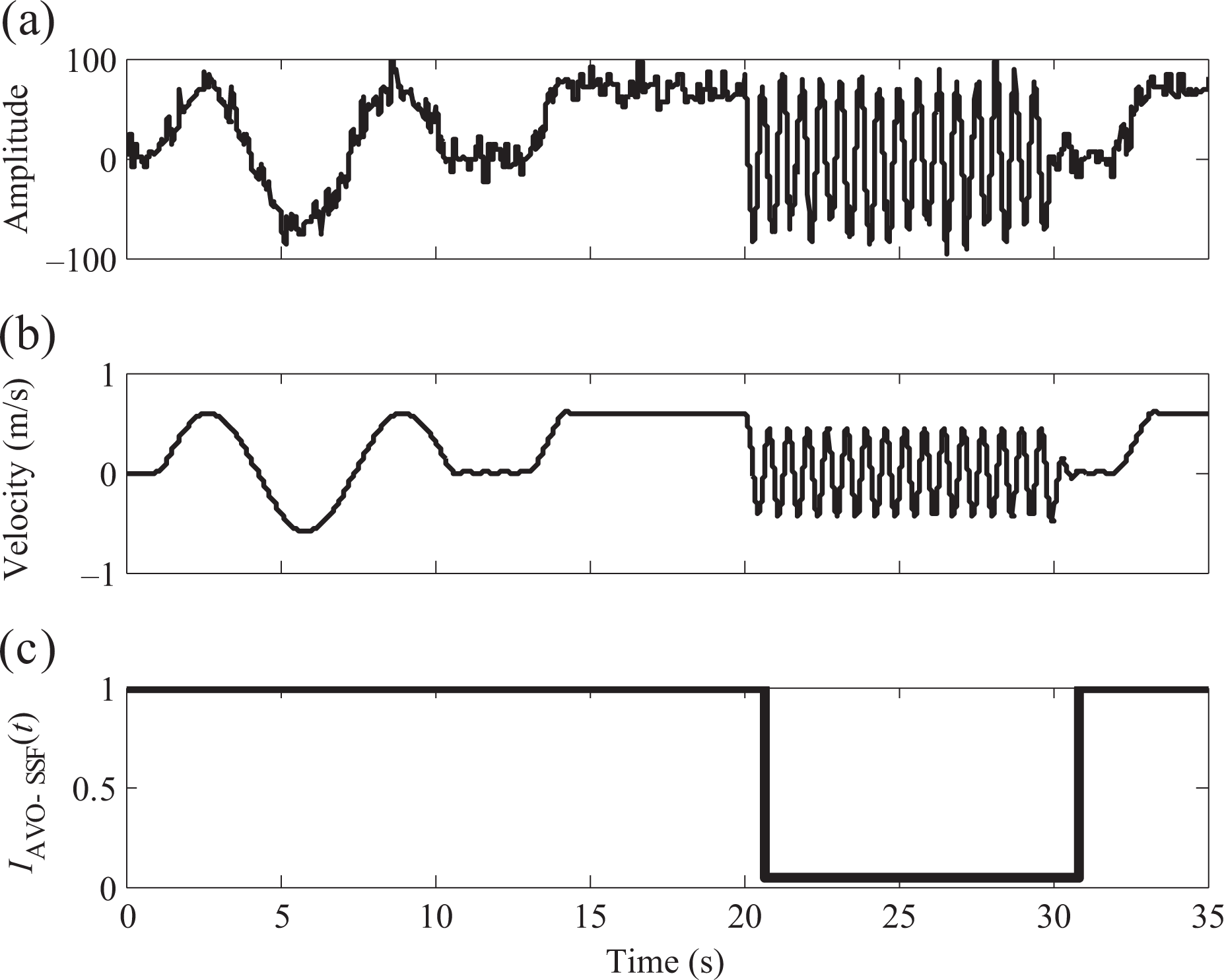
(a) The force signal used as an input to the admittance model with noise (noise power = 10, over the worst case), (b) the SS used as an input to the AVO and (c) the evolution of the AVO index labelled IAVO−SSF. AVO: active vibration observer; SS: simulated velocity signal.
To do so, we first begin by retraining the neural network with the SS. The training of the neural network was carried out with the same configuration of the previous neural network. Accordingly, our choice of the neural network was based on the minimization of the value of the MSE criterion. In fact, the smallest value of the MSE was found with an MLP having 10 neurons in the hidden layer, valued at 2.39952 × 10⁻²⁵. Such training results in an index IAVO−SSF shown in Figure 19(c).
The system response when associated with this index in closed loop is shown in Figure 20 where the solid black line represents the velocity response of the suggested control loop when associated with IAVO−SSF and the dashed blue line represents the velocity response of the suggested control loop without IAVO−SSF.

The response of the suggested control loop when associated with IAVO−SSF (solid black line) and the response of the suggested control loop without the AVO (dashed blue line). AVO: active vibration observer.
Based on this result, we may conclude that the AVO index IAVO−SSF is able to reduce the mechanical vibrations in the electric signal. Indeed, by comparing the velocity answer of the system when associated with this index (i.e. the solid black line) to the velocity answer of the system without this index (i.e. the dashed blue line), we notice a significant decrease in the vibrations.
Feedback using statistical analysis observer
We have replaced the index of the AVO in the closed loop by the index of the variance observer namely the index ISS, shown in Figure 16(b), in both the time and the frequency domains. The system response when associated with this index is shown in Figure 16(c).
Likewise, we want to assess the ability of the standard deviation observer in reducing the vibrations in pHRIs. Thereby, we have replaced the previous index by the index of the standard deviation observer, IS−SS, shown in Figure 17(b), in both the time and the frequency domains. The system response when associated with this index is shown in Figure 17(c).
Based on these responses, we can conclude that the indexes ISS (variance) and IS−SS (standard deviation) were able to reduce mechanical vibrations. Indeed, by comparing the answers of the system when associated with these two indexes to the system’s answer presented in Figure 14(b), we notice a significant decrease in the vibration amplitudes caused by an increase of the human arm stiffness.
Comparison with the TD-VOVC
For comparison purposes of our observers with other existing observers, the final experimental investigation was carried out with a different approach to those presented in this study. This approach, the TD-VOVC, is based on a detection of the mechanical vibrations present in the signal through an observation of the vibrations’ local maximums and minimums in the time domain. 33 To do so, we have replaced the indexes of our observers by the TD-VOVC index, shown in Figure 21(b). The response of the system when it is associated with this index is shown in Figure 21(c).

(a) The SS used as an input to the TD-VOVC analysis observer, (b) the evolution of the index generated with the TD-VOVC approach and (c) the response of the suggested control loop when associated with ITD-VOVC. SS: simulated velocity signal; TD-VOVC: time domain vibration observer vibration controller.
Discussion
The most effective way to avoid hindrance to human performance and to ensure safe and intuitive pHRIs is to detect and eliminate the sources of vibrations. In this sense, the suggested observer, AVO, gives some encouraging simulation results thanks to its ability in detecting and preventing the vibratory behaviours. In fact, it was found that the AVO is capable of detecting in real time the vibrations when they occur due to the existence of the operator arm stiffness in the closed loop. The AVO performs this detection while generating an index IAVO-SS when exposed to the SS shown in Figure 18(a) and an index IAVO-SSF when exposed to the SS shown in Figure 19(b). Indeed, when the vibrations are detected, the indexes tend to zero, otherwise they increase to one. Upon this, these indexes will be used in updating the proportional gain according to the aforementioned update rule (equation (15)), such that the gain introduced by the arm stiffness is cancelled by the AVO. Under this assumption, the loop gain becomes proportional to IAVO-SS and IAVO-SSF. When they decrease, the gain decreases for settling stable interactions by moving away the poles from the imaginary axis. Otherwise, they increase to one and the gain returns to its initial value when no unstable behaviour was detected (i.e. optimal operations).
Furthermore, the statistical analysis observer explained above, as well as the approach based on vibrations’ identification with references to local maximums and minimums (TD-VOVC), was also designed to reduce the mechanical vibrations distorting the operator’s safety and the robot’s stability and transparency but their performances were not enough for ensuring comfortable interactions.
Finally, since we have conducted several simulations with different approaches, one wants to know which one of them is the most appropriate for settling stable pHRIs. To do so, we have evaluated, for each approach, the robustness of the system by computing the error between the desired (x0) and the measured (x2) positions as shown in Figure 22.

The error (x2 − x0) evolution when the closed loop is associated with the AVO observer (a), with the variance observer (b), with the standard deviation observer (c) and with the TD-VOVC observer (d). AVO: active vibration observer; TD-VOVC: time domain vibration observer vibration controller.
By analysing Figure 22, we notice that the error between the desired and the measured positions, when the closed loop is associated with the AVO observer, is the one which has more tendency to converge to zero (i.e. minimization of the error) compared to the other errors (with lower frequency in the residual vibration).
In the following, further statistical analysis and performance analysis based on the execution times of each approach will be conducted to help us verify the validity of our algorithms and to affirm the aforementioned ascertainment. The statistical variable used in this investigation is the standard deviation performed in a period of time between 380 s and 390 s, exactly when the observers are activated (i.e. detection of a vibratory situation). The execution times will illustrate the time taken by each algorithm to perform a single treatment (i.e. one sample in the period of time between 380 s and 390 s). The results of these analyses are shown in Table 1, where the overhead presents the time taken to calculate all other blocks in the control loop (i.e. such as the IAD model, the human model, the admittance and the imperfections models) and the time taken to ensure the additions, the multiplications and the starting as well as the closing of Simulink.
Statistical and performance analyses results.

AVO: active vibration observer; TD-VOVC: time domain vibration observer vibration controller.
Based on these results, we notice that the lowest values of the statistical variable and the execution time, taken to perform a single treatment, are those obtained when the closed loop is associated with the AVO observer. From here, we may conclude that the AVO performs a better vibrations’ identification and reduction and thereby ensures more comfortable and more intuitive interactions. Hence, we can confirm that the AVO is the most appropriate approach for ensuring intuitive, safe and comfortable pHRIs. We still need to improve those results with an evaluation with human participants. However, since we know the threshold perception of humans to vibrations in the glabrous skin, 40 it would be possible to optimize the AVO under this threshold.
Conclusion
In order to ensure safe and intuitive pHRIs, vibratory behaviours should be detected and reduced under the human perception threshold. In fact, such behaviour could decrease the operations’ intuitiveness and robot’s transparency and could increase the operator’s safety risk. For that, two approaches have been presented for detecting and reducing the mechanical vibrations generated when collaborating with an IAD using an admittance control scheme. The first was a statistical analysis and the second was an MLP ANN. These approaches were designed in order to provide judicious indexes capable of ensuring an automatic update of the control loop gain as a function of the detected vibration amplitudes. Such adjustment could avoid hindrance to performance and intuitiveness in normal operations. Finally, based on our experimental results, we concluded that the AVO, based on an ANN approach, provided an accurate detection and reduction of the mechanical vibrations than the statistical analysis and the TD-VOVC approaches.
Future work will focus on an automatic optimization of the ANN in order to find an optimal solution for any mechanism, considering a multiobjective optimization. Of course, the stability could be achieved using other solution such as an elastic actuator 41 in order to control the equivalent stiffness of the human–robot interaction. Finally, a three-dimensional haptic virtual guide for satisfying better pHRIs in assembly tasks will be used for the evaluation of the technology with participants.
Footnotes
Declaration of conflicting interests
The author(s) declared no potential conflicts of interest with respect to the research, authorship, and/or publication of this article.
Funding
The author(s) disclosed receipt of the following financial support for the research, authorship, and/or publication of this article: This work is financially supported by the Fonds de recherche du Québec – Nature et technologies under the grant number 2016-PR-188869.