Sage Journals: Discover world-class research

Abstract

Automated guided vehicles require spatial representations of their working spaces in order to ensure safe navigation and carry out high-level tasks. Typically, these models are given by geometric maps. Even though these enable basic robotic navigation, they off-the-shelf lack the availability of task-dependent information required to provide services. This article presents a semantic mapping approach augmenting existing geometric representations. Our approach demonstrates the automatic annotation of map subspaces on the example of warehouse environments. The proposals of an object recognition system are integrated in a graph-based simultaneous localization and mapping framework and eventually propagated into a global map representation. Our system is experimentally evaluated in a typical warehouse consisting of common object classes expected for this type of environment. We discuss the novel achievements and motivate the contribution of semantic maps toward the operation of automated guided vehicles in the context of Industry 4.0.

Keywords

Semantic mapping AGVs object recognition SLAM

Introduction

Automated guided vehicles (AGVs) require spatial representations of their environment in order to enable autonomous navigation. Geometric maps are commonly used with occupancy grid maps being the state-of-the-art for robotic navigation. These enable basic robotic navigation, but they off-the-shelf lack the availability of environment-specific information. This article presents an approach to semantic mapping which augments common geometric representations by objects being relevant for logistic environments.

Navigation algorithms such as path planning or obstacle avoidance benefit from the additional knowledge about obstacles in the surrounding environment. For example, the presence of gates in warehouses might pose a problem for AGVs due to suddenly appearing humans, manually driven vehicles, or even other AGVs if there are no further communication systems available. Being aware of the presence of gates, algorithms are able to incorporate this which potentially results in a safer navigation.

Semantic maps provide a fundamental resource for AGVs operating as mobile service robots in logistic environments. In this way, they enable a vehicle to go, for example, to the «storage bin—12-02-01», «reloading point—5», or «charging station—7» with all positions being stored in the map.

Close-to-market systems solve this with the help of a human supervisor manually annotating maps or in rather exceptional cases using voice and gesture commands. The workload induced by this process is substantive, particularly for the initial setup of such a system. Thus the automatic annotation of such maps is appreciated for the introduction of AGVs in warehouses and is highly beneficial in the context of Industry 4.0.

Our approach aims at building semantic maps online while steering an AGV inside a warehouse (see Figure 1). This makes highly efficient object detection, simultaneous localization and mapping (SLAM), and map inference indispensable. The object detection utilizes efficient one-dimensional (1-D) segmentation over range as well as height information. These data are acquired through assumption of a 2.5-D world with end point of scans being described by a triplet of {x, y, h} with h being the height. The RGB-D images are segmented by means of discontinuities in the range and height data resulting in a set of regions of interest (ROIs) being considered for further processing. We observed that 2.5-D models are well suited for a multitude of man-made structures which specifically include logistic environments consisting of dominant vertical elements.

Figure 1.

An automated guided vehicle in a warehouse environment.

Our object recognition exploits the fact of a comparable limited object diversity being expected in warehouses. We therefore utilize geometric features covering physical dimensions of objects such as width and height. In addition to that, we investigate the visual appearance of object observations using a pre-trained deep convolutional neural network (DCNN/CNN) whose features are subsequently evaluated by a multi-class support vector machine (SVM). Our system is trained using solely publicly available image data and is evaluated in an environment it has never seen before. We expect the outcome to be highly beneficial since it allows to predict its overall ability to generalize from training data. The key contributions of this article can be summarized as follows:

a highly efficient segmentation and object detection based on 1-D contours;

a semantic mapping framework with near real-time performance;

integration of an SLAM framework for estimating globally consistent semantic annotations; and

experimental evaluation in an a priori unknown logistic environment.

Related work

The existing work in the area of semantic mapping can be categorized into different research fields in the computer vision and robotics communities and are further investigated as follows.

Deep learning and 2-D segmentation

The presence of DCNNs/CNNs significantly pushed the development in object and scene recognition. Based on the early work of LeCun et al. in the late 1980s,¹ there has been established a large number of algorithms such as the literature^2
–4 in the recent years utilizing CNNs. The baseline recognition performance has tremendously increased as, for example, compared to approaches based on SIFT and bag-of-words (BOWs) classification^5,6. In contrast to BOW-based approaches utilizing local features such as SIFT, CNNs use holistic images for feature extraction and classification. Out of the box, they are expected to be applied to images with the target object being centered and occupying the majority of the image. Prior image saliency estimation is required in order to make use of CNNs for analyzing images of complex scenes. In this line, a number of substantive work has been established, with selective search⁷ being a well-known representative. More recently, the novel methods of Edge Boxes⁸ and Bing⁹ have proven to be capable for real-time applications. All of these methods^7
–9 search the input image for ROIs being occupied by objects using different heuristics such as the responses of edge detectors.

Semantic scene understanding

The research field of semantic scene understanding has been investigated by the computer vision community. The availability of consumer-grade RGB-D cameras has essentially supported this. Silberman et al. proposed to segment RGB-D images into the classes such as floor, walls, and supportive elements and present an inference model describing physical interactions of these classes.¹⁰ Geiger et al. proposed a method for joint inference of 3-D objects and layout of indoor scenes.¹¹ Zheng et al. suggest a conditional random field (CRF) for dense segmentation and semantic labeling. Either of the methods provide powerful tools for semantic labeling achieving outstanding results. However, these implementations require a long computation time. The well-known real-time segmentation approach Stixel, proposed by Badino et al.,¹² has recently been extended by semantic labeling (Stixmantics¹³). The results reported for outdoor traffic scenes are surprising, moreover, with the real-time capability being achieved through the use of dense SIFT descriptors.

Object-based SLAM

In the recent years, the development of algorithms for visual simultaneous localization and mapping (V-SLAM) has essentially progressed. Thanks to the availability of graph-based optimization libraries such as g2o¹⁴ and iSAM,¹⁵ the application of V-SLAM for online operation is rendered possible. Several SLAM implementations utilizing these libraries were presented.^16–18 The state-of-the-art in SLAM focuses on the optimization of poses and landmarks which typically refer to local image features (e.g. SIFT¹⁹), geometric features (e.g. GLARE²⁰), ConvNet landmarks,²¹ or holistic image matching.²² There is only a small number of previous work utilizing semantic information in SLAM. Strasdat et al. presented SLAM++ which explicitly uses objects instead of landmarks.²³ Their approach is able to continuously track the camera pose while mapping objects in the surrounding environment. The authors mention that a re-localization based on object matching takes place once the tracking is lost. It is further emphasized that, thanks to object representations, the memory consumption is significantly reduced compared to dense geometric representations. The generic object pose estimation used in their work requires a GPU in order to enable close to real-time performance. Civera et al. presented a real-time mapping and loop-closure detection system with high performance omitting the use of GPUs.²⁴ The authors use SURF features quanitized inside a BOW approach for recognizing a priori learnt feature representations of objects which are incorporated in the map estimate. Due to the use of a monocular camera, the object poses are estimated by 2-D to 3-D feature correspondences and a perspective n-point algorithm.

Semantic mapping

Nüchter et al. proposed a semantic mapping approach that applies plane segmentation to 3-D laser data.²⁵ Though enabling high performance, it is restricted to planar regions. Stückler et al. presented an object-based extension for SLAM being able to generate dense 3-D object maps at a relatively high frame rate.²⁶ The authors utilize simple region features extracted from RGB and depth data to segment object regions from point clouds. The objects are classified using random decision forests and subsequently used to concurrently track the camera’s pose and estimate the 3-D poses of the objects. Even though, the approach is highly related to ours since the authors also make use of the geometric properties of objects in classification, we expect that the classification accuracy obtained with simple RGB region features can be substantially increased by CNNs. Grimmett et al. investigate the automatic mapping of parking spaces in garages based on lane marking detection in camera images.²⁷ Beinschob et al. present an approach for mapping logistic environments including the recognition of storage places and the automated generation of road map for AGVs.²⁸

Semantic place categorization

Semantic mapping in the context of labeling spatial subspaces with object categories has been investigated by several authors of the mobile robotics field. The early work of Mozos et al. extracts features from 2-D laser range data and trains Adaboost classifiers for distinguishing places of different categories. Pronobis et al. extended this by fusing data from 2-D laser range finders and cameras in an SVM-based place classification²⁹ which was extensively evaluated on a publicly available data set.³⁰ Hellbach et al. suggest the use of nonnegative matrix factorization (NMF) to automatically extract relevant features from occupancy grid maps which are subsequently utilized for identifying place categorizations.³¹ More recently, Sünderhauf et al. proposed an approach to semantic mapping using visual sensors.³² The authors make use of deep-learnt features extracted with a CNN which are passed to a random forest classifier. A continuous factor graph model is used to infer from the object observations. The area being covered by the camera’s field of view is labeled according to the output of the graphical model. The authors integrate their approach with state-of-the-art grid mapping solutions, such as GMapping³³ and Octomap,³⁴ in order to build geometric maps with the free space being supplemented by place category labels.

Summary

The computer vision research yields a number of high-level methods for feature extraction (CNNs), efficient segmentation, and semantic labeling. However, the use of solely 2-D image data for semantic labeling of holistic scenes entails the use of methods for generating region proposals. The measure of edgeness which is typically employed does not necessarily result in object proposals being expected or required which was also reported by Sunderhauf et al.³⁵ The missing depth data also hamper the use of scaled geometric object properties and height segmentation techniques. The existing methods for SLAM and semantic mapping either focus on the use of objects as landmarks²³ or are likely to provide fewer accuracy in large-scale object classification (36; 5) due to the image features being used. The related work in semantic mapping (2; 8) within the robotics community focuses on the extraction of one object class being of interest for investigated environment type (parking or storage spaces).

To our knowledge, there exists no prior work on online semantic mapping with the result of dense geometric maps with occupied space being assigned object labels with the accuracy of deep-learned models. Also, we expect the application of semantic mapping with recognition of multiple object classes in logistic environments to be novel in the robotics research.

Object recognition

The input RGB-D data of a camera are searched for objects. Thanks to the range data, the detection of occupied space in close proximity of the vehicle is simplified. A point cloud C is generated based on the input depth image. The architecture is visualized in Figure 2 and detailed in the following.

Figure 2.

Illustration of the architecture of our object recognition. The left part of the graph demonstrates the processing of the depth images and the right part the processing of the RGB images.

Ground plane segmentation

At first we filter those points of C reflecting the ground. The ground plane is estimated within the system calibration during a prior teach-in procedure. We therefore fit planes inside the point cloud computed based on the depth image and the calibration parameters. A RANSAC-based implementation for plane estimation of the library point cloud library (PCL)³⁶ is used for this step. The ground plane computed within the teach-in phase is kept fixed. We continuously check the validity of the ground plane to avoid mis-calibrations due to sensor relocations by forcing a minimum number of points being on the ground plane. For performance reasons, the continuous re-estimation of the ground plane is omitted which, thanks to fixed camera pose (w.r.t. the vehicle) and 2.5-D world constraints, provides accurate results. We define the remaining point cloud with the ground plane being removed as $\hat{C}$ .

Range and height scan

A top-down projection of $\hat{C}$ is generated by converting each point p ^(k) of $\hat{C}$ from Cartesian to polar coordinates as follows:

{(\begin{matrix} θ \\ ρ \\ h \end{matrix})}^{(k)} = (\begin{matrix} atan 2 (p_{y}^{(k)}, p_{x}^{(k)}) \\ \sqrt{{(p_{x}^{(k)})}^{2} + {(p_{y}^{(k)})}^{2} + {(p_{z}^{(k)})}^{2}} \\ p_{z}^{(k)} \end{matrix})

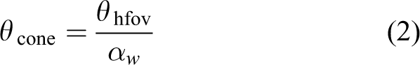
where θ ^(k) refers to the bearing, h ^(k) to the height over ground, and ρ ^(k) to the range of the point k relative to the camera origin. We further introduce θ _hfov as the entire camera’s horizontal field of view and θ _cone as the width of one measurement cone. Either of the parameters can be estimated straightforward based on camera calibration parameters. Given the horizontal field of view of the camera θ _hfov and the image sensor’s resolution α_w , we calculate the width of one measurement cone as follows

θ_{cone} = \frac{θ_{hfov}}{α_{w}}

Depending on the depth measuring sensor used and the resulting density of the obtained point cloud, it is recommendable to either exclude cones without depth values or interpolate the depth data with a Gaussian kernel around these locations.

Let us assume that $θ_{hfov, b}^{-}$ and $θ_{hfov, b}^{+}$ refer to the boundaries of the measurement cone b. Then a vector of point indices s with the minimal values s(b) can be calculated as follows

s (b) = min_{θ_{hfov, b}^{-} \leq θ^{(l)} < θ_{hfov, b}^{+}} (ρ^{(l)}), l \in \hat{C}

In this way, we obtain the contour s(b) consisting of points with each being closest to the camera origin inside a cone b.

Curvature detection

In order to detect objects, s(b) is further analyzed. The physical boundaries of objects in the world typically entail notable changes in curvature. We exploit this property to enable an efficient object detection based on features extracted from a 1-D contour. We shift the signal s(b) by a constant offset w resulting in $\hat{s} (b)$

\hat{s} (b) = s (b) - s (b - w)

for (b − w) > 0. The difference signal $\hat{s} (b)$ is used to identify peaks in the curvature given a minimum threshold λ_ds

e^{+} = {\hat{s} (b - 1) > λ_{d s}}

e^{-} = {\hat{s} (b) < - λ_{d s}}

with e ⁺ and e ⁻ denoting peaks originated from positive and negatives slopes, respectively. It is necessary to distinguish this case instead of incorporating the absolute values in order to locate the peaks correctly.

Segment estimation

Having obtained the putative object boundaries E = {e ⁺ ∪ e ⁻}, we utilize the consecutive peaks E_i and E _i+1 to identify subsets of the contour corresponding to objects in the world. The width w(i) and the height h(i)* for each subset i are obtained as follows

h (i) * = median [h (E_{i},..., E_{i + 1})]

w (i) = \sqrt{{(p_{x}^{(E_{i})} - p_{x}^{(E_{i + 1})})}^{2} + {(p_{y}^{(E_{i})} - p_{y}^{(E_{i + 1})})}^{2}}

The object proposal O_i consisting of the segment data {w, h}_i is forwarded and evaluated by the object retrieval.

Object retrieval

The object observations are defined by the segments O = {o ₁, o ₂, ..., o_n }] with o_i = (w, h)_i being its associated property vector. The prior object database is searched for corresponding items based on o_i . We use a KD-tree with approximate nearest neighbor search constructed based on dimensions being commonly observed for particular object classes P = {p ₁, p ₂, ..., p_n }. The database consists of n entries with p_i = (w, h, c)_{_i} describing object properties of the class c. The object retrieval implements the nearest neighbor search NN(o_i , P) ∈ P given the query o_i ∈ O and a distance metric dist

NN (o_{i}, P) = \underset{p \in P}{argmin} dist (o_{i}, p)

The estimated height and width of an object are subject to uncertainties due to the range-dependent measurement accuracy of RGB-D sensors. We account for this by introducing the following covariance matrix M

M = (\begin{matrix} 0.5 m_{w} m_{r} & 0 \\ 0 & 0.1 m_{h} m_{r} \end{matrix})

with m_w , m_h , and m_r being individual weights for the width, height, and range uncertainties, respectively. Both, width and height, are equally affected by the range uncertainty being modeled by m_r . The factor m_w is set according to the position of the object in the image coordinate frame. This addresses the problem of detections close to the image boundaries resulting in partial object observations. A similar effect can be observed for large objects being close to the image sensor. The constant factors 0.1 (for height) and 0.5 (for width) are added to the covariance estimation in order to account for object occlusions which can occur anywhere in the image and hence are hard to estimate online. Since occlusions rather affect the width estimation of an object, the height provides a more certain contribution to the object class retrieval

m_{w} = 1 + {\begin{matrix} p_{x} (E_{i}) < γ_{x, min} & e^{- \frac{1}{2} \frac{{(p_{x} (E_{i}) - μ_{w, min})}^{2}}{σ_{w}^{2}}} \\ p_{x} (E_{i + 1}) > γ_{x, max} & e^{- \frac{1}{2} \frac{{(p_{x} (E_{i + 1}) - μ_{w, max})}^{2}}{σ_{w}^{2}}} \\ otherwise & 0 \end{matrix}

m_{h} = 1 + {\begin{matrix} p_{y} (h_{i}) < γ_{y, min} & e^{- \frac{1}{2} \frac{{(p_{y} (h_{i}) - μ_{h})}^{2}}{σ_{h}^{2}}} \\ otherwise & 0 \end{matrix}

m_{r} = e^{- \frac{1}{2} \frac{{(r_{i - μ_{r}})}^{2}}{σ_{r}^{2}}}

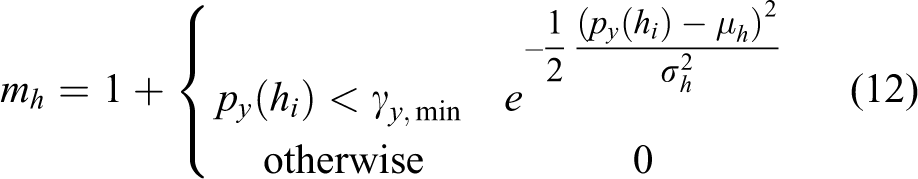
The weighting factors m_w and m_h can be interpreted as a Gaussian filter applied to the boundaries of an image. The closer an object approaches the image boundaries, the more uncertain is the estimation of its width and height. This weighting filter can be efficiently implemented using a pre-calculated lookup table. The parameter σ_r is set according to the properties of the range sensor. The Mahalanobis distance is utilized to incorporate the presented observation uncertainty within the nearest neighbor search of equation (9) which is defined as

dist (o_{i}, p, C_{i}) = ((o_{i} - p) C_{i}^{- 1} (o_{i} - p {))}^{1 / 2}, p \in P

As a result of this step, we obtain a set of object class proposals $\hat{O}$ matching our database descriptions P based on the object observations O. These proposals are further investigated by means of RGB features which are described in the following.

ROI estimation

The object proposal ${\hat{O}}_{i}$ with the associated properties {w, h}_i and contour boundaries (E_i , E _i+1) is prepared for further appearance-based analysis. A bounding box around the object is generated as ROI inside the RGB image. We therefore transform the object proposal $\hat{O}$ into the coordinate frame of the RGB camera based on the properties ${w, h, p_{x} (E_{i}), p_{x} (E_{i + 1}), p_{y} (E_{i}), p_{y} (E_{i + 1})}$ . Subsequently, the image content of the ROI is passed to the CNN-based feature extraction.

CNN features

This processing unit extracts features from the RGB image data. This process is restricted to the areas defined by the ROIs of the prior detection step. For this purpose, we use a CNN. The principle of CNNs can be summarized as follows. A set of convolutional filters are repeatedly applied to the 2-D image data. The filters’ outputs are collected into nonoverlapping grids. The next layer subsamples the input data by applying pooling methods such as taking the maximum or average of the grid. The combination of convolving and subsampling the input data is repeatedly carried out at successive network layers. This method allows to learn features at different scales and spatial positions in the image. The complex fully connected layers of neural networks are typically found at the end of a CNN. The outputs of different CNN layers can be combined for the final output. The CNNs differ significantly from other feature extraction methods used in computer vision since they learn features and their distributions at different levels (e.g. parts, objects, and local characteristics) given the training data. Depending on the depth, the layers respond to different scales of an object. The further a layer is located from the input layer, the more local will be the response and the smaller the affected area of a firing neuron. As a feature extractor, we make use of the pre-trained CNN CaffeNet ³⁷ which consists of seven layers with our system utilizing the fc7-layer. Since this layer is located at the end of the network, we obtain a 4096-dimensional feature vector capturing local image characteristics.

Image/ROI classification

The content of each detected object is classified based on the ConvNet features extracted within its ROI. This procedure is applied to dynamic objects such as pallets, forklifts, and humans. In addition to those, we classify the feature vectors generated from the entire image in order to detect larger objects such as gates and racks. We train a multi-class SVM following a one-versus-all schema. Hence, we train one binary SVM for each class i

b_{i} \cdot (w_{i}^{T} \cdot x_{i} + w_{i, 0}) \geq 1

We use a linear kernel which can be defined as the following cost function:

Ψ (w_{i}) = \frac{1}{2} w_{i}^{T} w_{i}

We observed that using a linear kernel provides promising classification results while keeping the computational costs at a minimum. This is necessary since a more complex system has to evaluate a large number of classifiers for each obstacle being detected at a high frequency. Each SVM is trained with positive samples of one target class and negative samples being randomly drawn from the other classes as well as images describing various objects not being recognized by our system such as walls, ladders, and windows. We use one set of binary SVMs for dynamic (ROI) and another set for static objects (entire image). It is possible to recognize multiple dynamic and one static object in a single image, for example, pallets placed inside a rack. The ROIs and images being evaluated are labeled with the class having the minimum distance to the input feature vector. Those object proposals exceeding a distance threshold τ _svm are labeled as unknown. The combination of SVMs and CNNs provides a number of advantages compared to soft-max layers being typically placed at the end of a CNN for classification. First, the performance of this layer is reliant on preceding network layers which is why they are typically reconfigured as well. Training a CNN is computationally expensive and requires a large appropriate set of training images in order to enable reasonable generalization performance. Solely continuing the training of the soft-max layer is indeed possible but to our experience performs worse than SVMs which was also shown in Huang and LeCun.³⁸ Second, we also found that combining SVMs with CNNs enables a straightforward adaption to other application scenarios, since training SVMs with input features of a static CNN can be accomplished with reasonable effort.

Range scan annotation

The range scan s being generated in the previous steps is fused with the detected object proposals. Each cone s(b) is assigned the corresponding class label. Those not being described by a known object class are assigned the label unknown. If an object was detected for the entire image, we assign each measurement having a range ρ below ρ _max the estimated class label. This annotated range scan provides the fundamental for our semantic mapping algorithm.

Semantic mapping

The integration of our semantic mapping algorithm is illustrated in Figure 3 and described in depth in the following section.

Figure 3.

Overview of our semantic mapping system with its components and their data flows.

Integration of object proposals in pose graph SLAM

Pose graph SLAM: Providing the navigation of a mobile robot is carried out in a 2-D space, its state vector can be described by x = (x, y, ϕ)^T. Pose graph SLAM optimizes robot poses x_i of a given trajectory. The graph consists of vertices given by the poses x_i and edges between the poses x_i and x_j. The action u_i = Δ(x, y, ϕ) is carried out in order to get from the state x_i to x_i+1 and is incorporated according to a motional model

x_{i + 1} \sim N (f (x_{i}, u_{i}), Σ_{i})

Without loss of generality, we can describe the motion of loop closings detected for the poses x_i and x_j by u_ij, hence we can postulate the following state x_j

x_{j} \sim N (f (x_{i}, u_{i j}), Λ_{i j})

Given all states X and all actions U, we aim at finding the maximum a posteriori estimate of robot poses X ^* for the joint probability distribution

X^{*} = \underset{X}{argmax} P (X | U)

We can account this by the following factorization

P (X | U) \propto \prod P (x_{i + 1} | x_{i}, u_{i}) \cdot \prod_{i j} P (x_{j} | x_{i}, u_{i j})

with P(x _i+1|x_i ,u_i ) expressing odometry constraints and P(x_j |x_i ,u_ij ) the loop closure constraints. We can express the objective function (equation (19)) as a nonlinear least squares optimization problem that can be solved using Gauss–Newton

X^{*} = \underset{X}{argmin} \sum_{i} {‖ e_{i}^{odo} ‖}_{\sum_{i}}^{2} + \sum_{i j} {‖ e_{i j}^{lc} ‖}_{Λ_{i j}}^{2}

with $e_{i}^{odo} = f (x_{i}, u_{i}) - x_{i + 1}$ and $e_{i j}^{lc} = f (x_{i}, u_{i j}) - x_{j}$ . An extensive derivation of this is given by Sünderhauf and Protzel.³⁹

Object proposals: Our approach optimizes a pose graph given the odometry and loop closure constraints as shown in equation (21). We continuously detect objects which are incorporated during the mapping process. Each object detection O _i* is linked to a reference pose x_i and associated with a set of measurement points representing the object. The reference poses are continuously updated during the graph optimization. The resulting differences of the poses typically occur as a result of loop closures and when, for example, re-traversing longer trajectory paths from the opposite direction. These changes have to be taken into account for referencing the detected objects with respect to the pose graph and eventually the global map. The object points O _i* are kept in the coordinate frame of the corresponding pose x_i. For higher level layers of our semantic mapping framework, we frequently transform the object points into the global coordinate frame of the map with the origin being centered at the first SLAM pose x ₁.

Even though it is generally possible to include the object points in the graph optimization, similar to our previously presented approach¹⁶. This additional optimization is quite expensive and hence might entail a significant performance loss for online mapping.

Probabilistic grid mapping with semantic information

This section explains our method for transferring a graph-based map structure into a global semantic grid map. First, we will introduce how a regular spatial structure is generated and the object observations are transferred. The subsequent inference on the initial estimate of the map will be discussed.

From a pose graph to a semantic grid map: Given an optimized graph with poses X* constructed as described in the ection “Integration of object proposals in pose graph SLAM ,” all points o_i associated with the pose x_i are transformed into a global map reference which results in a transformed set of points o_i*. We define m as our map with m_j representing a grid cell. The (x, y)-coordinates of the center-of-mass of m_j are expressed by m_j,x and m_j,y , respectively. The transformation of each point $o_{i}^{(k)}$ into the map coordinate frame is carried out as follows

(\begin{matrix} m_{j, x} \\ m_{j, y} \end{matrix}) = ⌊ [(\begin{matrix} o_{i, x}^{(k)} \\ o_{i, y}^{(k)} \end{matrix}) - (\begin{matrix} c_{x} \\ c_{y} \end{matrix})] τ^{- 1} + \frac{1}{2} (\begin{matrix} s_{x} \\ s_{y} \end{matrix}) ⌋

where S_x and S_y refer to the size of the entire grid map, c_x and c_y to the origin of the map, and τ to the grid resolution. The origin c of the map is defined by the first pose of the SLAM graph, thus c = x₁. The grid resolution τ _res has to be set appropriately and suit the underlying RGB-D sensor characteristics.

Each grid cell m_j consists of a probability distribution p(m_j ) with each element describing one object class. Having estimated the corresponding grid cell m_j for each point $o_{i}^{(k)}$ , we are able to update p(m_j ) for m_j given our observations $p (o_{i}^{(k)})$ . Note that for occupancy grid maps, m_j denotes one occupancy probability, whereas m_j in our approach describes a discrete probability distribution of object affiliations. The states unknown, occupied, and free can be inferred from our p(m_j ) though. Each distribution p(m_j ) is estimated by those points of O* that end inside m_j according to equation (22). We define this subset of O* as O_j *.

p (m_{j}) = η \sum_{k} p (o^{(k)}), k \in O_{j}

where η denotes a normalization factor. The initial state of each m_j is a uniform distribution.

Our approach implements an end point model with each measurement point being directly assigned to the corresponding grid cell omitting cells inside the ray’s cone. This is necessary in order to ensure an efficient map update. A number of robotic navigation tasks such as path planning often require more comprehensive environment descriptions which explicitly consider free space. For performance reasons, we avoid expensive ray-casting models accompanied with this and suggest building those subsequently or in parallel but slightly delayed.

Since the map size and the number of object likelihoods stored in the cells easily increase in large-scale environments, it is recommended to use sparse instead of dense matrices. Particularly, high-resolution maps usually encode a lot of free space. The point transformations being applied frequently are highly optimized thanks to efficient matrix operations.

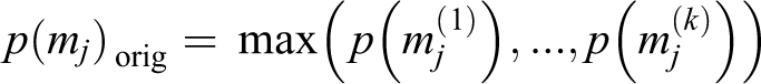
Inference: The initial estimate of the semantic map m typically consists of uncertainties which can occur due to the following reasons. Accumulated errors of the pose estimation might remain after the pose graph optimization if the distance traveled by the robot from the last loop closure is too long which is why errors cannot be adequately corrected. This effect can potentially be noticed in path segments at the end of a trajectory which results in object detections being incorrectly assigned to spatial grid cells m_j . In addition to that, the map estimate is induced by uncertainties in the object recognition due to the detections of multiple object classes. This effect can be observed more frequently, particularly in the presence of object classes of similar visual appearance and geometric properties as, for instance, wall and gate. It affects the distributions of object affiliations p(m), rather than the spatial positions of m. Uncertainties due to this reason are not just a drawback: they also allow to identify false-positive object detections based on multiple observations, potentially originated from varying perspectives or different path segments.

Due to the abovementioned reasons, it is necessary to explicitly account for the uncertainties in the semantic map estimation. For this purpose, we make use of the Shannon entropy which is separately estimated for each grid cell as follows

H (m_{j}) = \sum_{k} p (m_{j}^{(k)}) log (\frac{1}{p (m_{j}^{(k)})})

The Shannon entropy provides a beneficial measure of uncertainty as revealed by the probability distributions of the semantic grid cells. The measures of H(m_j ) are utilized to infer the final class label from p(m_j ). Providing a value of H(m_j ) < λ _max, we set the final label of m_j * to the label with the highest probability as follows

p {(m_{j})}_{orig} = max (p (m_{j}^{(1)}),..., p (m_{j}^{(k)}))

p {(m_{j})}_{surf} = max (p (m_{j, surf}^{(1)}),..., p (m_{j, surf}^{(k)}))

p (m_{j} *) = {\begin{matrix} H (m_{j}) > λ_{high} & p {(m_{j})}_{orig} \\ λ_{low} \leq H (m_{j}) \leq λ_{high} & p {(m_{j})}_{surf} \\ H (m_{j}) < λ_{low} & p (c l_{unknown}) \end{matrix}

p (m_{j, surf}) = η \sum p (m_{k}), k \in m_{j, surf}

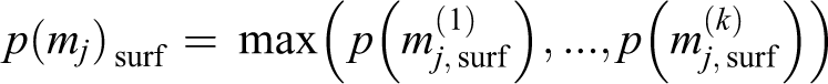
The differentiation of high-, low-, and unconfident estimates is required to ensure robust class label assignments. Those cells possessing an entropy measure H(m_j ) below the threshold λ _low are directly assigned the class label unknown. For low-confident estimates with values in the range of λ _low and λ _high are considered for further investigation. We therefore analyze adjacent cells of m_j sharing the same surface entity. The crux here is that we do not incorporate all adjacent grid cells of m_j , but those that are likely originated from the same physical object in the world based on height and surface constraints.

Semantic grid cells providing a high confidence H(m_j ) are directly adopted omitting the consideration of adjacent cells. This is done in order to avoid confusions and thus of the distribution p(m_j ) which can, for example, occur when small objects such as rack poles contributing to only a single or a low number of grid cells. The object labels of those are risked to be filtered out if it is merged with a potentially diverse neighborhood.

The presented method enables efficient inference of final class labels m_j * for each entity of the semantic map. Technically, it is possible to store the probability distribution m_j . However, this requires a large amount of memory for large-scale environments and increasing numbers of object classes. We further expect that the majority of applications utilizing semantic maps needs direct knowledge about the underlying object classes, rather than a distribution of object likelihoods. In order to incorporate the uncertainty in the class estimate, it is recommended to store the entropy values H(m) along with m_j *.

Experiments

This section presents the experimental results obtained using the object recognition and semantic mapping algorithms as explained earlier in this article. We will describe the experimental setup and the results for each component of the system, in particular the segmentation, classification, and the semantic map generation.

Setup

We evaluate the presented approach by experiments carried out in a warehouse which consists of a multitude of common objects expected for this type of environment. The data are collected with a reach truck which has been fully automated for a research project. For the purpose of generating a semantic map, we manually steered the vehicle inside the warehouse. The RGB-D image data utilized by our system are recorded using an Asus Xtion camera which is aligned sideward with respect to the vehicle’s direction of travel. We use the following parameters in our experiments: θ _hfov = 1.012 rad, α_h = 640 px, ρ _max = 5.0 m, w = 4, λ _ds = 0.09 m, μ_r = 0 m, μ_h = 3.36 px, μ _{w, min} = 3.36 px, μ _{w, max} = 636.69 px, γ _{x, max} = 560 px, γ _{y, min} = 80, γ _{x, min} = 80 px, σ_w = 31.05 px, σ_h = 31.05 px, σ_r = 2.0 m, τ _svm = 0.4, and τ _res = 0.05 m.

Segmentation

This experiment analyzes the performance of the object detection system before the retrieval and classification components. We therefore run the detection and store the input RGB images along with the overlayed bounding boxes. The amount of correct, incorrect, and missing detections is determined irrespective of the actual class labeling. Thresholds and parameters of the segmentation are kept fixed. We obtain an overall detection rate of about 87.21%.

Classification

We further evaluated the classification accuracy achieved based on the object retrieval priors and the appearance-based classifier. Table 1 provides details about the training phases of the SVMs including iterations, number of support vectors, and amount of training images. As already mentioned, we make use of a set of 500 negative training samples capturing objects not being recognized by our system. From this set, we randomly sample about 150 images and another 150 samples are selected from the training images of the other object classes. The data set is split into 50% training and 50% testing images. The entire training and testing data set is obtained from publicly available image sources being supplemented by our own image collection. These images are edited in the way such that only the object of interest is visible. We captured an additional validation data set consisting of RGB and depth images in the mentioned warehouse. The ground truth for the validation data set is obtained by manually labeling the input RGB images. We assume that at least 50% of an object of interest has to be visible in order to assign an image the corresponding class label. This addresses the classification of entire images (for gates and racks) as well as the ROI-based classification of objects such as forklifts, pallets, and humans. The object segmentation expects this amount in order to minimize false-positive detections while simultaneously enabling as many as possible recognitions of objects in the presence of clutter and close to the image boundaries. The results are shown in Figure 4 and Table 2. The values of the ROC curves are obtained by varying distance thresholds τ _svm of the SVM classification. Note that none of the training and testing images was captured in the warehouse used for the validation.

Table 1.

Details of the training phase: number of training, testing, and validation images; training iterations; number of support vectors; and area under the curve values on testing data are shown for each class.

Class	# Images			Iteration	# Support vector	AUC
Class	Train	Test	Validation	Iteration	# Support vector	Test
Forklift	288	288	—	352	148	0.995
Human	186	186	—	271	120	0.991
Pallet	139	139	652	289	125	0.992
Rack	108	108	904	288	109	0.989
Gate	122	122	365	392	114	0.981

AUC: area under the curve.

Figure 4.

ROC curves for all object classes captured on the validation data set. The figures show the results of the prior training (red) and the ones of the validation (blue). ROC curve for object class (a) pallet, (b) Rack, (c) Gate.

Table 2.

Results of the SVM-based classification with priors obtained from the object retrieval.^a

		Bounding box		Obstacle type
Class	AUC	ROI	Image	Dynamic	Static
Pallet	0.984	X		X
Rack	0.852		X		X
Gate	0.961		X		X

SVM: support vector machine; ROI: region of interest; AUC: area under the curve.

^aThe table provides the AUC, the corresponding evaluation window, and the obstacle type.

SLAM

Our graph-based SLAM poses the fundamental for the spatial mapping of objects and the estimation of the vehicle’s pose with respect to the environment. There have been proposed a number of metrics for benchmarking algorithms as, for example, those introduced by the Rawseeds project.⁴⁰ The ground truth is obtained using a laser range finder and the algorithms described by Himstedt et al. ¹⁶ The accuracy of the estimated trajectory is expected to be below 0.04 m, thanks to the high measurement accuracy of the laser range finder and a joint map and pose refinement.¹⁶ The results of the presented camera-based SLAM approach are compared to the ground truth based on the absolute trajectory error (ATE).⁴⁰ The mean error is 0.26 m in the position and about 0.07 rad in the orientation, respectively.

Semantic labeling

In addition to the evaluation of the accuracy of our SLAM framework, we investigated the key contribution of this article which is the semantic annotation of the occupancy grid map. Our ground truth is generated by manually labeling the grid cells of our prior map provided by the SLAM algorithm. The evaluation of the semantic annotation is carried out by comparing the ground truth to those being obtained initially (unoptimized) and those being optimized. The results are visualized in Figure 5 and summarized in Table 3.

Figure 5.

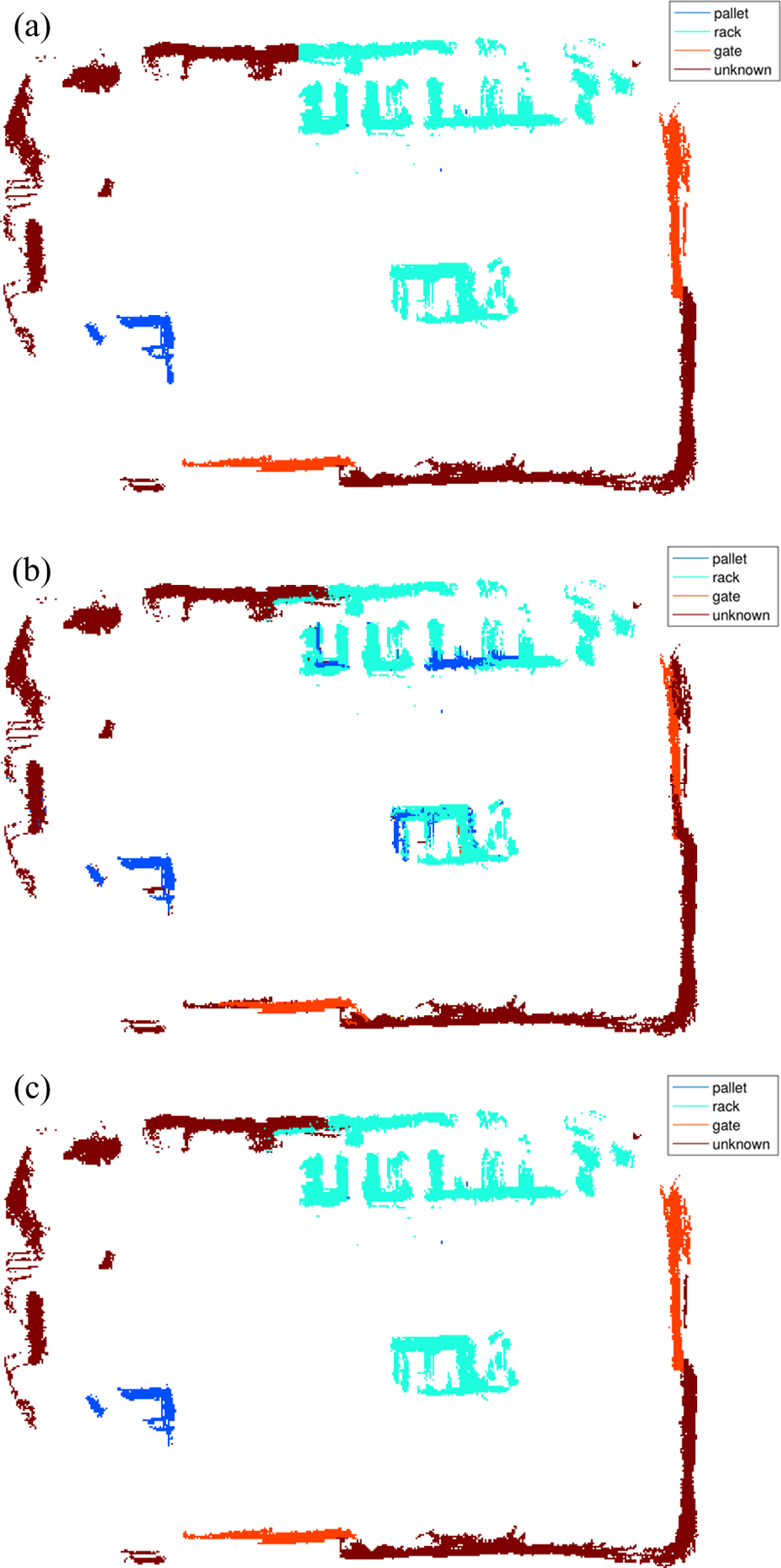
The figures demonstrate our experimental results obtained in warehouse environment. The ground truth labels are obtained by manually annotating all non-empty grid cells. (a) Semantic map with ground truth labels. (b) Initial semantic labels without optimization. (c) Initial semantic labels with optimization based on uncertainty estimation and incorporating adjacent cells.

Table 3.

Semantic labeling results.

Method	# Matching labels	Accuracy
Unoptimized labeling	10310/11278	0.914
Optimized labeling	11021/11278	0.977

Performance

In our experiments, we used a Dell Latitude E6320 laptop equipped with an Intel Core i7 dual-core processor and 8 GB RAM. The processing time required by each system component is detailed in Table 4. Our system runs at about 4 Hz in the mean and never drops below 2 Hz. Note that some of the components do not necessarily have to run all the time, for example, the occupancy grid map can be re-estimated at a much lower rate or can even be done only once at the end of the trajectory. The semantic map is estimated independently of the occupancy grid map and requires significantly less computation time due to the end point model being utilized instead of expensive ray casting. Also the rates of the loop-closure detection and graph optimization can be reduced to, for example, 0.5 Hz. Based on these simplifications and extensive use of parallel programming, we observed de facto run times of about 5–10 Hz.

Table 4.

Performance of our system and individual components.

Component	Time (ms)
Component	Mean	Max
Object recognition	162.85	269.07
Ground plane estimation	162.85	17.19
Range scan generation	9.53	9.88
Height scan generation	5.12	6.31
Curvature detection	0.31	0.4
Segment estimation	10.86	19.2
Object retrieval	0.91	1.74
ROI estimation	23.09	24.11
CNN feature extraction	73.49	156.09
Image/ROI classification	18.81	29.67
Non-max suppression	2.11	2.55
Range scan annotation	1.71	1.93
SLAM	85.07	176.66
Loop closure detection	23.44	37.89
Graph optimization	22.35	52.8
Occupancy grid mapping	39.28	85.97
Semantic annotation	25.32	57.07
Object point transformation	3.45	3.67
Label assignment	8.91	9.86
Inference	12.96	14.22
Total	273.24	498.8

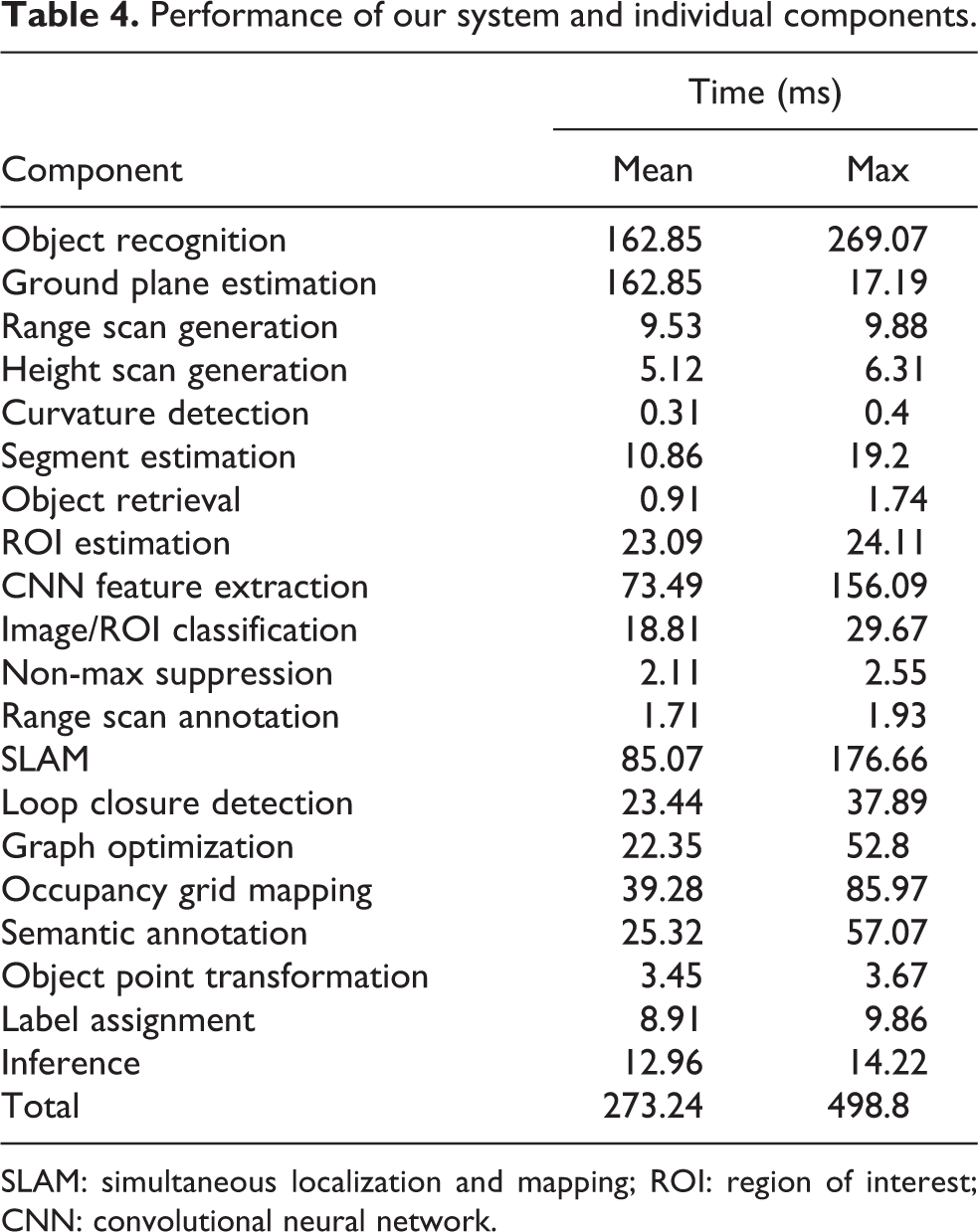
SLAM: simultaneous localization and mapping; ROI: region of interest; CNN: convolutional neural network.

Discussion

Our object segmentation and retrieval provides an efficient solution for online semantic mapping. The classification results obtained for the validation data set demonstrate the high generalization performance of the CNN and SVM. This becomes particularly obvious since the appearance of many objects on the training images differs from those in the testing warehouse. The detection of pallets and gates is outstanding, the one for racks is slightly worse. We expect that this is due to the fact that our training data mainly consist of racks being fully equipped with pallets which are not the case for all racks in our testing environment. Thanks to the descriptive power of the CNN features, we are able to achieve a high classification accuracy for SVMs with linear kernels given a relatively small amount of training data, especially compared to approaches based on HOG features.⁴¹ The CNN features in combination with observations of multiple viewpoints being correctly referenced by our SLAM algorithm enable the correct labeling of more than 97% of the grid cells.

Conclusion

We introduced a solution for semantic mapping of logistic environments. Our prior segmentation enables to efficiently generate object proposals by exploiting geometric properties of objects being observed in a scene. These geometric features are fused with textural properties of objects which are extracted based on deep-learned features from a CNN and subsequently evaluated by a set of multi-class SVMs. The entire training stage uses data solely obtained from publicly available image data and a priori known object boundaries. Our system is evaluated on sensor data originated from an environment which neither the CNN nor the SVM have ever seen before which emphasizes our system’s strengths of generalization and potential application in a priori unknown logistic environments.

We presented how points of object observations can be integrated in a graph-based SLAM framework in order to enable online semantic mapping. It is further demonstrated how this graph can be transferred to a grid map with each cell being assigned an object label. Efficient inference of object proposals is carried out by analyzing observation uncertainties. The overall mapping system is evaluated in a warehouse with common object classes being relevant in this type of environment.

Our system runs at about 4–5 Hz which is sufficient for online mapping with AGVs. Thanks to methods of deep learning, we are able to achieve a high-object classification accuracy. The efficient object segmentation and sparse pose graph optimization being incorporated, however, enable the high performance which is important for robotic applications. We expect that the presented system contributes to an emerging interest in AGVs for logistic environments. By bridging the gap from existing technologies enabling autonomous navigation and the significant initial expense of manual map annotations, we look forward to the upcoming fourth industrial revolution.

Footnotes

Acknowledgment

We acknowledge financial support by Land Schleswig-Holstein within the funding program Open Access Publikationsfonds.

Declaration of conflicting interests

The author(s) declared no potential conflicts of interest with respect to the research, authorship, and/or publication of this article.

Funding

The author(s) disclosed receipt of the following financial support for the research, authorship, and/or publication of this article: This work was financially supported by Land Schleswig-Holstein within the funding program Open Access Publikationsfonds.

References

LeCun

Boser

Denker

. Backpropagation applied to handwritten zip code recognition. Neural Comput 1989; 1: 541–551.

Krizhevsky

Sutskever

Hinton

. ImageNet classification with deep convolutional neural networks. In: Pereira

Burges

Bottou

et al. (eds) Advances in neural information processing systems 25, Curran Associates, Inc., 2012, pp. 1097–1105.

Szegedy

Liu

Jia

. Going deeper with convolutions. In: CVPR 2015, 2015.

Sharif Razavian

Azizpour

Sullivan

. CNN features off-the-shelf: an astounding baseline for recognition. In: IEEE CVPR Workshops, June 2014.

Sivic

Russell

Efros

. Discovering object categories in image collections. In: Proceedings of the international conference on computer vision, 2005.

Perona

. A Bayesian hierarchical model for learning natural scene categories. In: CVPR, 2005.

van de Sande

KEA

Uijlings

JRR

Gevers

. Segmentation as selective search for object recognition. In: IEEE ICCV, 2011.

Dollár

Zitnick

. Edge boxes: locating object proposals from edges. In: ECCV European conference on computer vision, September 2014.

Cheng

M-M

Zhang

Lin

W-Y

. BING: binarized normed gradients for objectness estimation at 300fps. In: IEEE CVPR, 2014.

10.

Kohli

Silberman

Hoiem

. Indoor segmentation and support inference from RGB-D images. In: ECCV European conference on computer vision, 2012.

11.

Geiger

Wang

. Joint 3d object and layout inference from a single RGB-D image. In: German conference on pattern recognition (GCPR), 2015.

12.

Badino

Franke

Pfeiffer

. The Stixel world—a compact medium level representation of the 3d-world. In: Proceedings of the 31st DAGM symposium on pattern recognition, 2009, pp. 51–60.

13.

Scharwächter

Enzweiler

Franke

. Stixmantics: a medium-level model for real-time semantic scene understanding. In: Proceedings of the 13th European conference computer vision—ECCV 2014, Part V, Zurich, Switzerland, 6–12 September 2014.

14.

Kummerle

Grisetti

Strasdat

. g2o: a general framework for graph optimization. In: IEEE ICRA, Shanghai, 2011.

15.

Kaess

Johannsson

Roberts

. iSAM2: incremental smoothing and mapping with fluid relinearization and incremental variable reordering. In: IEEE ICRA, Shanghai, China, May 2011, pp. 3281–3288.

16.

Himstedt

Keil

Hellbach

. A robust graph-based framework for building precise maps from laser range scans. In: Proceedings of the workshop on robust and multimodal inference in factor graphs. IEEE ICRA, May 2013.

17.

Hartmann

Klüssendorff

JH,

Maehle

. A unified visual graph-based approach to navigation for wheeled mobile robots. In: IROS, November 2013, pp. 1915–1922.

18.

Labbe

Michaud

. Appearance-based loop closure detection for online large-scale and long-term operation. IEEE Trans Robot 2013; 29(3): 734–745.

19.

Lowe

. Distinctive image features from scale-invariant keypoints. Int J Comput Vis 2004; 60(2): 91–110.

20.

Himstedt

Frost

Hellbach

. Large scale place recognition in 2D LIDAR scans using geometrical landmark relations. In: IEEE/RSJ international conference on intelligent robots and systems (IROS), September 2014.

21.

Sünderhauf

Shirazi

Jacobson

. Place recognition with ConvNet landmarks: viewpoint-robust, condition-robust, training-free. In: Proceedings of robotics: science and systems, Rome, Italy, July 2015.

22.

Milford

Wyeth

. SeqSLAM: visual route-based navigation for sunny summer days and stormy winter nights. In: IEEE international conference on robotics and automation (ICRA 2012), River Centre, Saint Paul, Minnesota, 2012, pp. 1643–1649. IEEE.

23.

Strasdat

Newcombe

Salas-Moreno

. SLAM++: simultaneous localisation and mapping at the level of objects. In: IEEE CVPR, Los Alamitos, CA, USA, 2013, pp. 1352–1359.

24.

Civera

Galvez-Lopez

Riazuelo

. Towards semantic slam using a monocular camera. In: 2011 IEEE/RSJ international conference on intelligent robots and systems (IROS), September 2011, pp. 1277–1284.

25.

Nüchter

Hertzberg

. Towards semantic maps for mobile robots. Robot Auton Syst 2008; 56(11): 915–926.

26.

Stückler

Biresev

Behnke

. Semantic mapping using object-class segmentation of RGB-D images. In: 2012 IEEE/RSJ international conference on intelligent robots and systems, October 2012, pp. 3005–3010.

27.

Grimmett

Buerki

Paz

. Integrating metric and semantic maps for vision-only automated parking. In: Proceedings of the IEEE international conference on robotics and automation (ICRA), May 2015.

28.

Beinschob

Meyer

Reinke

. Semi-automated map creation for fast deployment of AGV fleets in modern logistics. Robot Auton Syst 2016; 87: 281–295.

29.

Pronobis

Mozos

Caputo

. Multi-modal semantic place classification. Int J Robot Res: 2010; 29(2–3): 298–320 [Special issue on Robotic vision].

30.

Pronobis

Caputo

. COLD: COsy localization database. Int J Robot Res 2009; 28(5): 588–594.

31.

Hellbach

Himstedt

Bahrmann

. Find rooms for improvement: towards semi-automatic labeling of occupancy grid maps. In: Proceedings of the 21st international conference on neural information processing, ICONIP 2014, Part III, Kuching, Malaysia, 3–6 November 2014.

32.

Sünderhauf

Dayoub

McMahon

. Place categorization and semantic mapping on a mobile robot. In: 2016 IEEE international conference on robotics and automation (ICRA), May 2016.

33.

Grisetti

Stachniss

Burgard

. Improving grid-based SLAM with Rao-Blackwellized particle filters by adaptive proposals and selective resampling. In: Proceedings of the 2005 IEEE international conference on robotics and automation 2005, April 2005.

34.

Hornung

Wurm

Bennewitz

. OctoMap: an efficient probabilistic 3D mapping framework based on octrees. Auton Robot 2013.

35.

Sunderhauf

Upcroft

Milford

. Continuous factor graphs for holistic scene understanding. 2015.

36.

Rusu

Cousins

. 3D is here: point cloud library (PCL). In: IEEE ICRA, Shanghai, China, 9–13 May 2011.

37.

Jia

Shelhamer Donahue

. Caffe: convolutional architecture for fast feature embedding. arXiv preprint arXiv:1408.5093, 2014.

38.

Huang

LeCun

. Large-scale learning with SVM and convolutional nets for generic object categorization. In: Proceedings of the computer vision and pattern recognition conference (CVPR’06), 2006.

39.

Sünderhauf

Protzel

. Towards a robust back-end for pose graph SLAM. In: 2012 IEEE international conference on robotics and automation (ICRA), May 2012.

40.

Bonarini

Burgard

Fontana

. RAWSEEDS: robotics advancement through web-publishing of sensorial and elaborated extensive data sets. In: Proceedings of IROS’06 workshop on benchmarks in robotics research, 2006.

41.

Dalal

. INRIA person dataset. http://pascal.inrialpes.fr/data/human/, 2005 (accessed 14 September 2015).

Online semantic mapping of logistic environments using RGB-D cameras

Abstract

Keywords

Introduction

Related work

Deep learning and 2-D segmentation

Semantic scene understanding

Object-based SLAM

Semantic mapping

Semantic place categorization

Summary

Object recognition

Ground plane segmentation

Range and height scan

Curvature detection

Segment estimation

Object retrieval

ROI estimation

CNN features

Image/ROI classification

Range scan annotation

Semantic mapping

Integration of object proposals in pose graph SLAM

Probabilistic grid mapping with semantic information

Experiments

Setup

Segmentation

Classification

SLAM

Semantic labeling

Performance

Discussion

Conclusion

Footnotes

Acknowledgment

Declaration of conflicting interests

Funding

References