Sage Journals: Discover world-class research

Abstract

The stability analysis method based on region of attraction is proposed for the hypersonic flight vehicles’ flight control verification in this article. Current practice for hypersonic flight vehicles’ flight control verification is largely dependent on linear theoretical analysis and nonlinear simulation research. This problem can be improved by the nonlinear stability analysis of flight control system. Firstly, the hypersonic flight vehicles’ flight dynamic model is simplified and fitted by polynomial equation. And then the region of attraction estimation method based on V–s iteration is presented to complete the stability analysis. Finally, with the controller law, the closed-loop system stability is analyzed to verify the effectiveness of the proposed method.

Keywords

Hypersonic flight vehicle region of attraction nonlinear analysis flight stability

Introduction

A large number of flight tests have proved the feasibility of hypersonic flight vehicle (HFV). With the high flight speed, wide flight envelope, complex flight environment, and the strong nonlinear relationship between system input and output, HFV’s control problem has always been a hot issue in recent years.¹ It is well-known that the nonlinear model of HFV is unstable or even has some highly complex motion characteristics. Different considerations during the controller design process are presented, such as aero-thermo-elastic effects,² control constrain,³ and so on. Aiming at these considerations, different control technologies have been introduced into this field, such as backstepping,^4,5 neural network,^6,7 and sliding mode controller,⁸ and so on.

However, in practical engineering, the stability check of the closed-loop system is the primary consideration, that is, such safety critical system requires extensive verification prior to entry into service. Although the stability of aircraft has been greatly improved by the introduction of modern advanced control technology under normal condition, some undiscovered characteristics or unstable state points of aircraft could bring great threat to flight safety, which can even lead to significant accident. The aircraft’s stability problem has attracted increasing attention by many scholars and institutes, the NASA’s Aviation Safety Program plans to reduce the fatal aircraft accident rate by 80% by 2007, and by 90% by 2022.⁹ The methods for aircraft’s flight control verification can be divided into analytical, simulation, and experimental technologies. In the current practice, linear analysis approach is applied widely in this field, and the good effect has been gained, it assesses the closed-loop system’s stability and performance characteristics of aircraft at the trimming point. However, linear analysis approach must be supplemented by the full dimension model simulation to provide further confidence and reveal some nonlinear complex characteristics and does not involve analytical nonlinear methods. In conventional aeronautical field, the gap between this linear analyses and actual nonlinear dynamics has led a number of significant accidents, for example, F/A-18,^10,11 the FBC-1.

Recently, nonlinear stability analysis method for regions of attraction (ROAs) or stability region estimation has been paid attention by academic communities.^12,13 System’s ROA estimation is a complex and meaningful question, in the early 1990s, Jackson and Kodoeorgiou¹⁴ have analyzed and pointed out that, even a simple two-dimensional low-order system, its ROA may also be very complex or even has bifurcation. The commonly used method for ROA estimation in control field is numerical solution based on Lyapunov function. This method constructs Lyapunov convex function at equilibrium point and then constraints or guarantees that the system state’s trajectory is convergent to stable fixed point by the function’s negative definite. As the solution of Lyapunov convex function is concerned with the system semi-definite programming (SDP) problem and this SDP is described by the polynomial, around the year 2000, Doyle developed SOSTOOLs (the sum of squares optimization toolbox for Matlab [Version 3.00], was developed by the A. Papachristodoulou, J. Anderson, G. Valmorbida, S. Prajna, P. Seiler, and P. A. Parrilo), this software tool decomposes polynomial by sum of squares (SOS), constructs the convex quadratic inequalities, and then completes the convex optimal problem of Lyapunov function.¹⁵ After that, the ROA analysis based on SOS has become a hot spot.

Unfortunately, the traditional SOS techniques can only be used to the system dynamics with polynomial expression, to complete the HFV’s controller validation, the polynomial fitting and approach optimization should be done. The objective of this article is to demonstrate the advantage of nonlinear SOS method in the HFV’s control law validation stage and then show its effectiveness by case study. With the NASA’s winged-cone configuration hypersonic vehicle simulation model,¹⁶ the polynomial fitting model is constructed firstly in this article to represent the HFV’s longitudinal dynamics, and then the ROA analysis approach will be proposed to complete flight control law verification.

The outline of this article is as follows. In “Hypersonic vehicle models” section, the NASA’s winged-cone configuration hypersonic vehicle’s longitudinal aerodynamic equations are presented firstly, and then the polynomial fitting model for longitudinal dynamics is obtained. “The ROA estimation method based on V–s iteration” section describes the ROA estimation method based on V–s iteration and shape factor optimization. Furthermore, the ROA analysis for this polynomial model is completed to demonstrate the computational procedure in “Closed-loop system analyses of HFV” section. In the end, “Conclusions” section presents several comments and final remarks.

Hypersonic vehicle models

Longitudinal model description

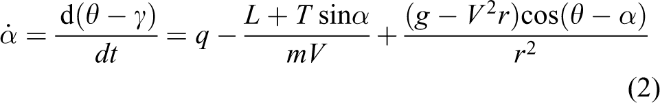
The model for a winged-cone configuration HFV’s flight dynamics developed by NASA Langley Research Center has presented in the literatures,^8,16,17 its parameters are provided in Table 1. And the vehicle’s longitudinal aerodynamic equations (the cruising Mach number is 15 and flight altitude is 110,000 ft) are

\dot{V} = \frac{T \cos α - D}{m} - \frac{g sin (θ - α)}{r^{2}}

\dot{α} = \frac{d (θ - γ)}{d t} = q - \frac{L + T sin α}{m V} + \frac{(g - V^{2} r) \cos (θ - α)}{r^{2}}

\dot{q} = \frac{M_{y y}}{I_{y y}}

\dot{θ} = q

\dot{h} = V sin (θ - α)

Table 1.

Aircraft and environment parameters.

Wing area, S	3603 (ft²)
Mean aerodynamic chord, $\bar{c}$	80 (ft)
Mass, m	9375 (slug)
Pitch axis moment of inertia, I_yy	7 × 10⁶ (lbf·ft)
Air density, ρ	0.24325 × 10⁻⁴ (slug/ft³)
Gravity constant, g	1.39 × 10¹⁶

where $V, α, q, θ, h$ , and γ are the flight speed, angle of attack, pitch angle rate, pitch angle, flight height, and flight path angle, respectively; r is the flight height from Earth’s center; T, D, L, and M_yy are the thrust, flight drag, lift, and pitch moment, respectively.

The related definitions of force and moment are given as

L = Q S C_{L}, D = Q S C_{D}, T = Q S C_{T}, M_{y y} = Q S C_{M} \bar{c}

where $Q = \frac{1}{2} ρ V^{2}$ is the dynamic press; $C_{L}, C_{D}, C_{T}$ , and C_M are the lift, drag, thrust, and pitch moment coefficients, respectively, this coefficients can be expressed as

C_{L} = 0.6203, C_{D} = 0.645 α^{2} + 0.0043378 α + 0.003772

C_{T} = {\begin{array}{l} 0.02576 δ_{T set}, δ_{T set} < 1 \\ 0.0224 + 0.00336 δ_{T set} otherwise \end{array}

C_{M} = C_{M} (α) + C_{M} (δ_{e}) + C_{M} (q) = - 0.035 α^{2} + 0.036617 α + 5.3261 \times 10^{- 6} + 0.0292 (δ_{e} - α) + (\frac{q \bar{c}}{2 V}) (- 6.79 α^{2} + 0.3015 α - 0.2289)

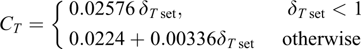
where δ_{T set} is the throttle setting and δ_e is elevator deflection. And the trimmed cruise condition of such HFV can be shown in Table 2 below.

Table 2.

The trimming condition.

Flight speed	15060 ft/s
Flight height	110000 ft
Angle of attack	0.0315 rad
Pitch angle rate	0 rad/s
Throttle setting	0.183
Elevator deflection	−0.0066 rad

HFV’s polynomial fitting model

Assumption 1

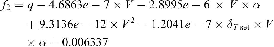
Since the value of θ − α is quite small during the cruise phase, we can simplify the sin and cosine function as $sin (θ - α) \approx (θ - α)$ and $\cos (θ - α) \approx 1$ in equations (1 to 5). And similarly, sinα ≈ α and cosα ≈ 1.

As the system ROA analysis is established by polynomial semi-positive definite programming, that means, the non-polynomial items in the traditional differential equation need to be fitted by polynomial.

With the multivariate nonlinear polynomial fitting method based on least squares,¹⁸ the non-polynomial items’ standard polynomial expression with specific parameters can be got by the “Minimize the SOS of deviations” principle. Using this method, the $\frac{1}{V}$ can be fitted as follow

\frac{1}{V} = 2.93 \times 10^{- 13} \times V^{2} - 1.32 \times 10^{- 8} \times V +1.99 \times 10^{- 4}

where $V \subseteq [\begin{matrix} 14, 960 ft / s & 15, 160 ft / s \end{matrix}]$ .

Substitute the parameters’ polynomial description and simplification into HFV’s longitudinal model in equations (1 to 5), then we can get the longitudinal five states polynomial normal system $\dot{x} = f (x, u)$ . As the longitudinal motion’s stability is mainly related to the kinetic equations, and the altitude can be computed directly by the flight speed, pitch angle and angle of attack in kinetic state in equation (7) below, so the altitude equation (5) can be omitted in our subsequent ROA analysis, and then the system states can be simplified as $x = [\begin{matrix} V & α & q & θ \end{matrix}]^{'}$ , the two inputs are $u = {[\begin{matrix} T & δ_{e} \end{matrix}]}^{'}$ . The HFV’s specific longitudinal polynomial system expressions can be got as

\dot{x} = f (x, u) = [\begin{matrix} f_{1} \\ f_{2} \\ f_{3} \\ f_{4} \end{matrix}]

where

f_{1} = 31.811 \times α - 31.811 \times θ - 3.0149 e - 6 \times ​ V^{2} \times α^{2} + 1.2041 e - 7 \times δ_{T set} \times V^{2} - 2.0272 e - 8 \times V^{2} \times α - 1.7631 e - 8 \times V^{2}

f_{2} = q - 4.6863 e - 7 \times V - 2.8995 e - 6 \times V \times α + 9.3136 e - 12 \times V^{2} - 1.2041 e - 7 \times δ_{T set} \times V \times α + 0.006337

f_{3} = 1.4624 e - 8 \times δ_{e} \times V^{2} - 4.5855 e - 6 \times V \times q - 1.7529 e - 8 \times V^{2} \times α^{2} + 3.7146 e - 9 \times V^{2} \times α + 2.6674 e - 12 \times V^{2} - 0.00013614 \times V \times α^{2} \times q + 6.0399 e - 6 \times V \times α \times q

f_{4} = q

The ROA estimation method based on V–s iteration

ROA estimation

For the nonlinear polynomial autonomous system

\dot{x} = f (x), x \in R^{n}, x (0) = x^{0}

where f(x) is the polynomial function with variation x, and f(0) = 0, the original state point is assumed to be local asymptotic stable equilibrium point.

The ROA of system, that is, the local asymptotic stability region of the system, is defined as

S = {x^{0} \in R^{n} | \lim_{t \to \infty} x (t, x^{0}) = 0}

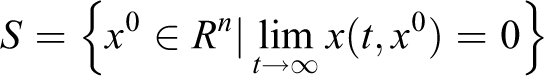
The estimation of ROA is to explore the system’s specific stable area. It’s difficult to compute the ROA exactly for nonlinear dynamical system, and there has been significant research devoted to the ROA’s invariant subsets estimation.

Lemma 1

If there exists a continuously differentiable function $V : R^{n} \to R$ such that¹⁹

V is positive definite

$Ω : = {x \in R^{n} | V (x) \leq 1}$ is bounded

${x \in R^{n} | V (x) \leq 1} \ {0} \subseteq {x \in R^{n} | \frac{\partial V}{\partial x} f (x) < 0}$

then for all

x (0) \in Ω

, the solution of Eq. (8) exists, satisfies

x (t) \in Ω

, and

\lim_{t \to \infty} x (t) = 0

. As such, Ω is invariant, and a subset of the ROA for Eq. (8), in which the continuously differentiable function V is called as local Lyapunov function.

In Figure 1, the ROA Ω defined by the solid line is an elliptical zone, and the $\dot{V} (x) = 0$ defined by the dot dash line is the boundary between positive and negative definite zone of V(x). The system ROA estimation is just finding the maximum ROA in the negative definite area which $\dot{V} (x) < 0$ .

Figure 1.

ROA estimation diagram. ROA: region of attraction.

In order to enlarge the ROA, we define a variable sized region²⁰

P_{β} = {x \in R^{n} | p (x) \leq β}

and then maximize β with the constraint $P_{β} \subseteq Ω$ . Here, the β is a positive value, and p(x) is a positive definite polynomial, which is chosen to reflect the different state parameters’ relative importance, it is called the shape factor. With the application of the lemma 1 above, the problem can be posed as the following optimization problem²⁰

\max_{V \in R^{n}} β,subject to

$V (x) > 0$ for all $x \in R^{n} / {0}$ and $V (0) = 0$

The set ${x \in R^{n} | V (x) \leq 1}$ is bounded

${x \in R^{n} | p (x) \leq β} \subseteq {x \in R^{n} | V (x) \leq 1}$

${x \in R^{n} | V (x) \leq 1} / {0} \subseteq {x \in R^{n} | \frac{\partial V}{\partial x} f < 0}$

With the S-procedure and SOS programming,¹⁹ the following sufficient conditions can be obtained based on the optimization conditions above

\underset{V \in R^{n}, V (0) = 0, s_{1}, s_{2} \in \sum_{n}}{\max β},subject to

$- [(β - p) s_{1} + (V - 1)] \in \sum_{n}$

$- [(1 - V) s_{2} + \frac{\partial V}{\partial x} f + l_{2}] \in \sum_{n}$

where s₁ and s₂ are SOS polynomials, and $l_{i} (x)$ is a positive definite polynomial of the form

l_{i} = \sum_{j = 1}^{n} ε_{i j} x_{j}^{2}

where $i = 1, 2$ and $ε_{i j}$ are positive numbers.

Advanced V–s iteration algorithm for ROA estimation

The constraint equations in the subsection above, contain some unknown variables, for example, β, V, and their products, such as the product of β and s₁, V and s₂. During the numerical solution process, these products will make that the SOS problem cannot be translated into a linear SDP, that is, bilinear problem.

To solve this bilinear problem, V–s iteration method will be introduced, the basic idea of V–s iteration is to divide the unknown variables into two groups. During this process, the two variables in product should be assigned to different groups, and one variables group is fixed to solve another group, and then exchanged for the next solution loop. With this process, the SOS problem can be transformed into linear SDP.

Moreover, the constraint condition in optimization problem above

{x \in R^{n} | p (x) \leq β} \subseteq {x \in R^{n} | V (x) \leq 1}

means that the variable sized region P_β is contained in the system’s ROA, or we can say that, for this constraint condition, the P_β with different “radius β” is used to enlarge or optimize the system’s ROA. So the shaper factor p(x) selection and ROA optimization has a very close relationship and the selection of p(x) will affect the ROA’s optimization.

To solve these problems, the advanced V–s iteration algorithm for ROA estimation is²⁰

1. Initialization: Compute the Jacobian matrix of f evaluated at x = 0

A = {\frac{\partial f (x)}{\partial x} |}_{x = 0}

Then solve the equation

A^{T} P + P A = - I

for a positive definite matrix P. Define

V (x) = x^{T} P x

p (x) = x^{T} P x

2. γ Step: Hold V fixed and solve the following SOS programming for $s_{2} (x)$

\underset{s_{2} \in \sum_{n}, γ \in R}{max γ^{*}},subject to

- [(γ - V) s_{2} + \frac{\partial V}{\partial x} f + l_{2}] \in \sum_{n}

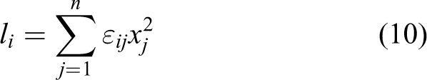
where l₂ is define in equation (10). The product problem of γ and s₂ can be solved by the conventional V–s iteration approach.^21,22

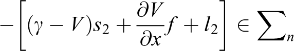
3. β Step: Hold V and p fixed and solve the following SOS programming for $s_{1} (x)$

\underset{s_{1} \in \sum_{n}, β \in R}{\max β^{*}},subject to

- [(β - p) s_{1} + (V - γ)] \in \sum_{n}

Similarly, such bilinear problem can be solved by the conventional V–s iteration approach.

4. V Step: Hold s₁, s₂, β*, γ*, and p fixed and compute V such that

- [\frac{\partial V}{\partial x} f + l_{2} + s_{2} (γ - V)] \in \sum_{n}

- [(V - γ) + s_{1} (β - p)] \in \sum_{n}

V - l_{1} \in \sum_{n}, V (0) = 0

where l₁ is defined in equation (10).

5. Scale V: Replace V with $V / γ^{*}$ . In this step, a new V is obtained which satisfies the constraints of the problem.

6. Update p: Replace the quadratic part of the new V as new p.

7. Repeat: Now with the new V and new p repeat the algorithm to reach to the maximum number of iterations.

To clearly demonstrate the optimization procedure of this advanced V–s iteration algorithm, the algorithm flow chart is shown as follow.

The maximum degree of V, s₁, and s₂ is restricted in this algorithm, that is, the maximum degree of these polynomials should satisfy

\begin{array}{l} \deg V \geq \deg l_{1} \\ \deg (p s_{1}) \geq \deg V \\ \deg s_{2} \geq \deg f - 1 \end{array}

where $\deg (*)$ defines the maximum degree of expression.

Closed-loop system analyses of HFV

In order to demonstrate the effectiveness of the proposed method, a simple and classical optimal quadratic controller design method is adopted for the aerodynamic equations (1 to 5) above. Firstly, the model is linearized at the trimming point

Δ \dot{x} = {\frac{\partial f (x, u)}{\partial x} |}_{x_{0}, u_{0}} Δ x + {\frac{\partial f (x, u)}{\partial u} |}_{x_{0}, u_{0}} Δ u = A Δ x + B Δ u

And then the controller can be got by the lqr command in Matlab^®

K = [\begin{matrix} 0.000005 & 0.002 & 0.0007 & 0.001 \\ - 0.0000023 & - 1.5599 & - 0.9699 & - 0.0002 \end{matrix}]

Substitute this controller into the polynomial nonlinear model equation. (7) to get the closed-loop system model below. With this closed-loop system expression, the HFV system’s ROA which is centered as trim point can be estimated.

\dot{x} = {f (x, u) |}_{u = u_{0} - K (x - x_{0})}

To complete the ROA estimation, we set whole programming iteration steps as N = 10. And for the γ and β steps in subsection “Advanced V–s iteration algorithm for ROA estimation”, we take the cycle overflow condition or tolerance $Δ γ = Δ β = 1.0 e^{- 5}$ , the initial value $γ_{0} = β_{0} = 0.0005$ , and define the $l_{i} (x)$ as

l_{1} = 1.0 e - 6 (V^{2} + α^{2} + q^{2} + θ^{2})

l_{2} = 1.0 e - 6 (V^{2} + α^{2} + q^{2} + θ^{2})

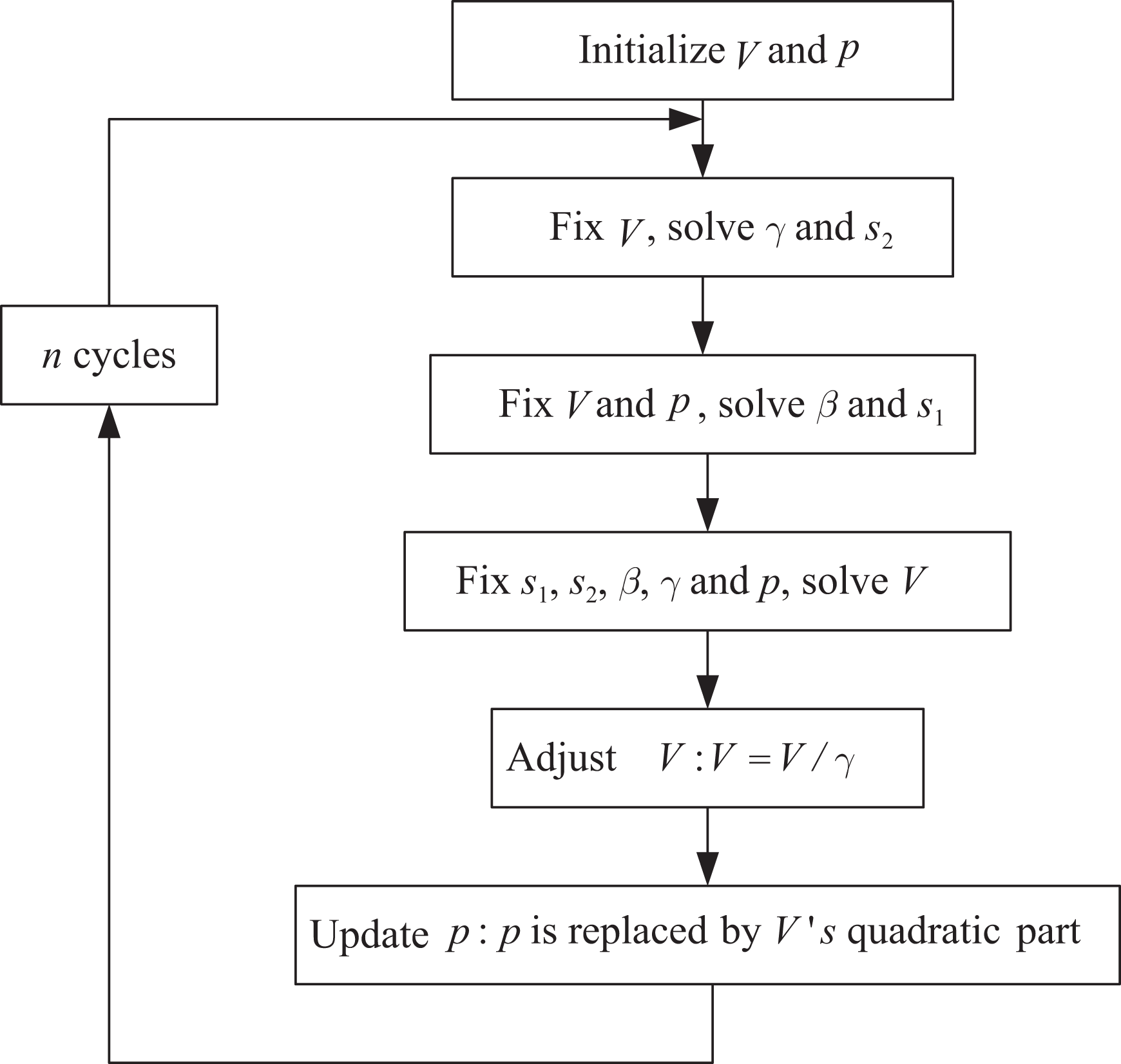
It is worth noting that the initial value $γ_{0} = β_{0}$ should be chose carefully to guarantee that the first programming step can be completed, and then the algorithm will normalize and optimize the corresponding objective parameter in Figure 2.

Figure 2.

Advanced V–s iteration algorithm flow chart.

With the advanced V–s iteration algorithm in subsection “Advanced V–s iteration algorithm for ROA estimation” and the initialization setting above, the ROA estimation results of normal aircraft can be got as Figure 3 below.

Figure 3.

ROA of closed-loop system 1. ROA: region of attraction.

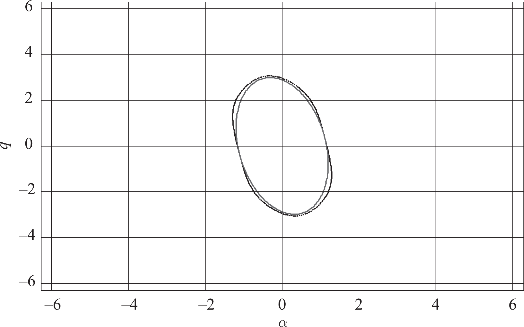
In Figure 3, the dotted line ellipse region $V (x) < γ$ is the ROA of system, and the solid line ellipse region $p (x) < β$ is the shape factor area. For HFV, if the initial flight condition is contained in such region, then its system states can converge to the initial condition when it confronts external or internal disturbance.

To show the benefit and effectiveness of nonlinear ROA estimation for flight control analysis, the system’s phase diagram is drawn in Figure 4 firstly and compared with the ROA region in Figure 5 below.

Figure 4.

Phase track of α and q.

Figure 5.

ROA of closed-loop system 2. ROA: region of attraction.

Figure 5 shows that, the nonlinear ROA estimation result contains most of the stable region of closed-loop system, and it captures the size of the stability region of the system. In engineering practice, it’s very difficult for the complex nonlinear system to complete the analytical solution or phase plane analysis, and the conventional linear analysis will miss some important characteristic of actual aircraft. The proposed method in this article can be used to verify the flight control system of HFV or analyze system’s stability.

Conclusions

The main contribution of this article is to present the polynomial modeling and ROA estimation approach for the HFV’s closed-loop system, which is helpful to complete the flight control verification. Such approach utilizes the polynomial model of NASA’ winged-cone configuration hypersonic vehicle and advanced V–s iteration algorithm to complete ROA estimation.

Case study results for the closed-loop HFV system were completed to show the validity of the proposed method. Further consideration should be focused on the integration problem between the controller design and ROA estimation for HFV.

Footnotes

Declaration of conflicting interests

The author(s) declared no potential conflicts of interest with respect to the research, authorship, and/or publication of this article.

Funding

The author(s) disclosed receipt of the following financial support for the research, authorship, and/or publication of this article: This work was partially supported by National Natural Science Foundation of China (61304098, 61622308), Natural Science Basic Research Plan in Shaanxi Province (2016KJXX-86) the Project Supported by Natural Science Basic Research Plan in Shaanxi Province of China (program No. 2015JQ6255), and Fundamental Research Funds of Shenzhen Science and Technology Project under grant JCYJ20160229172341417.

References

Sun

Yang

. Adaptive discrete-time controller design with neural network for hypersonic flight vehicle via back-stepping. Int J Control 2011; 84(9): 1543–1552.

Wilcox

MacKunis

Bhat

. Robust nonlinear control of a hypersonic aircraft in the presence of aerothermoelastic effects. In: IEEE American control conference, Hyatt Regency Riverfront, St. Louis, MO, USA, 10–12 June 2009, pp. 2533–2538.

Serrani

Zinnecker

Fiorentini

. Integrated adaptive guidance and control of constrained nonlinear air-breathing hypersonic vehicle models. In: IEEE American control conference, Hyatt Regency Riverfront, St. Louis, MO, USA, 10–12 June 2009, pp. 3172–3177.

Zhang

. Neural discrete back-stepping control of hypersonic flight vehicle with equivalent prediction model. Neurocomputing 2015; 154: 337–346.

Chen

Jiao

. Adaptive NN backstepping output-feedback control for stochastic nonlinear strict-feedback systems with time-varying delays. IEEE Trans Sys Man Cyber B Cyber 2010; 40: 939–950.

. Reinforcement learning output feedback NN control using deterministic learning technique. IEEE Trans Neural Network Learn Sys 2014; 25(3): 635–641.

Liu

. Nonlinear adaptive inversion control with neural network compensation for a longitudinal hypersonic vehicle model. In: IEEE international conference on intelligent computing and intelligent systems, Shanghai, China, 20–22 November 2009, pp. 264–268.

Mirmirani

Ioannou

. Adaptive sliding mode control design for a hypersonic flight vehicle. J Guid Control Dynam 2004; 27(5): 829–838.

Belcastro

. On the validation of safety critical aircraft systems, Part I: an overview of analytical and simulation methods. In: AIAA guidance, navigation, and control conference and exhibit, Austin, TX, USA, 11–14 August 2003, pp. 1–9.

10.

Chakraborty

Seiler

. Susceptibility of F/A-18 flight controllers to the falling leaf mode: linear analysis. J Guid Control Dynam 2011; 34(1): 57–72.

11.

Chakraborty

Seiler

. Susceptibility of F/A-18 flight controllers to the falling leaf mode: nonlinear analysis. J Guid Control Dynam 2011; 34(1): 73–85.

12.

Anderson

Papachristodoulou

. Robust nonlinear stability and performance analysis of an F/A-18 aircraft model using sum of squares programming. Int J Robu Nonlin Control 2013; 23(10): 1099–1114.

13.

Coutinho

Souza

. Local stability analysis and domain of attraction estimation for a class of uncertain nonlinear discrete-time systems. Int J Robu Nonlin Control 2014; 23(4): 1456–1471.

14.

Jackson

Kodoeorgiou

. Entrainment and migration controls of two-dimensional maps. Phys Lett D Nonlin Phenomena 1992; 54(3): 253–265.

15.

Parrilo

. Structured semi-definite programs and semi-algebraic geometry methods in robustness and optimization. Pasadena: California Institute of Technology, 2000.

16.

Marrison

Stengel

. Design of robust control systems for a hypersonic aircraft. J Guid Control Dynam 1998; 21(1): 58–63.

17.

Wang

Stengel

. Robust nonlinear control of a hypersonic aircraft. J Guid Control Dynam 2000; 23(4): 577–585.

18.

Han

Atkinson

. Theoretical numerical analysis—a functional analysis framework. Chap. 3, New York: Springer, 2009.

19.

Tan

Packard

. Stability region analysis using sum of squares programming. In: IEEE proceedings of the 2006 American control conference, Minneapolis, MN, USA, 14–16 June 2006, pp. 2297–2302.

20.

Jarvis-Wloszek

. Lyapunov based analysis and controller synthesis for polynomial systems using sum-of-squares optimization. Berkeley: University of California, 2003.

21.

Chakraborty

Seiler

Balas

. Nonlinear region of attraction analysis for flight control verification and validation. Control Eng Pract 2011; 19(4): 335–345.

22.

Khodadadi

Samadi

Khaloozadeh

. Estimation of region of attraction for polynomial nonlinear systems: a numerical method. ISA Trans 2014; 53(1): 25–32.

Nonlinear region of attraction analysis for hypersonic flight vehicles’ flight control verification

Abstract

Keywords

Introduction

Hypersonic vehicle models

Longitudinal model description

HFV’s polynomial fitting model

Assumption 1

The ROA estimation method based on V–s iteration

ROA estimation

Lemma 1

Advanced V–s iteration algorithm for ROA estimation

Closed-loop system analyses of HFV

Conclusions

Footnotes

Declaration of conflicting interests

Funding

References