Sage Journals: Discover world-class research

Abstract

This article proposes a composite path following controller that allows the small fixed-wing unmanned aerial vehicle to follow a predefined path. Assuming that the vehicle is equipped with an autopilot for altitude and airspeed maintained well, the controller design adopts the hierarchical control structure. With the inner-loop controller design based on the notion of active disturbance rejection control which will respond to the desired roll angle command, the core part of the outer-loop controller is designed based on Lyapunov stability theorem to generate the desired course rate for the straight-line paths. The bank to turn maneuver is used to transform the desired course rate to the desired roll angle command. Both the hardware-in-the-loop simulation in the X-Plane simulator and actual experimental flight tests have been successfully achieved, which verified the effectiveness of the proposed method.

Keywords

Path following small unmanned aerial vehicle Lyapunov stability ADRC

Introduction

Unmanned aerial vehicles (UAVs) have been wildly developed in diverse military and civilian application domains in the last decade. The small fixed-wing UAVs have been applied in the polar environment observation,^1,2 monitoring moving objects,³ testing the new control strategies,^4,5 and many other domains. In terms of advanced control technologies, path planning,^2,3,6 cooperative control,^6,7 and obstacle avoidance⁸ have been designed, tested, and applied in fixed-wing UAVs in recent years. It can be seem that it is critical for the vehicles to track or follow the predefined path or trajectory accurately so that they can realize these technologies.

During recent years, the approaches to realize the path following or trajectory tracking control of a small UAV appear on the linear and nonlinear control methods. The linear techniques include the proportion–integration–differentiation (PID) and linear quadratic regulator (LQR), while the nonlinear methods mostly appear on the backstepping technique, the fuzzy logic-based control, the sliding mode control, and the model predictive control (MPC).

In the study of Kohno and Uchiyama,⁹ the outer-loop design for translational motion is based on the proportion-differentiation (PD) controller together with the disturbance accommodating control method to estimate the aerodynamic force. Comparing to the traditional PID technique, Luo et al. applied the directional fractional order (PI)α method to the lateral control of a small fixed-wing UAVs based on the decoupled single input single output (SISO) mathematical model.¹⁰ However, the PID controller has little robustness to the disturbance, and it is mostly used in the lateral/longitudinal maneuvers by reducing the lateral deviation from a desired fight path. The genetic algorithm has also been used to optimize the control parameters of the trajectory tracking control law which will improve the tracking performance.¹¹ However, it needs more calculation, which makes it limited to be applied on the low-cost autopilot. In the study of Ratnoo et al.,¹² the LQR with an adaptive running cost was applied to generate the lateral acceleration command to guide the vehicle toward the path. Lee et al. used the LQR technique to reach the path following by finding the optimal state feedback law where its state is the combination of the lateral attitudes, the crosstrack, and heading errors.¹³ However, the heading and crosstrack errors should be saturated to make the system stable due to the limitation of the linear region.

In the aspect of nonlinear control of path following, the backstepping technique has been applied to the path following of the fixed-wing aircraft. In the study of Brezoescu et al.,¹⁴ the adaptive backstepping was applied to reach the trajectory following considering the influence of the crosswind, and the method was verified in simulation. Jung and Tsiotras used the adaptive backstepping to the path following through roll angle control.¹⁵ Sartori et al.¹⁶ combined backstepping with the PID controller to realize the control of the fixed-wing UAV, where the outer loop for guidance adopted the PID method. The backstepping was used for the control of attitude. While applying the backstepping technique, it will introduce additional control parameters or it needs good knowledge of the nonlinear system.

The fuzzy logic is another technique applied to the guidance of the UAV. Cancemi et al. applied the fuzzy logic to generate the heading reference which will guide the UAV toward the predefined waypoint trajectory.¹⁷ The fuzzy-based method was implemented in the hardware-in-the-loop simulation. In the study of Gomez and Mo,¹⁸ the fuzzy logic was applied to control the UAV with the decentralized model to drive the tracking error to zero. The fuzzy logic method can reach better tracking performance than the traditional PID controller, but it needs more memory to store the rules and values for the fuzzy logic which will result in additional calculation.

In the studies of Lei et al.,² Beard et al.,¹⁹ Nelson et al.,²⁰ and Liang et al.,²¹ the tangent vector filed concept together with the sliding mode control technique was applied to design the course to achieve the curved path following with given constant wind disturbances. The slide mode controller is interesting and suitable for the actual flight, but it is known to have the chattering problem due to the controller’s inherent discontinuity.

The MPC is an alternative method for path following since it can combine multiple objectives and constraints, which minimize the objective function. Yang et al. presented an adaptive nonlinear MPC controller for the path following of a fixed-wing UAV with the variable control horizon depending upon the path curvature profile, and the adaptive scheme was verified by simulation comparing with a conventional fixed-horizon MPC.⁸ Prodan et al.²² applied the MPC for trajectory tracking of UAV, where the core MPC algorithm was run in MATLAB (Product of the MathWorks, Inc) off-board to generate the guidance law which was sent to the onboard avionic through communication link. The above scenarios indicate that the MPC method is robust for path following, but it needs much more numerical calculation which makes it difficult to be applied in the low-cost onboard flight control system.

Motivated by the above discussion, this article aims to realize the path following of a small fixed-wing UAV in the two-dimensional (2-D) plane with low-cost avionics which can provide altitude- and airspeed-hold functions. In this article, we adopted the hierarchical control architecture for the path following control system design. In our preview works,²³ a Lyapunov stable–based nonlinear control law has been designed to generate the course rate command as the core part of the outer-loop controller. The nonlinear control law has been demonstrated by the Lyapunov stability arguments that it will guide the vehicle to fly along the desired line path with the right direction. The above has been demonstrated via the Aerosonde UAV model in the MATLAB simulation.²³ In this article, we have transformed the commanded course rate into the reference commanded bank angle for the inner controller by using the bank to turn maneuver.

For the inner controller design, in contrast to previous methods, the active disturbance rejection control (ADRC)^24
–26 which has been applied in various areas will be applied. Since it is difficult to model the dynamics of a small fixed-wing UAV with accurate parameters, even the disturbance including the turbulent flow and the actuator installation errors, the ADRC contains an extended state observer (ESO)²⁴ which can directly estimate the system dynamics and the disturbance, which are extended as a new system state. Together with other two parts of ADRC, a tracking differentiator (TD) and a nonlinear control, the ADRC is used here as the inner loop to realize tracking the reference bank angle.

The contribution of this article is that the proposed path following controller was firstly successfully applied on the actual fixed-wing UAV flight. The organization of this article is as follows. In the next section, a brief description of the UAV is given, and the hierarchical control architecture for the path following control system design is proposed. In “Outer-loop controller” section, the core part of the outer-loop controller is designed based on the Lyapunov stable arguments to generate the desired course rate for straight-line paths, and the desired course rate is transformed into the reference bank angle using the bank to turn maneuver. In “ADRC-based inner-loop control law” section, the ADRC method is applied to realize the bank angle tracking. The hardware-in-the-loop simulations and flight tests of the UAV are presented in “Simulations and experiments” section. Finally, some concluding remarks are summarized in “Conclusion” section.

System description

The Snow Goose UAV (Figure 1(a)) is approximately 2.2 m long with an approximately 3.2 m wingspan. The aircraft has a takeoff weight of approximately 25 kg, including an approximately 3 kg electronic payload. A single-cylinder two-cycle piston value type gasoline engine is installed to provide the thrust. The fuel capacity is approximately 3 L of jet fuel for maximum mission duration of approximately 4 h at cruise flight.

Figure 1.

The UAV platform for the experiments: (a) the Snow Goose UAV and (b) onboard avionics. UAV: unmanned aerial vehicle.

The avionics (Figure 1(b)) used to implement the automatic control contains a navigation system, an embedded flight control system, and a data communication system. The navigation system consists of three axis magnetometers (a single-axis HMC1041, A Product of Honeywell International Inc., USA and a two-axis HMC 1052, A Product of Honeywell International Inc., USA), two pressure sensors (MS5540CM, A Product of TE Connectivity Ltd., USA. and MPXV5004GP, A Product of Freescale Semiconductor, Inc., USA.), a Differential Global Positioning System (DGPS) receiver, and an Inertial Measurement Unit (IMU) unit (ADSL16355, A Product of Analog Devices, Inc., USA.). The extended Kalman filter algorithm is used to fuse the values of above sensors. A Field-Programmable Gate Array (FPGA)-based input/output (I/O) board was integrated in the flight control system to drive the onboard digital servos and to read pilot commands through a standard Futaba transmitter. The avionics systems have an accuracy of 0.2 m root mean square (RMS) for the position, 0.03 m/s RMS for the linear velocity, and 0.017 rad RMS for the attitude. During the experiment, all vehicle state variables were sampled at 50 Hz and recorded in a 4 GB flash memory on the flight control system.²⁷

To realize the accurate path following of UAV, even in the presence of wind disturbance, we assume that the altitude and the airspeed are maintained well. Figure 2 shows the flowchart of the proposed robust path following controller. The controller is hierarchically divided into two layers: (1) The core task of the inner-loop control layer is to realize the bank angle tracking considering the disturbance including the turbulent flow and the actuator installation errors. (2)The outer-loop control layer is to guarantee the path following performance for the predefined flight tasks. In this layer, the core part of the controller gets the current position and heading information from the navigation system, and then generates the desired course rate command u_cmd through the error information between the current position and the predefined path. Finally, the outer-loop controller generates the desired bank angle φ_c by using the bank to turn maneuver. The update cycle of the controller is 20 ms.

Figure 2.

The flight control structure of the UAV. UAV: unmanned aerial vehicle.

Outer-loop controller

Problem description

The outer-loop controller design focuses on the navigation of the UAV. The assumptions that the small fixed-wing UAV equipped with low-level flight controller can provide altitude- and airspeed-hold functions are used for the path following. The kinematics of the UAV in the Earth-fixed horizontal frame considering the wind velocity W = (W_x,W_y) can be modeled as follows

{\begin{matrix} \dot{x} = V_{a} cos (ψ) + W_{x} \\ \dot{y} = V_{a} sin (ψ) + W_{y} \end{matrix}

where (x,y) is the inertial position of the UAV, V_a is the airspeed, and ψ is the heading. By introducing the ground speed V_g and the course χ shown in Figure 3,²³ equation (1) can be expressed as

{\begin{matrix} \dot{x} = V_{g} cos (χ) \\ \dot{y} = V_{g} sin (χ) \end{matrix}

Figure 3.

Position of the UAV with respect to the desired line and the relationship among the ground speed V_g, airspeed V_a, and the wind speed W. UAV: unmanned aerial vehicle.

Following the study of Nelson et al.,²⁰ by introducing the course rate control $\dot{χ} = u_{cmd}$ , the system (2) becomes

{\begin{matrix} \dot{x} = V_{g} cos (χ) \\ \dot{y} = V_{g} sin (χ) \\ \dot{χ} = u_{cmd} \end{matrix}

Therefore, the motions of the UAV can be expressed in terms of the ground speed and the course angle. In the following, the command design is based on the model (3). Since the ground speed contains the information of wind velocity, the wind disturbance rejection will be naturally considered. Just as all of the 2-D curve can be approximated by a series of segments, we focus on the UAVs’ line following below.²³

Straight-line path following

In this subsection, the brief description of the straight-line path following control law is based on our preview works.²³ In Figure 3, the desired straight-line path of the UAV can be expressed as

a x + b y + c = 0

where the parameters of the line path function (4) subject to |a| + |b| > 0.

Let D(x,y) denotes the deviation of the UAV position from the desired line, then

D (x, y) = \frac{a x + b y + c}{\sqrt{a^{2} + b^{2}}}

For the system (3), the following control law²³ is introduced that will guarantee its stability

u_{cmd} = - K_{1} V_{g} f_{sat} (D (x, y)) - K_{2} V_{g} \frac{d D (x, y)}{d t}

where K₁ and K₂ are positive constants, and the saturation function f_sat(x) is defined as

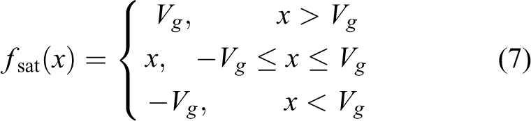
f_{sat} (x) = {\begin{matrix} V_{g}, x > V_{g} \\ x, - V_{g} \leq x \leq V_{g} \\ - V_{g}, x < V_{g} \end{matrix}

Here, the function f_sat(x) is used to limit the distance D(x,y) so that the control law (6) will always be within a given range, even the initial value of D(x,y) is very large.

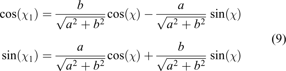
In order to analyze the stability of the line tracking control law (6), two new variables d₁ and χ₁ are introduced as follows

\begin{matrix} d_{1} = D (x, y) \\ χ_{1} = {\begin{matrix} χ - {tan}^{- 1} (- a / b), if b \neq 0 \\ χ - π / 2, if b = 0, and a < 0 \\ χ + π / 2, if b = 0, and a > 0 \end{matrix} \end{matrix}

So we have

\begin{matrix} \cos (χ_{1}) = \frac{b}{\sqrt{a^{2} + b^{2}}} \cos (χ) - \frac{a}{\sqrt{a^{2} + b^{2}}} sin (χ) \\ sin (χ_{1}) = \frac{a}{\sqrt{a^{2} + b^{2}}} \cos (χ) + \frac{b}{\sqrt{a^{2} + b^{2}}} sin (χ) \end{matrix}

Equation (8) shows that if the UAV is flying along the desired line with the right direction, then d₁ = 0 and χ₁ = 0. By taking the derivatives of these two new variables d₁ and χ₁, we have

\begin{matrix} {\dot{d}}_{1} = \frac{d D (x, y)}{d t} = \frac{a \dot{x} + b \dot{y}}{\sqrt{a^{2} + b^{2}}} \\ = \frac{a V_{g} \cos (χ) + b V_{g} sin (χ)}{\sqrt{a^{2} + b^{2}}} \\ = V_{g} sin (χ_{1}) \\ {\dot{χ}}_{1} = - K_{1} V_{g} f_{sat} (D (x, y)) - K_{2} V_{g} \frac{d D (x, y)}{d t} \\ = - K_{1} V_{g} f_{sat} (d_{1}) - K_{2} V_{g}^{2} sin (χ_{1}) \end{matrix}

In the study of Chen et al.,²³ it has been demonstrated that if K₁ is a positive constant, V_g ≥ V_gp and $K_{2} = K_{2} (t) \geq K_{2 p}$ , where V_gp and K_2p are positive constants, then the uniformly asymptotically stable equilibrium points of the system (10) equal the set ${(d_{1}, χ_{1}) | d_{1} = 0, χ_{1} = 2 k π, k \in Z}$ . The brief demonstration is shown below.

Proof

Rewrite the system (10) as $\dot{x} = g (x, t)$ with $x = {[d_{1}, χ_{1}]}^{T}$ and $g (x, t)$ defined as

g (x, t) = [\begin{matrix} V_{g} sin (χ_{1}) \\ - K_{1} V_{g} f_{sat} (d_{1}) - K_{2} V_{g}^{2} sin (χ_{1}) \end{matrix}]

Let $\dot{x} = g (x, t) = 0$ . Since V_g ≥ V_gp > 0, then the solutions to $g (x, t) = 0$ are the set ${(d_{1}, χ_{1}) | d_{1} = 0, χ_{1} = k π, k \in Z}$ . Firstly, the stable equilibrium points are the set ${(d_{1}, χ_{1}) | d_{1} = 0, χ_{1} = 2 k π, k \in Z}$ . Without loss of generality, we consider the equilibrium point (0,0). Define the domain $D = {(d_{1}, χ_{1}) | d_{1} \in R, - π < χ_{1} < π}$ .

The Lyapunov candidate function is chosen as $V (t, x) = K_{1} \int_{0}^{d_{1}} f_{sat} (y) d y + \int_{0}^{χ_{1}} sin (y) d y$ . Since $\int_{0}^{d_{1}} f_{sat} (y) d y > 0$ and $\int_{0}^{χ_{1}} sin (y) d y = 1 - \cos (χ_{1}) > 0$ for all $x \in D - {0}$ , if K₁ > 0, then V(t,x) > 0 on D − {0}.

Furthermore, $V (t, x) = K_{1} \int_{0}^{d_{1}} f_{sat} (y) d y + 1 - \cos (χ_{1}) \leq (K_{1} / 2) d_{1}^{2} + 1 - \cos (χ_{1}) \leq (K_{1} / 2) d_{1}^{2} + 1 - \cos (χ_{1}) = W_{1} (d_{1}, χ_{1})$ . $V (t, x) \geq 1 - \cos (χ_{1}) = 2 {sin}^{2} (χ_{1} / 2) = W_{2} (d_{1}, χ_{1})$ .

Additionally, it has the fact that $\dot{V} (t, x) = (\partial V / \partial t) + (\partial V / \partial x) g (x, t) = 2 (K_{1} {\dot{d}}_{1} f_{sat} (d_{1}) + {\dot{χ}}_{1} sin (χ_{1})) = - 2 K_{2} V_{g}^{2} {sin}^{2} (χ_{1}) \leq - 2 K_{2} V_{g p}^{2} {sin}^{2} (χ_{1}) = - W_{3} (d_{1}, χ_{1})$ .

It can be derived that W₁(d₁,χ₁), W₂(_d₁,χ₁), and W₃(d₁,χ₁) are continuous positive definite functions on the domain D. Then, the equilibrium point (0, 0) is uniformly asymptotically stable. Similarly, the equilibrium points in the set ${(d_{1}, χ_{1}) | d_{1} = 0, χ_{1} = 2 k π, k \in Z}$ are all uniformly asymptotically stable. The detailed demonstration that the points in the set ${(d_{1}, χ_{1}) | d_{1} = 0, χ_{1} = (2 k + 1) π, k \in Z}$ are all unstable can be seen in the study of Chen et al.²³

Bank to turn maneuver

For 2-D path following, the bank to turn maneuver is used to realize the UAV’s level turn. In this case, the UAV maintains a constant altitude with no sideslip. Figure 4 shows the forces acting on the UAV under the mode of bank to turn maneuver. By applying Newton’s first law of motion, the kinematic and dynamic relationships can be found. The total lift can be broken into two components, where the vertical component of lift opposes the aircraft’s weight F_G. Since the UAV maintains at a constant altitude, the amplitude of the vertical component of lift equals the aircraft’s weight. On the other hand, the horizontal component of lift is used to turn the UAV, and it equals the centrifugal force F_c.

Figure 4.

UAV in a level turn. UAV: unmanned aerial vehicle.

So it gets the fact that

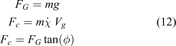
\begin{matrix} F_{G} = m g \\ F_{c} = m \dot{χ} V_{g} \\ F_{c} = F_{G} tan (φ) \end{matrix}

where m is the mass of the UAV, g is the acceleration of gravity, and φ is the bank (roll) angle. For a given course rate command $\dot{χ} = u_{cmd}$ , it can be consequently translated into a bank angle command φ_c as

φ_{c} = \arctan (\frac{V_{g} u_{cmd}}{g})

Since the inertial speed can be measured by the present avionics system, with the description of the straight line following course rate command, the relative bank angle command can be naturally achieved.

ADRC-based inner-loop control law

Modeling of the bank to turn dynamics

In this article, for designing an inner-loop control law to track the roll angle command, it is necessary to know the basic relationship between the control inputs and the roll angle output. The model with reduced set of first-order differential equations can be described as²⁸

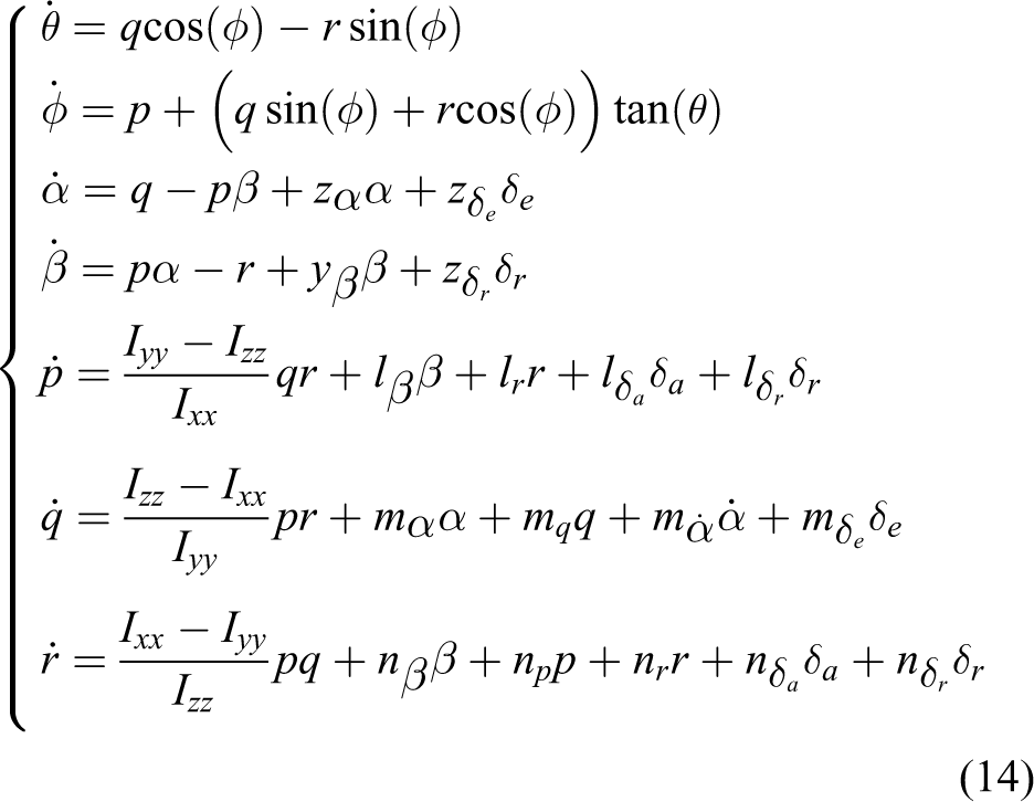
{\begin{cases} \dot{θ} = q \cos (φ) - r sin (φ) \\ \dot{φ} = p + (q sin (φ) + r \cos (φ)) tan (θ) \\ \dot{α} = q - p β + z_{α} α + z_{δ_{e}} δ_{e} \\ \dot{β} = p α - r + y_{β} β + z_{δ_{r}} δ_{r} \\ \dot{p} = \frac{I_{y y} - I_{z z}}{I_{x x}} q r + l_{β} β + l_{r} r + l_{δ_{a}} δ_{a} + l_{δ_{r}} δ_{r} \\ \dot{q} = \frac{I_{z z} - I_{x x}}{I_{y y}} p r + m_{α} α + m_{q} q + m_{\dot{α}} \dot{α} + m_{δ_{e}} δ_{e} \\ \dot{r} = \frac{I_{x x} - I_{y y}}{I_{z z}} p q + n_{β} β + n_{p} p + n_{r} r + n_{δ_{a}} δ_{a} + n_{δ_{r}} δ_{r} \end{cases}

where θ and φ represent the pitch and bank angles, respectively. α and β denote the angles of attack and sideslip, respectively. p, q, and r are the rigid body angular rates, respectively. δ_e, δ_a, and δ_r are elevator, aileron, and rudder deflections, respectively. I_xx, I_yy, and I_zz are the moments of inertia with respect to the rigid body coordinates, respectively. z_α, $z_{δ_{e}}$ , y_β, $z_{δ_{r}}$ , l_β, l_r, $l_{δ_{a}}$ , $l_{δ_{r}}$ , m_α, m_q, $m_{\dot{α}}$ , $m_{δ_{e}}$ , n_β, n_p, n_r, $n_{δ_{a}}$ , and $n_{δ_{r}}$ are coefficients.

Taking the derivatives of the both sides of the second part of equation (14) with respect to time, one can derive the relationship between the aileron deflection δ_a and the roll angle φ as

\ddot{φ} = f (φ, \dot{φ}, ϖ (t), t) + k_{3} δ_{a}

where k₃ is a constant, f is the function with respect to θ, φ, α, β, p, q, r, δ_e, and δ_r. By combining like terms, we can get the function f with the expression (15). φ, α, β, p, q, r, and δ_e are all contained in the coefficients of the terms with respect to $\dot{φ}$ and $\ddot{φ}$ . The terms with respect to δ_r are expressed as ϖ(t), which is treated as a disturbance. Actually, the turbulent flow and the actuator installation errors which will influence the dynamic of bank to turn maneuver can also be added to ϖ(t).

ADRC for bank angle tracking

Equation (15) describes the relationship between the control input δ_a and the bank angle φ. The goal of the following aims at tuning δ_a so that the UAV will track the desired bank angle φ_c. Since the function $f (φ, \dot{φ}, ϖ (t), t)$ contains so much information, even some unknown disturbance, it is difficult to find the analytic solutions to equation (15). However, for the above second-order system, by treating the function $f (φ, \dot{φ}, ϖ (t), t)$ as an unknown term, the ESO of the ADRC²⁴ can estimate it.

Let x₁ = φ, $x_{2} = \dot{φ}$ , and $x_{3} = f (φ, \dot{φ}, ϖ (t), t)$ , and then the system (15) is initially increased as

\begin{matrix} {\dot{x}}_{1} = x_{2} \\ {\dot{x}}_{2} = x_{3} + k_{3} δ_{a} \\ {\dot{x}}_{3} = \dot{f} \\ y = x_{1} \end{matrix}

where y is the output measured and to be controlled. $f (φ, \dot{φ}, ϖ (t), t)$ is treated as an increased state. As mentioned above, the assumption that f and $\dot{f}$ are unknown is adopted. By considering $f (φ, \dot{φ}, ϖ (t), t)$ as a state, Han proposed a nonlinear observer for equation (16) including estimating the increased state x₃ as^24,26

\begin{matrix} e = z_{1} - y \\ f e = f a l (e, 0.5, δ), f e_{1} = f a l (e, 0.25, δ) \\ {\dot{z}}_{1} = z_{2} - β_{01} e \\ {\dot{z}}_{2} = z_{3} + k_{3} u - β_{02} f e \\ {\dot{z}}_{3} = - β_{03} f e_{1} \end{matrix}

where e is the observer error, and the function fal(e,α,δ) is defined as²⁴

f a l (e, α, δ) = {\begin{matrix} \frac{e}{δ^{1 - α}}, | e | < δ \\ {| e |}^{α} sign (e), | e | > δ \end{matrix}

in which (·) denotes a standard sign function. δ > 0 is the control parameter which will influence the noise suppression, and it can be chosen from the range of [0.0001, 1].^25,26 β₀₁, β₀₂, and β₀₃ are positive observer gains.

Figure 5 shows the schematic diagram of the ADRC for tracking the bank angle command. Besides the nonlinear observer, the ADRC contains two other parts, that is, a TD in the feedforward path and a nonlinear proportional derivative (NPD) control synthesizer in the feedback path. The TD is used to solve the difficulties posed by low-order reference trajectories. In practice, the discrete time system (19) can be used as a high-performance TD to provide two signals v₁(t) and v₂(t), such that v₁(t) → φ_c(t) and $v_{2} (t) \to {\dot{φ}}_{c} (t)$ , respectively^24,25

\begin{matrix} v_{1} (k + 1) = v_{1} (k) + h v_{2} (k) \\ v_{2} (k + 1) = v_{2} (k) + h f h a n (v_{1} (k) - φ_{c} (k), v_{2} (k), r_{0}, h_{0}) \end{matrix}

Figure 5.

The ADRC for tracking the bank angle command φ_c. ADRC: active disturbance rejection control.

where h is the sampling period, k denotes the k_th sampling instant, and r₀ and h₀ are control parameters which determine the tracking speed and the effect of noise suppression, respectively. The details of function fhan can be found in the study of Han.²⁴

Therefore, with the output singles v₁ and v₂ generated from TD and the estimation of the state from ESO, the differential signals e₁ and e₂ can be obtained. Then, with these two signals as inputs, the NPD control synthesizer is defined as^25,26

\begin{matrix} e_{1} = v_{1} - z_{1} \\ e_{2} = v_{2} - z_{2} \\ u_{0} = k_{1} f a l (e_{1}, α_{1}, δ) + k_{2} f a l (e_{2}, α_{2}, δ) \end{matrix}

where k₁, k₂, α₁, and α₂ are control parameters and 0 < α₁ < 1 < α₂. With appropriate parameters and the estimation of $f (φ, \dot{φ}, ϖ (t), t)$ from the ESO, the total control law of the ADRC can be derived as

δ_{a} = u_{0} - \frac{z_{3}}{k_{3}}

Simulations and experiments

In this section, both the simulation and actual implementation results based on the proposed control method are presented. Table 1 lists the control parameters of the nonlinear control law and the ADRC.

Table 1.

Control parameters.

Parameter	Value	Parameter	Value	Parameter	Value
K ₁	0.0004	β ₀₃	100	k ₂	0.3
K ₂	0.018	δ	0.05	α ₁	0.5
h	0.05	r ₀	5000	α ₂	1.25
β ₀₁	20	h ₀	0.05	k ₃	160
β ₀₂	55	k ₁	2

Hardware-in-the-loop simulation

The simulation is taken in the X-Plane platform²⁹ with the hardware in the loop. Figure 6 shows the configuration of the simulation system, which consists of the flight control module, ground station, and a special computer used for running the X-Plane software Product of Laminar Research. The flight control module is connected to the ground station via a serial cable using the standard RS-232 serial protocol. The ground station sends the control parameters and predefined path to the flight control module and monitors its running. The X-Plane simulator is connected to the flight control module via a serial cable, and their data communication protocol is User Datagram Protocol. The X-Plane simulator receives the control commands from the flight control module and sends the responding states back to it via FlightSim framework middleware.

Figure 6.

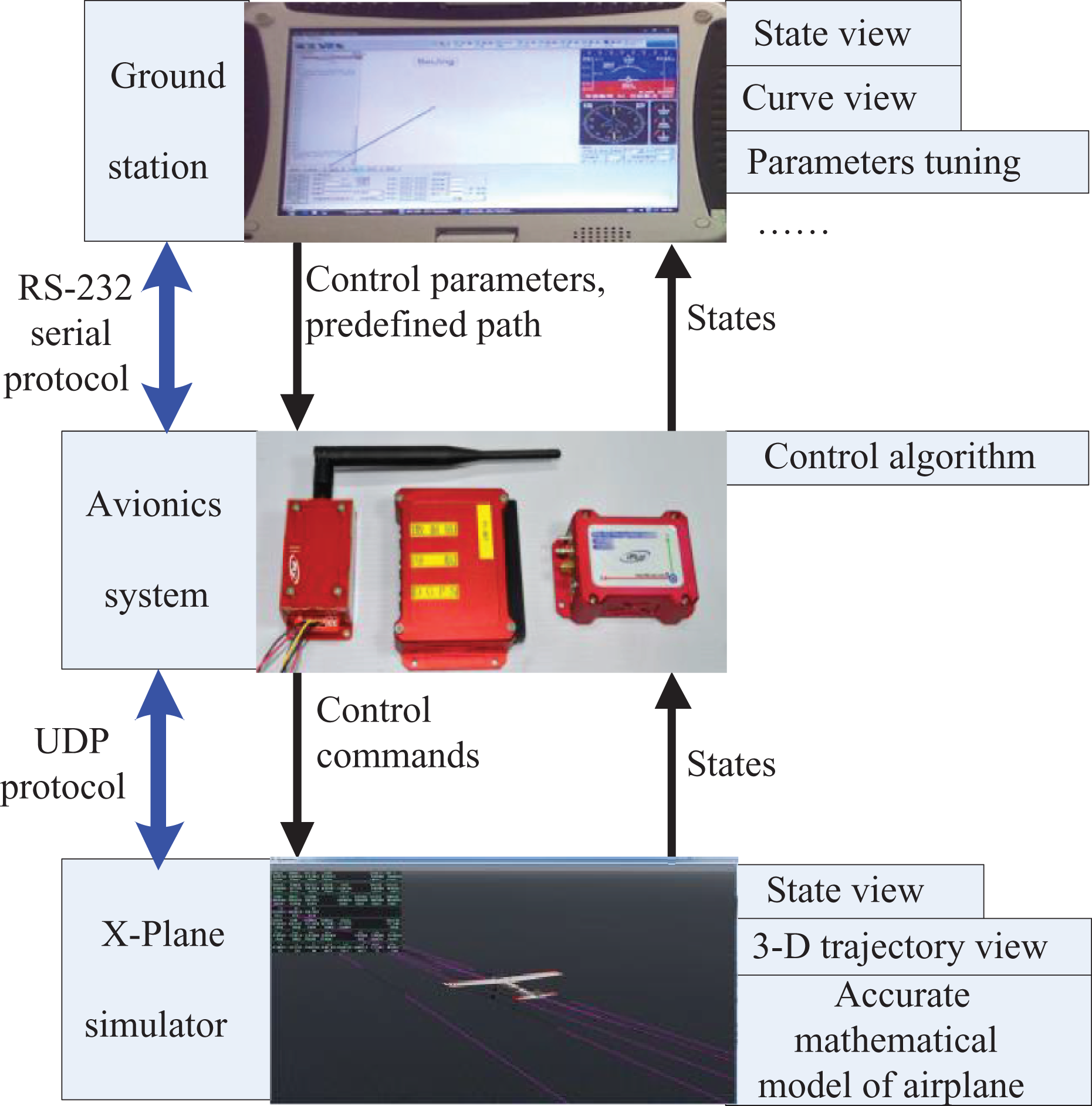
The configuration of the hardware-in-the-loop simulation.

The predefined path was a pentagon as shown in Figure 7. For simulation, the initial horizontal ground speed of the UAV was set as 20 m/s. In order to test the performance of the proposed controller, additionally, the external wind disturbance was added while simulating.

Figure 7.

Predefined path following with the proposed method in the X-Plane simulator.

The sharp changes of D(x,y) with about 120 m in Figure 8(a) are caused by the predefined behavior that the UAV will switch course if the distance between the position of the UAV and the next waypoint is smaller than 120 m, which can also be seen in Figure 7. The inertial velocity V_g shown in Figure 8(b) indicates the influence of the external disturbance. Especially when the UAV was following the path from point E to point A, the inertial velocity V_g reached 28 m/s. However, the steady-state error D(x,y) when the UAV followed the segments CD and EA was within 3 m and 2 m, respectively, as shown in Figure 8(a).

Figure 8.

The hardware-in-the-loop simulation results while following the predefined path in the X-Plane simulator: (a) the offset distance D(x,y), (b) the inertial velocity V_g, and (c) the comparison of the bank angle command φ_c and the simulated bank angle φ.

Figure 8(c) shows that the inner-loop controller ADRC can tracked the bank angle command φ_c well while following the predefined path. The above discussion demonstrated the effectiveness of the proposed path following controller even in the presence of the wind disturbance.

Actual flight test result

Figure 9(a) shows an actual outdoor flight test of the Snow Goose UAV with the proposed path following controller. The flight area was performed in a 600 × 1500 m region with constant height of 200 m. The normal flight speed was set as 20 m/s, and the inertial velocity V_g shown in Figure 9(b) indicates the influence of the external disturbance. In the actual flight, the UAV switched course in advance with 60 m. The zoom area in Figure 9(c) shows that the largest offset distance was about 10.3 m when the UAV was switching from segment DE → EA at time 117 s. Compared with following segments AB–BC, there is some larger amplitude while following the segments CD–DE–EA. Since the segments CD and DE are both shorter than AB and BC, the vehicle will switch course faster before it has realized the precise path following. It indicates that the predefined path should be planned well to make the vehicle get better path following performance.

Figure 9.

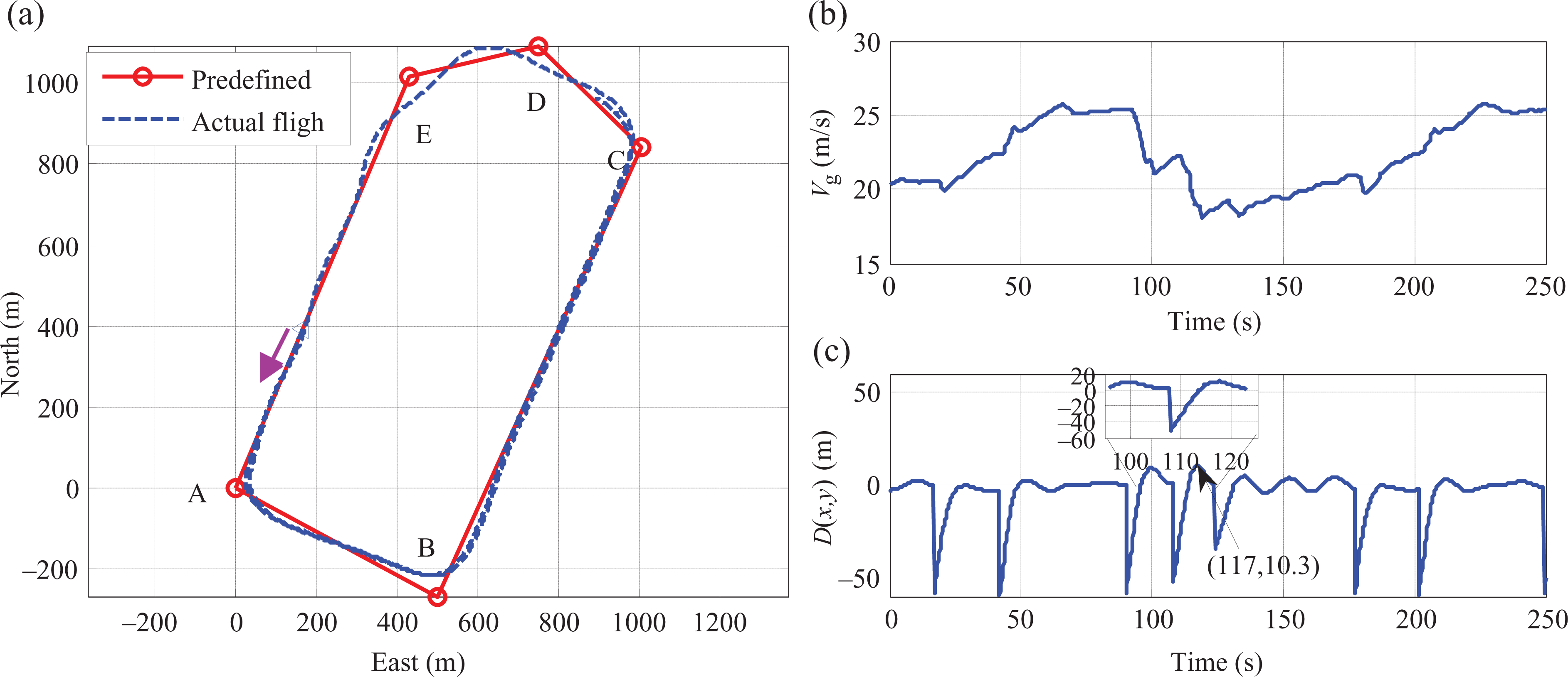
Actual path following with the proposed method: (a) predefined and actual flight path; (b) the inertial velocity V_g; and (c) the offset distance D(x,y).

All of the above has verified that the UAV can realize good path following motion with the proposed method.

Conclusion

With the combination of Lyapunov stability theory and ADRC technique, a line-style path following controller has been designed and implemented for a small fixed-wing UAV using the bank to turn maneuver. For the inner loop, the ADRC method was applied for the attitude control. The core part of the outer-loop design is based on the concept of Lyapunov stability theory. The generated desired course rate command is used to derive the bank angle command to realize the UAV’s level turn which will guide the UAV toward the desired path. The hardware-in-the-loop simulations on following the convex polygon planar path in the X-Plane simulator had verified the validity of the proposed method. Finally, the experiments for tracking the desired polygon path have been successfully implemented on the Snow Goose UAV with the proposed method.

From the simulations in the study Chen et al.,²³ we have found that the control parameter K₂ in equation (6) will influence the process that the UAV follows the predefined path. In the future, the adaptive strategy will be used to adjust it so that the UAV can follow a series of smooth paths better. Additionally, since the ground velocity in the horizontal plane V_g can vary among its positive range with [V_gmin,V_gmax], another control law to adjust the velocity V_g considering the convergence rate of different kind of path will also be investigated.

Footnotes

Declaration of conflicting interests

The author(s) declared no potential conflicts of interest with respect to the research, authorship, and/or publication of this article.

Funding

The author(s) disclosed receipt of the following financial support for the research, authorship and/or publication of this article: The research is supported by the National Natural Science Foundation of China (No.61503172), the National High Technology Research and Development Program of China (No. 2011AA040202), the 2016 Provincial Program to Fostering Distinguished Young Scholars of Scientific Research in Universities of Fujian Province and the research program of Longyan University (No. LB2014008 and No.LG2014002).

References

Lucieer

Turner

King

. Using an unmanned aerial vehicle (UAV) to capture micro-topography of Antarctic moss beds. Int J Appl Earth Obs Geoinf 2014; 27(4): 53–62.

Lei

Bai

. A small unmanned polar research aerial vehicle based on the composite control method. Mechatronics 2011; 21(5): 821–830.

Haugen

Imsland

. Monitoring moving objects using aerial mobile sensors. IEEE Trans Contr Syst Technol 2016; 24(2): 475–486.

Quintero

SAP

Hespanha

. Vision-based target tracking with a small UAV: optimization-based control strategies. Control Eng Pract 2014; 32: 28–42.

Duan

Liu

. Non-linear dual-mode receding horizon control for multiple unmanned air vehicles formation flight based on chaotic particle swarm optimisation. IET Control Theory Appl 2010, 4(11): 2565–2578.

Shanmugavel

. Co-operative path planning of multiple UAVs using Dubins paths with clothoid arcs. Control Eng Pract 2010; 18(9): 1084–1092.

Zhang

Liu

HHT

. Cooperative tracking a moving target using multiple fixed-wing UAVs. J Intell Robot Syst 2015; 81(3–4): 1–25.

Yang

Kang

Sukkarieh

. Adaptive nonlinear model predictive path-following control for a fixed-wing unmanned aerial vehicle. Int J Control Autom Syst 2013; 11(1): 65–74.

Kohno

Uchiyama

. Design of robust controller of fixed-wing UAV for transition flight: In: Proceedings of international conference on unmanned aircraft systems, (eds, Valavanis

Chen

), Orlando, USA, 27-30 May 2014, pp. 1111–1116. IEEE.

10.

Luo

Chao

. Lateral directional fractional order (PI)α control of a small fixed-wing unmanned aerial vehicles: controller designs and flight test. IET Control Theory Appl 2011; 5(18): 2156–2167.

11.

Wilburn

Perhinschi

MG,

Wilburn

. A modified genetic algorithm for UAV trajectory tracking control laws optimization. Int J Intell Syst. 2014; 2(2): 58–90.

12.

Ratnoo

Sujit

PB,

Kothari

. Optimal path following for high wind flights. In: Proceedings of the 18th IFAC world congress (eds, Bittanti

Cenedese

Zampieri

), Milano, Italy, 28 August-2 September 2011, pp. 12985–12990. Elsevier.

13.

Lee

Cho

Kee

. Integrated waypoint path generation and following of an unmanned aerial vehicle. Aircr Eng Aerosp Technol 2013; 82(5): 296–304.

14.

Brezoescu

Espinoza

Castillo

. Adaptive trajectory following for a fixed-wing UAV in presence of crosswind. J Intell Robot Syst 2012; 69(1–4): 257–271.

15.

Jung

Tsiotras

. Bank-to-turn control for a small UAV using backstepping and parameter adaptation. In: Proceedings of the 17th IFAC world congress (eds, Kwon

Cho

Fleming

), Seoul, Korea, 6-11 July 2008, pp. 4406–4411. Elsevier.

16.

Sartori

Quagliotti

Rutherford

. Implementation and testing of a backstepping controller autopilot for fixed-wing UAVs. J Intell Robot Syst 2014; 76(3–4): 505–525.

17.

Cancemi

Innocenti

Pollini

. Hardware implementation of a fuzzy guidance system with prescribed waypoint approach trajectory. In: Proceedings of 2014 American control conference (eds, Tilbury

Balas

Beck

), Oregon, USA, 4-6 June 2014, pp. 5254–5259. IEEE.

18.

Gomez

. Fuzzy adaptive control for a UAV. J Intell Robot Syst 2011; 62(2): 271–293.

19.

Beard

Ferrin

Humpherys

. Fixed wing UAV path following in wind with input constraints. IEEE Trans Control Syst Technol 2014; 22(6): 2103–2117.

20.

Nelson

Barber

DB,

McLain

. Vector field path following for miniature air vehicles. IEEE Trans Robot 2007; 23(3): 519–529.

21.

Liang

Jia

Wang

. Combined vector field approach for planar curved path following with fixed-wing UAVs. In: Proceedings of 2015 American control conference (eds, Braatz

Astolfi

Cortes

), Oregon, USA, 1-3 July 2015, pp. 5890–5895. IEEE.

22.

Prodan

Olaru

Bencatel

. Receding horizon flight control for trajectory tracking of autonomous aerial vehicles. Control Eng Pract 2013; 21(21): 1334–1349.

23.

Chen

Wang

Liang

. A fuzzy robust path following controller for a small unmanned air vehicle. In: Proceedings of the 7th IEEE international conference on industrial electronics and applications (eds, Zhu

Chen

Man

), Singapore, Singapore, 18-20 July 2012, pp. 1189–1194. IEEE.

24.

Han

. From PID to active disturbance rejection control. IEEE Trans Ind Electro 2009; 56(3): 900–906.

25.

Zheng

CH,

Duan

. Automatic disturbances rejection controller for precise motion of permanent-magnet synchronous motors. IEEE Trans Ind Electro 2005; 52(3): 814–823.

26.

Zheng

Sun

. A simple nonlinear velocity estimator for high-performance motion control. IEEE Trans Ind Electro 2005; 52(4): 1161–1169.

27.

Wang

Chen

Liang

. Chaos-genetic algorithm for the system identification of a small unmanned helicopter. J Intell Robot Syst 2012; 67(3–4): 323–338.

28.

Goman

Khramtsovsky

. Computational framework for investigation of aircraft nonlinear dynamics. Adv Eng Softw 2008; 39(3): 167–177.

29.

X-Plane, http://www.x-plane.com (2016, accessed 14 July 2016)

Combined of Lyapunov-stable and active disturbance rejection control for the path following of a small unmanned aerial vehicle

Abstract

Keywords

Introduction

System description

Outer-loop controller

Problem description

Straight-line path following

Proof

Bank to turn maneuver

ADRC-based inner-loop control law

Modeling of the bank to turn dynamics

ADRC for bank angle tracking

Simulations and experiments

Hardware-in-the-loop simulation

Actual flight test result

Conclusion

Footnotes

Declaration of conflicting interests

Funding

References