A dynamic zone estimation method using cumulative voxels for autonomous driving

Abstract

Obstacle avoidance and available road identification technologies have been investigated for autonomous driving of an unmanned vehicle. In order to apply research results to autonomous driving in real environments, it is necessary to consider moving objects. This article proposes a preprocessing method to identify the dynamic zones where moving objects exist around an unmanned vehicle. This method accumulates three-dimensional points from a light detection and ranging sensor mounted on an unmanned vehicle in voxel space. Next, features are identified from the cumulative data at high speed, and zones with significant feature changes are estimated as zones where dynamic objects exist. The approach proposed in this article can identify dynamic zones even for a moving vehicle and processes data quickly using several features based on the geometry, height map and distribution of three-dimensional space data. The experiment for evaluating the performance of proposed approach was conducted using ground truth data on simulation and real environment data set.

Introduction

Intelligent robots or unmanned vehicles that can identify surrounding conditions and perform accordingly using recent sensor development have been actively investigated. The representative case is the automatic vehicle presented by Google, which recognizes surrounding conditions, automatically determines its route and navigates. ¹ The technologies used in such robots or unmanned vehicles to recognize surrounding conditions include segmentation of available roads, detection of obstacles and surrounding environment modelling.

Those technologies must consider moving objects, including other vehicles or pedestrians around a vehicle, in order to be implemented in an unmanned vehicle in real environments. The dynamic objects tracking technology is being investigated in a variety of ways and objectives. ^{2 –4} Meanwhile, technology for detecting moving obstacles using three-dimensional (3D) data around a vehicle has emerged as a major issue in the relevant research fields. ^{5 –9} This technology has been used mainly to avoid dynamic objects in automatic driving technology within the unmanned vehicle field. ¹⁰ Furthermore, the intelligent robot field uses this technology to detect dynamic zones for service robots following and interacting with a human being. ¹¹

A moving unmanned vehicle or robot should utilize technology to detect dynamic objects using self-mounted sensors. This technology presents more factors to be considered than other existing technologies, which detect dynamic objects using fixed-position sensor environments. ^6,12 Since the coordinates of data acquired per frame in a fixed sensor environment are always based on local coordinate system, relevant technologies, including difference images or background modelling, are generally implemented.

However, the coordinates of a sensor vary with every frame in environments where a sensor moves. Previous research has applied object segmentation and object tracking technology for detecting dynamic objects in such environments. ^8,9,13 Object segmentation executes clustering 3D points for each object on the basis of the correlation among 3D points acquired from a sensor. This process is executed slowly because it requires a quantity of computing resources owing to redundant searching of 3D points. To improve the processing rate, it is necessary to reduce the number of redundant searches of 3D points. This can be done by executing object segmentation and tracking only in zones which are estimated to have dynamic objects.

This article proposes a preprocessing method for rapidly estimating the zones with dynamic objects for reducing the processing time of various dynamic object detection algorithms. To this end, a cumulative voxel map is generated by accumulating 3D point data from a light detection and ranging (LIDAR) sensor in a voxel space, and the zones with dynamic objects are estimated on the basis of the features of dynamic objects observed in the cumulative voxel map. Furthermore, the approach proposed in this article is verified using a ground truth data set generated through the LIDAR simulator.

This article is organized as follows. ‘Related work’ section introduces the related research for detecting dynamic zones. ‘Dynamic zone detection’ section describes the technology estimating dynamic zones proposed in this article. ‘Experiment and analysis’ section explains the experiment process and results.

Related work

This section introduces the existing research related to the detection of dynamic zones. Shackleton et al. extracted the dynamic objects by determining and clearing the occupied cell continuously scanned by 3D LIDAR as the foreground for identifying pedestrians in data acquired from 3D LIDAR. ⁵ This approach is appropriate for closed spaces in a narrow scope because it is difficult to detect static objects at a distance at every frame because of the features of LIDAR.

Ortega and Andrade-Cetto cleared the background on the basis of a Gaussian mixture model (GMM) in images from a position-fixed two-dimensional (2D) camera and searched the dynamic zones. Next, the method acquired 3D points corresponding to a dynamic object by projecting 3D points acquired from 3D LIDAR onto the 2D camera image, identifying the dynamic zone. ⁶ Ortega minimized the calculation for detecting dynamic objects with 3D data by determining the dynamic zone in the 2D image first, shortening the processing time. However, GMM for clearing the background cannot be applied in a moving sensor environment because the background modelling technology is based on a position-fixed 2D camera.

Kalyan et al. generated a depth map mounted on a fixed sensor platform. The dynamic zone where changes occur was estimated using a mean-shift filter, and dynamic objects were detected by extracting blobs. ¹² However, it is difficult to clear the background on the basis of the mean-shift filter applied to the depth map because it is generally applied to position-fixed 2D images.

To identify the dynamic object in the moving sensor environment without any restrictions on the position-fixed sensor environment, there are some approaches using object tracking for determining whether an object is moving or not. Those approaches tracked dynamic objects by comparing the number clusters per object between the previous frame and the present frame after clearing ground 3D points and classifying non-ground 3D points for each object. ^{7 –9} However, researches using this approach could not solve the problem of the slow processing rate in zones with several non-ground objects because the approach executes clustering and tracking for all non-ground points.

This article proposes technology for detecting zones with dynamic objects on the basis of the voxel distribution in the cumulative voxel map. The detection of dynamic zones using voxel distribution can quickly estimate the candidate zones with dynamic objects using voxel statistics. This approach detects the zones with dynamic objects even on a moving sensor platform because it uses the data accumulated in global coordinates. The technology proposed in this article is executed as the preprocessing step of dynamic object detection technology and can effectively reduce the quantity of 3D data processing.

Dynamic zone detection

This article investigates the features of dynamic objects observed in the cumulative voxel map for estimating the zones with dynamic objects in the cumulative voxel map. Moreover, this article explains an approach used to detect dynamic zones using the relevant features. This section is organized as follows. ‘Configuration of hierarchical voxel space’ section describes the cumulative voxel map and defines the features of dynamic zones. ‘Definition of dynamic object features in a cumulative voxel map’ section describes the approach to detecting dynamic zones using the features defined in ‘Configuration of hierarchical voxel space’ section.

Configuration of hierarchical voxel space

We define a voxel as a 3D point which represents all points in a cube-shaped space. The size of the cube-shaped space is 10 cm³. The entire 3D space comprising a voxel is called a voxel map. This article segments the entire voxel map into zones in a certain dimension and defines each segmented zone as a ‘cell’. Raw points acquired from a 3D sensor for each frame accumulate scanned voxels for each cell and configure the cumulative voxel map. Figure 1 illustrates the hierarchical concept of voxel space used in this article.

Figure 1.

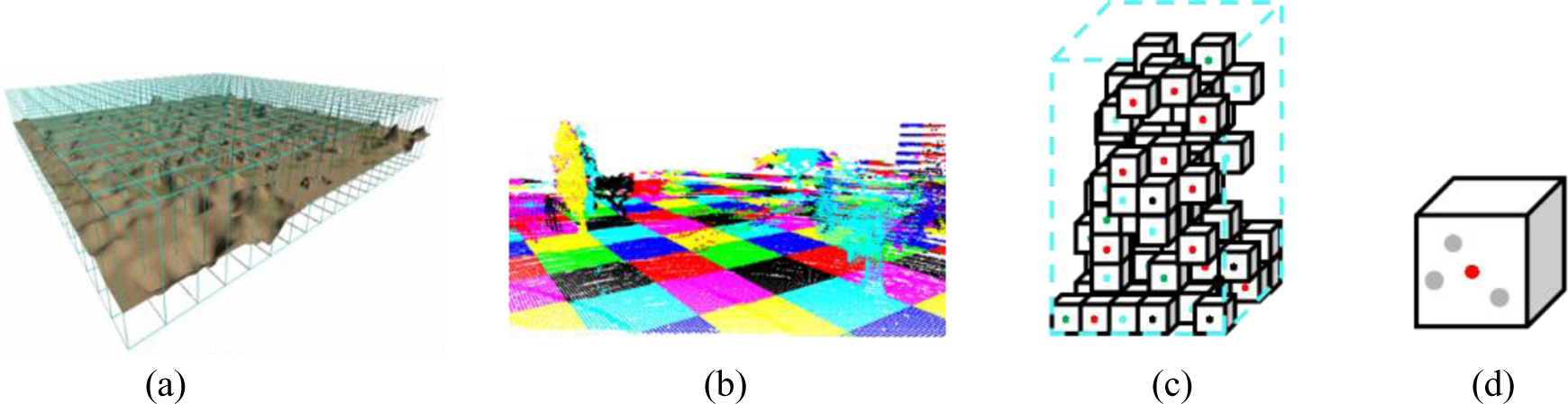
Concept of hierarchical voxel space: (a) illustrates the concept of segmenting the entire space into cells (world space); (b) presents each cell, configuring the cumulative voxel map in diverse colours (voxel map); (c) explains that raw points acquired through several frames accumulate scanned voxels, and the colour of the point in each voxel indicates the time when voxels are accumulated (cell); (d) indicates a voxel where a raw point is scanned and the grey point is the raw point scanned in a voxel space (scanned voxel).

Definition of dynamic object features in a cumulative voxel map

This article defines the features observed in cells with dynamic objects using the distribution of voxels accumulated in a cell. Since the location of an object changes whenever a sensor scans for dynamic objects, the location of a voxel where a raw point is scanned is different for each frame. Voxels accumulate for each frame, and the cumulative voxel group in a cell with a dynamic object indicates the movement trace of an object. Such a voxel is defined as a trace voxel. Figure 2 illustrates the concept of a trace voxel.

Figure 2.

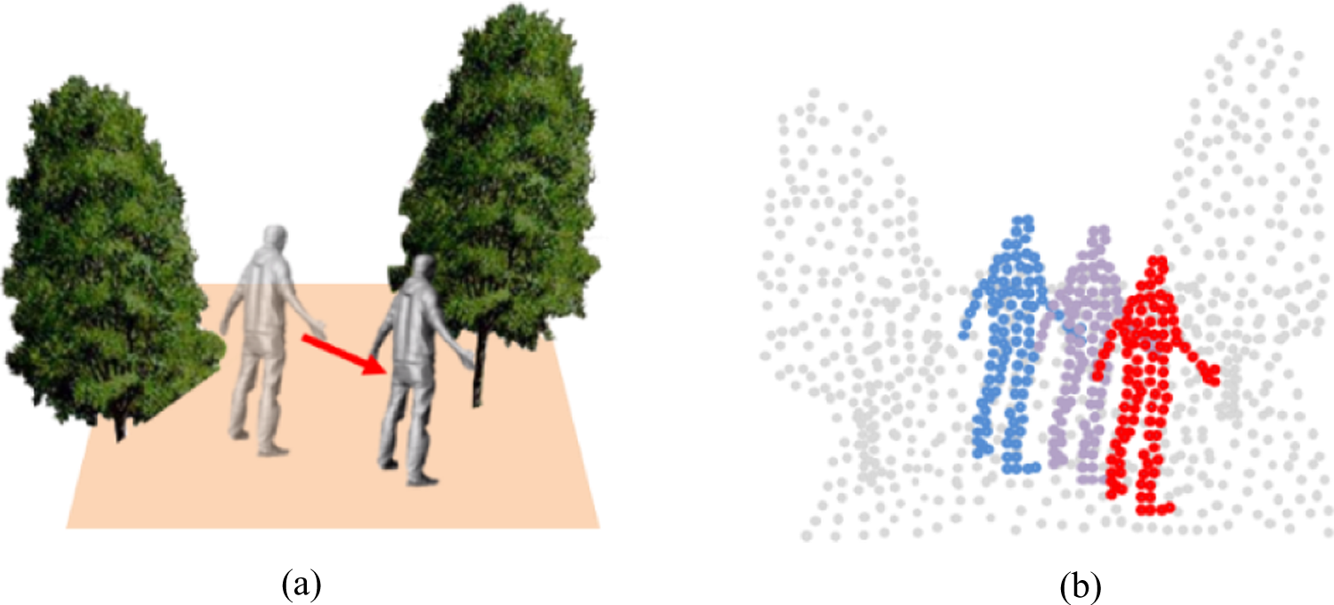
Trace voxels generated by a dynamic object: (a) an object moves and (b) cumulative voxels. When accumulating the voxels scanned for each frame as a human being moves, as shown in (a), the pattern illustrated in (b) is acquired.

This article categorizes the features of cells with dynamic objects into three types as follows: geometric changes, changes of cumulative voxel height in a cell and duplicate voxel distribution in accordance with the trace voxel of a dynamic object.

Geometric changes in a cell

When only static objects exist in a cell, the geometric shape formed by the voxel group is constant even when accumulating the voxels. On the contrary, cells with dynamic objects show changes of geometric shape formed by voxel groups due to the trace voxel of a dynamic object as voxels are gradually accumulated.

Figure 3 illustrates the geometric shape formed by a voxel group in a cumulative voxel map.

Figure 3.

Cumulative voxel maps including a dynamic object: accumulated (a) 2-frame, (b) 4-frame, (c) 6-frame and (d) 11-frame data. The yellow zones are the voxel zones with dynamic objects. Even when several frames are accumulated in the static zone, except yellow zones, the geometric shape formed by the voxel group is constant. On the contrary, the geometric shape formed by a voxel group in the yellow zone is changed.

The formula used to estimate the features of a geometry-featured voxel presented by Choe et al. is applied to define the geometric shape of a cell caused by a trace voxel. Choe et al. estimated the features of a point-ness, horizontal surface-ness, vertical surface-ness and post-ness using the covariance matrix on raw data. ^14,15 This article estimates the geometric features of a cell by estimating the covariance matrix on the voxel scanned by a raw point, as shown in Figure 4. At this stage, the voxel redefines a point as a mass because it is a much bigger unit than a raw point.

Figure 4.

Geometric features of a cell.

The value of each geometric feature is calculated using following equations

$f_{\text{Mass}}=c_{\text{Mass}}{\lambda }_3$

$f_{\text{HSuf}}=c_{\text{HSuf}}\left|{\left[\left({\lambda }_1-{\lambda }_3\right)\overrightarrow{e_1}\times \left({\lambda }_2-{\lambda }_3\right)\overrightarrow{e_2}\right]}^T\overrightarrow{y}\right|$

$f_{\text{VSuf}}=c_{\text{VSuf}}\left|{\left[\left({\lambda }_1-{\lambda }_3\right)\overrightarrow{e_1}\times \left({\lambda }_2-{\lambda }_3\right)\overrightarrow{e_2}\right]}^T\left(\overrightarrow{x}+\overrightarrow{z}\right)\right|$

$f_{\text{Post}}=c_{\text{Post}}\left|{\lambda }_1{\overrightarrow{e}}_1^T\right|-\left|{\left({\lambda }_2{\overrightarrow{e}}_2\times {\lambda }_3{\overrightarrow{e}}_3\right)}^T\overrightarrow{y}\right|$

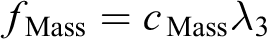
Each value represents how the points in a cell are distributed as each geometric feature. For an instance, the more the distribution of points in a cell appears similar to a horizontal surface, the higher the value of f _Mass.

Since only cells with static objects keep a constant shape for a voxel group accumulated in a cell, the geometric feature value of the present frame is not changed significantly from the previous frame. However, cells with dynamic objects have significant changes in geometric feature values because the shape of the voxel group is changed owing to the trace voxel of a dynamic object.

In particular, the trace voxel of a dynamic object gradually shows a dispersed shape as several frames are accumulated. Thus, mainly the mass feature increases among the geometric features of a cell. Figure 5 depicts a trace voxel significantly increasing the mass feature.

Figure 5.

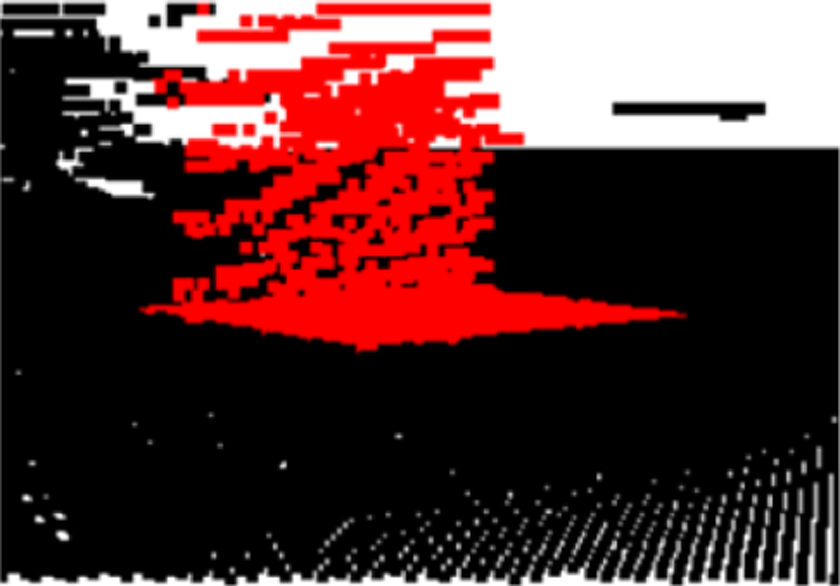
Mass feature represented by trace voxels.

Change of cumulative voxel height

When only static objects exist in a cell, all objects do not move. Accordingly, the height of a voxel configuring the relevant cell is always constant. On the contrary, when a cell includes dynamic objects, the trace voxel of a dynamic object is accumulated in the space where an object moves. In that case, the voxel height is changed.

Figure 6 describes a change of voxel height due to the objects in the cumulative space.

Figure 6.

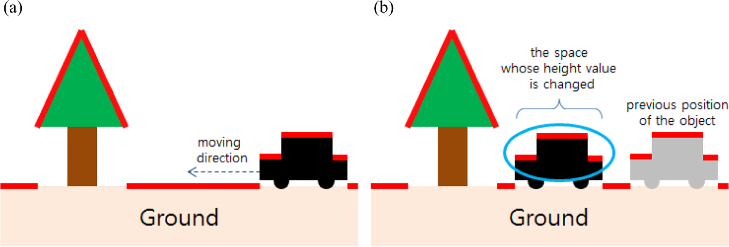
Change of voxel height due to presence of a dynamic object: (a) illustrates the initial status without movement of a dynamic object, and the height of each object is indicated in red (before an object moves); (b) presents the status of a dynamic object after movement. The height of the space where a dynamic object moved (yellow zone) has increased from the existing ground level to the height of an object (after the object has moved).

Duplicate voxel distribution

A duplicate voxel indicates a voxel space where the raw point of the present frame is scanned in duplicate in a voxel space where a raw point was scanned in the previous frame. While several duplicate voxels exist in a static object, there are almost no duplicate voxels among the trace voxels of dynamic objects. Figure 7 explains the distribution of duplicate voxels in the dynamic zone and the static zone.

Figure 7.

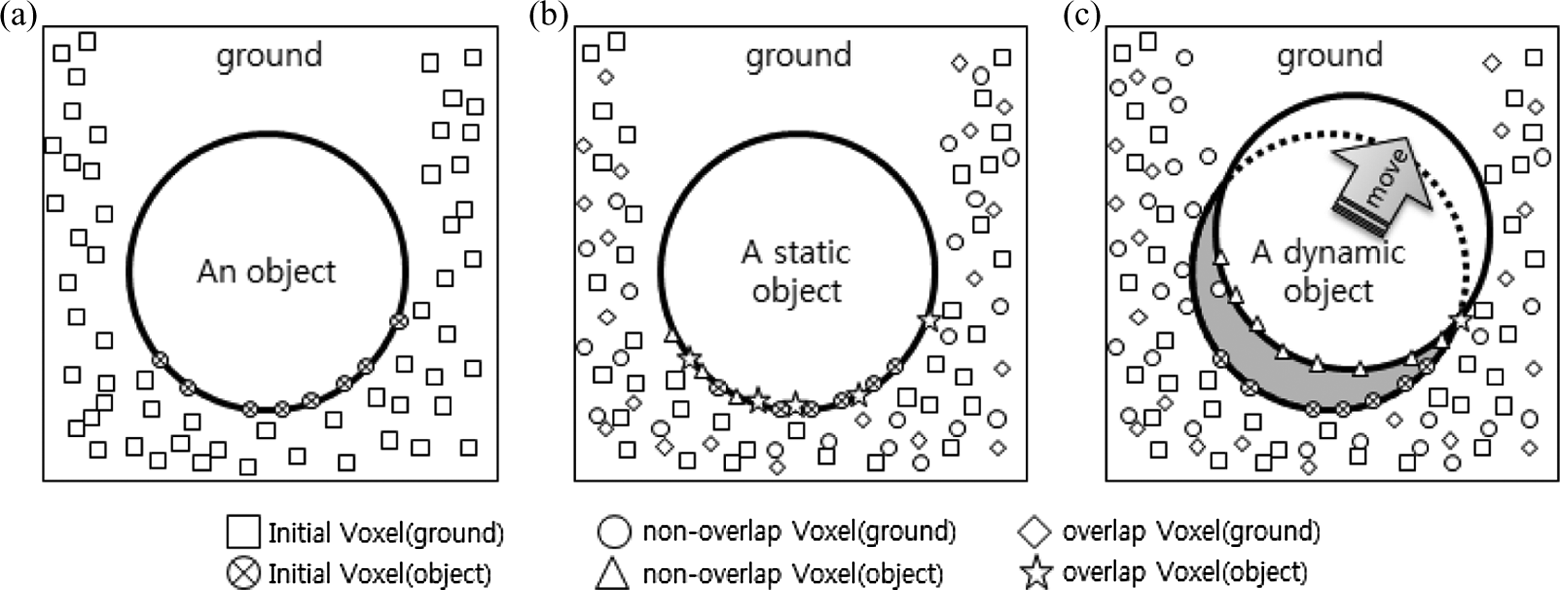
Distribution of duplicate voxels in cases of static and dynamic objects: (a) presents the results from the first scanning of a cylindrically shaped object and the ground (initial state). The green points are voxels scanned in the cylindrical zone and the purple points are voxels scanned in the ground zone. (b) Illustrates the result in second frame when the cylindrical object is static (overlap voxel state for static object). (c) Explains the result in second frame when the cylindrical object is dynamic (overlap voxel state for dynamic object).

When the cylindrical object is static, it exists in the same location even in the next frame. At this point, the scan result shows the same shape as shown in Figure 7(b). The red points are voxels newly scanned in the ground zone, and the blue points are duplicate voxels scanned in the ground zone. The sky-blue points are new scanned voxels against the object, and the yellow points are duplicate scanned voxels against the object. On the contrary, when the cylindrical object is dynamic, the scan result is the same as shown in Figure 7(c). The colour scheme for the points is the same as that in Figure 7(b).

Dynamic zone detection algorithm

A three-pass algorithm is proposed to estimate zones with dynamic objects using the three features described above. The estimation of geometric features of a cell enables quickly estimating the dynamic zone because it does not compare the locational correlation of cumulative voxels between the present and the previous frames. On the contrary, the estimation of duplicate voxel distribution and change of cumulative voxel height, which requires comparison of voxels between the present frame and the previous frame, have a slower processing rate than the estimation of the geometric features of a cell. Hence, the dynamic zone is estimated using the geometric feature changes of a cell. Next, the static zones miscalculated in the dynamic zone are eliminated using the change of cumulative voxel height and the distribution of duplicate voxels.

Dynamic zone estimation

A cell is estimated as being in the dynamic zone using the change of geometric features of a cell as described below. When the increase of a mass feature as compared to the previous frame is larger than a specific threshold, the relevant cell is estimated as being inside the dynamic zone. This is because the trace voxel of a dynamic object has a significantly larger mass feature. Next, when the total change of the four geometric features of a cell is larger than the threshold as compared to the previous frame, the cell is determined as being inside the dynamic zone. This considers the general impact of the trace shape of a dynamic object on other geometric features as well as mass.

However, the geometric features of a cell are significantly changed in some cases even though there is no dynamic object because the sensor platform moves with each frame. For instance, an object hidden by another object at close range in the previous frame can be observed in the next frame after the movement of a sensor. In addition, only one side of a specific object may be observed in the previous frame while other sides of the object are observed in the next frame after movement of a sensor.

Such events occur frequently in environments with objects, whose tops are larger than their bottoms, such as trees. Figure 8 represents the change of geometric features due to vehicle movement.

Figure 8.

Change of geometric features due to vehicle movement: (a) shows the zone scanned when a sensor moves in areas with a number of trees (environment) and (b) shows the zone scanned at the initial location of a sensor (initial state (t ₀)). The grey points indicate the points scanned. (c) Presents the zone scanned after the movement of a sensor, and the red points indicate the points scanned after movement (after car move (t ₁)).

The blue and red ground zones behind the tree close to the sensor are scanned at the initial position. After the sensor is moved, the yellow and purple zones, which cannot be scanned at the initial position, are scanned. The red and blue zones are the ground zones and so show more significant horizontal surface features. However, the yellow and purple zones scanned after the movement of the sensor have a significant change of geometric features in a cell because of significant mass and post-features.

For solving such issues, this article estimates the geometric features of a cell using only the voxel of the bottom of an object. The dynamic zone can be estimated because the mass feature value is increased due to the trace voxel of the dynamic object, even without reflecting the features of the top part of an object, because the dynamic object moves while keeping a short distance from the ground.

Accordingly, the feature value is estimated using the voxel within the offset height from the minimum voxel height in a cell in the process used to estimate the geometric features of a cell. Algorithm 1 describes the process used to estimate a dynamic zone using the change of geometric features of a cell in pseudocode.

Algorithm 1.

Estimation of dynamic object cells based on changes of geometric features.

Input: cellList // input list of cells

Output: dynamicZone // estimated list of dynamic object cells

Parameter: height_offset, mass_threshold, total_threshold // thresholds of geometric features

Start

1 dynamicZone = {};

2 For each cell ∈ cellList do

3 {

4  // find valid voxels in previous and current frames

5  prev_targetVoxelList ← cell.FindTargetVoxel    (cell.prev_VoxelList, height_offset);

6  current_targetVoxelList ← cell.FindTargetVoxel    (cell.current_VoxelList, height_offset);

7  // calculate geometric feature value for each valid voxel    in previous and current frames

8  prev_feature ← ExtractFeature(prev_targetVoxelList);

9  current_feature ← ExtractFeature(current_target    VoxelList);

10 // estimate dynamic object cell based on the change of    geometric features

11 mass_variation = current_feature.mass - prev_    feature.mass;

12 total_vatiation = Sum_variation(current_feature, prev_    feature);

13 If(mass_variation > mass_threshold or total_vatiation >    total_threshold)

dynamicZone = dynamicZone ∪ cell;

14 }

End

Fine tuning of estimated dynamic object cells

This article determines the cells without any change of cumulative voxel height as being included to the static zone and eliminates them from the estimated dynamic zone. The changes of cumulative voxel height in a cell are detected using the difference image of the cumulative voxel height map, which is a data structure of 2D coordinates where the value of each coordinate is the height of a voxel. Let us use the axis z in the voxel space in a cell as the height axis. The height of the highest voxel among voxels having the same (x, y) coordinates in the same voxel map in a cell is assigned to each (x, y) coordinate in the cumulative voxel height map.

However, since LIDAR sensors have low vertical resolution, no voxel is scanned at a specific set of (x, y) coordinates, but a voxel is scanned at the same coordinates in the next frame in some cases. This kind of event leads to the case in which there are no height values in the cumulative voxel height map in a frame, but the coordinates with height values are identified in the cumulative voxel height map of the next frame. This is the reason that a difference image with a change of height can be generated even without any actual change of height when generating the difference image between two voxel height maps.

To solve the problem above, a binary mask is generated for coordinates having the height value on the cumulative voxel height map in the previous frame. The difference image is only applied to coordinates where the height value in the previous image is generated for the relevant mask. When the number of coordinates with the change of height in the difference image applying the binary mask is smaller than the threshold, the relevant cell is eliminated from the dynamic zone. Algorithm 2 presents the pseudocode describing the process to eliminate the static zone on the basis of cumulative voxel height change.

Algorithm 2.

Removal of static object cells based on cumulative voxel maps.

Input: dynamicZone // estimated list of dynamic object cells

Output: dynamicZone // fine-tuned list of dynamic object cells

Parameter: threshold // threshold to differentiate static and dynamic object cells

Start

1 staticZone= {};

2 For each cell ∈ dynamicZone do

3 {

4  // generate 2D heightmap for previous and current    frames

5  prev_voxel_heightmap ← GenerateVoxelHeightmap    (cell.prev_VoxelList);

6  current_voxel_heightmap ← GenerateVoxelHeightmap    (cell.current_VoxelList);

7  // generate binary mask to tell Subtract() which    coordinate is valid

8  binary_mask ← GenerateBinaryMask(prev_voxel_    heightmap);

9  // calculate difference image

10 subtract_Image ← Subtract(current_voxel_heightmap,    prev_voxel_heightmap, binary_mask);

11 // estimate whether each cell is static

12 higherVoxelCount = GetChangedHeightCount    (subtract_Image);

13 if(higherVoxelCount < threshold)

staticZone = staticZone ∪ cell;

14 }

15 // remove estimated static zone from dynamic zone

16 dynamicZone = dynamicZone – staticZone;

End

Finally, the static zone is eliminated from the dynamic zone estimated on the basis of the duplicate voxel distribution. To this end, duplicate voxels are identified in the previous and present frames. Next, the duplicate voxels against an object are selected from among the duplicate voxels. When the ratio of duplicate voxels containing an object to the total number of duplicate voxels is higher than the threshold, the relevant cell is eliminated from the dynamic zone. This article estimates the duplicate voxels against an object as duplicate voxels located higher than ground voxels by considering that objects are above the ground in order to improve the processing rate. At this point, the ground voxels are estimated as the voxels below the average height of voxels in a cell. Algorithm 3 presents the pseudocode describing the process used to eliminate the static zone on the basis of the duplicate voxel distribution.

Algorithm 3.

Removal of static object cells based on the distribution of duplicate voxels.

Input: dynamicZone // estimated list of dynamic object cells

Output: dynamicZone // fine-tuned list of dynamic object cells

Parameter: threshold // threshold to differentiate static and dynamic object cells

Start

1 staticZone = {};

2 // calculate average height for all

3 average_height = CalculateAverageVoxelHeight    (cell.current_VoxelList);

4

5 For each cell ∈ dynamicZone do

6 {

7  // find voxels which exists both previous and current frames

8  overlapVoxelList←FindOverlapVoxels(cell.prev_VoxelList,    cell.current_VoxelList);

9  // select objects voxels from overlapped voxels

10 object_ overlapVoxelList ← SelectObjectOverlapVoxel    (average_height);

11 // calculate how many object voxels exist in each cell

12 object_overlap_ratio = object_ overlapVoxelList.count /   overlapVoxelList.count;

13 // estimate whether each cell is static

14 if(object_overlap_ratio > threshold)

staticZone = staticZone ∪ cell;

15 }

16 // remove estimated static zone from dynamic zone

17 dynamicZone = dynamicZone – staticZone;

End

Experiment and analysis

This section describes the experiment used to investigate the performance of the proposed approach for detecting the dynamic zone. First, the experimental environment and data set applied in the experiment are described. Next, the detection result of the dynamic zone estimated using the proposed approach is presented, and its performance is analysed.

Experimental environment

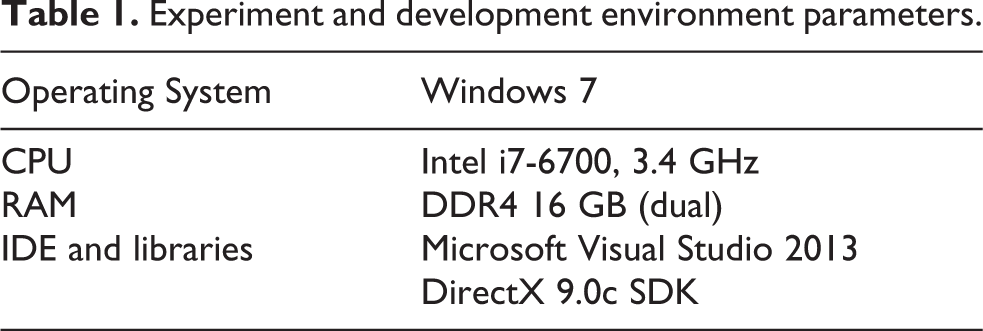
This article produced a 3D voxel visualization programme for use in the experiment. The detection result for a dynamic zone is visualized using the relevant programme, and the accuracy is estimated on the basis of the ground truth data set, which is generated by LIDAR simulator. The produced programme comprises a preprocessing module for generating voxels and segmenting cells, a module to estimate the dynamic zone using the change of geometric features of a cell, a post-processing module to eliminate static zones misjudged using the duplicate voxel distribution and change of cumulative voxel height and a module to visualize voxel points. Figure 9 illustrates the structure of the programme applied in the experiment, and Table 1 describes the specifications of the computer used for programme development and in the experiment.

Figure 9.

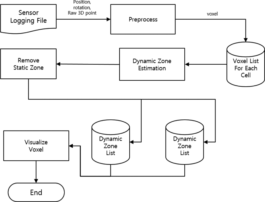
Structure of the experimental application.

Table 1.

Experiment and development environment parameters.

Operating System	Windows 7
CPU	Intel i7-6700, 3.4 GHz
RAM	DDR4 16 GB (dual)
IDE and libraries	Microsoft Visual Studio 2013 DirectX 9.0c SDK

Two kinds of data were used: a ground truth data set generated by an LIDAR simulator and a real data set. The simulator generated data using a virtual sensor platform controlled by user input in a virtual environment comprising geography, trees, human beings and vehicles. ¹⁶ The environment scanned through simulation is presented in Figure 10.

Figure 10.

Virtual simulation environment. The blue arrow indicates the movement of the sensor platform. Vehicle #1 and human beings #1 and #2 move in the direction shown by each arrow as soon as the simulation starts, and then stop. Vehicle #2 does not move at first, but starts moving after a certain period.

The environment of the real data set includes a vehicle utilizing inertial measurement unit-global positioning system and Velodyne HDL-32E LIDAR with small remote-controlled carts arranged around the vehicle. Figure 11 shows a photo of the surrounding environment where the experiment was executed along with the dynamic object.

Figure 11.

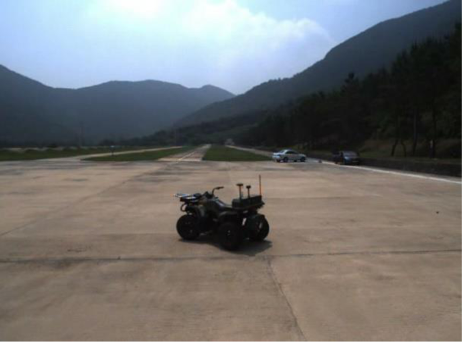
Real data set environment.

Experimental results and analysis

This section analyses the accuracy and processing rate of the approach estimating the existence of dynamic objects on the basis of ground truth data and explains the estimation results in dynamic zones using the proposed approach with actual sensor data.

The image on the left in Figure 12 is the sensor data logging environment of the simulator and that on the right indicates the estimation results by comparison with ground truth data.

Figure 12.

Estimation result based on the ground truth data set. The blue cells in the right image in (a) to (d) accurately estimated the zones with dynamic objects. The green cells were not estimated as dynamic zones but were close to blue cells. The red cell contained dynamic objects but was estimated as a static zone with all its neighbouring cells. The sky-blue cells are estimated as dynamic zones that are static zones in the ground truth data.

There are three reasons for false negatives, which are failures to detect zones with dynamic objects in the experiment. First, the dynamic object at a distance was hidden behind a specific object in front of it, and so only a few voxels were scanned. The relevant zones were estimated as static zones because there were not sufficient voxels to judge the cell as containing dynamic objects. Figure 12(a) presents false negatives in which cells including human being #2 at a distance were judged as being inside the static zone.

Second, when a dynamic object that did not initially move at a distance later started moving, the status of the object, which was dynamically changed for about three frames, was not detected. This is the limit of the approach proposed in this article for estimating the dynamic object cells on the basis of cumulative voxels. Thus, it requires further investigation. Figure 12(c) explains that vehicle #2 at a distance started moving, but the cell including it was determined to be inside a static zone.

Third, when a dynamic object was on the edge of a cell, the voxels on that dynamic object were separated over several neighbouring cells, and so the number of voxels was not enough to implement the estimation for dynamic objects in those cells. Figure 13 illustrates a false negative (green) caused as the voxels on a dynamic object are dispersed over several cells.

Figure 13.

Estimation of neighbouring positive cells based on a dynamic object distributed over several cells.

However, when one of the cells with the dispersed voxels of a dynamic object is estimated as being inside the dynamic zone, it is classified as a neighbouring positive cell (green cell). Because the approach uses preprocessing to detect dynamic zones, clustering is executed with neighbouring positive cells, not only blue cells.

Table 2 illustrates the results of the proposed algorithm and the kinds of cells existing in ground truth data. The total cell count is the number of cells that had more than one cumulative voxel in 143 frames. The static object cell count is the number of cells without dynamic objects in the ground truth data. The dynamic object cell count is the number of cells with dynamic objects in the ground truth data. The false positive cell count is the number of cells that were judged as dynamic object cells although they did not contain dynamic objects. The false negative cell count is the number of cells that were judged as static object cells although they contain dynamic objects. The neighbouring positive cell count is the number of cells corresponding to neighbouring positive cells among the false negative cells.

Table 2.

Numeric performance results.

Total cell count	Static object cell count	Dynamic object cell count	False negative cell count	False positive cell count	Neighbouring positive cell count
39,297	38,864	433	136	110	110

Ratio_Dynamic-Hit and Ratio_Static-Hit are calculated to determine the detection accuracy of dynamic object cells. Ratio_Dynamic-Hit indicates the accuracy of estimating cells as dynamic object cells. Ratio_Static-Hit indicates the accuracy of estimating cells as the static object cells. Formula 1 is used to estimate each accuracy above. Table 3 shows the calculation results using formula 1

$\begin{array}{c}{\text{Ratio}}_{\text{Dynamic-Hit}}=1-\frac{\text{False\_negative}-\text{Neighbouring\_positive}}{\text{Dynamic}}\times 100\text{\%}\\ {\text{Ratio}}_{\text{Static-Hit}}=1-\frac{\text{False\_positive}}{\text{Static}}\times 100\text{\%}\end{array}$

1

Table 3.

Accuracy of dynamic object cell detection.

Detection accuracy		Processing time per frame
RatioDynamic-Hit	RatioStatic-Hit	Average	Deviation
93.99%	99.65%	18.38 (ms)	7.13

Figure 14 presents the experimental result from the estimation of dynamic objects using actual sensor data. However, with actual sensor data, there were several errors misjudging some static object cells as dynamic object cells due to the navigation data errors when a vehicle rapidly made a turn and due to noise from the LIDAR sensor.

Figure 14.

Experimental results using the real data set. The part figures (a) and (b) show good results, (c) shows false positives due to noise and (d) shows false positives due to IMU errors when the sensor platform turns rapidly.

We introduced only visual errors for real data set. To verify the quantitative accuracy of the proposed method, we are scheduled to make ground truth information of several real data sets.

Conclusion

This article proposed a preprocessing method for detecting zones containing dynamic objects in a cumulative voxel environment. This article estimated zones with dynamic objects by identifying the features of voxels corresponding to the traces made by dynamic objects in a cumulative voxel environment without segmenting the ground and objects. To this end, raw points were converted into voxels and accumulated, and the cumulative voxel map distributed over cells was implemented. Next, the dynamic object cells were estimated using the voxel distribution in each cell. Finally, the accuracy of the proposed approach was improved by post-processing, which eliminated the static object cells from the estimated dynamic object cells.

In accordance with the experimental results, the dynamic object cells were detected with an accuracy of 93.99%. The detection rate for one frame was 19 ms. Since the data acquisition cycle of LIDAR used in the experiment was 100 ms, it was verified that the approach proposed in this article could detect dynamic object cells in real time. The approach proposed in this article contributes significantly to reducing the processing time in efforts to detect dynamic objects using 3D LIDAR data.

For robustness, we are planning to enhance accuracy of our method, especially when the state of an object is changed from static to dynamic and vice versa, when a moving object is partially occluded by other objects and when a point cloud of moving object is divided by several cells. Furthermore, we captured more sensor data sets in various real environments, which have sensor errors and noises, to study the elimination of false positive cells and use same threshold for those data sets. To evaluate our method confidently in real environments, we need to generate ground truth information of the data sets in future.