
Abstract
Many works in the literature have studied the kinematical and dynamical issues of parallel robots. But it is still difficult to extend the vast control strategies to parallel mechanisms due to the complexity of the model-based control. This complexity is mainly caused by the presence of multiple closed kinematic chains, making the system naturally described by a set of differential–algebraic equations. The aim of this work is to control a two-degree-of-freedom parallel manipulator. A mechanical model based on differential–algebraic equations is given. The goal is to use the structural characteristics of the mechanical system to reduce the complexity of the nonlinear model. Therefore, a trajectory tracking control is achieved using the Takagi-Sugeno fuzzy model derived from the differential–algebraic equation forms and its linear matrix inequality constraints formulation. Simulation results show that the proposed approach based on differential–algebraic equations and Takagi-Sugeno fuzzy modeling leads to a better robustness against the structural uncertainties.
Keywords
Introduction
In modern societies, manipulators have become a key tool in industry due to their great versatility in repetitive task. The mechanical architectures traditionally used in automated production line are based on serial robots. These robots are made of a sequence of rigid links serially assembled through revolute and/or prismatic active joints. 1 In other words, the end effector is connected to the base via a single open-loop kinematic chain which gives them a large work space and high dexterity. 2 Despite these advantages, serial robot suffer from high inertia due to the position of actuators, which are located on the moving part, they also suffer from a low payload to weight ratio and a low precision due to the cumulative joint errors and link deflection. Owing to the drawback of serial robot, parallel manipulators have taken a great interest in many applications, such as high-speed machining, assembly and packaging task, flight simulators, and various medical and space applications. 3 –7 Parallel robots are generally characterized by their nonanthropomorphic shape, they are composed of an end effector connected to a base by at least two separate and independent kinematic chain. 8 This multiple kinematic chain provides a high rigidity and agility with a high payload to weight ratio due to the deportation of the actuators to the base and the distribution of the load between different chain. 9 However, they suffer from some drawbacks such as limited work space, abundance of singularities, 10 and complex dynamic model caused by the presence of multiple closed kinematic chains (CKCs). 11
Many works discussed the kinematic or the dynamic issues of CKCs. 9,12 But it is still relatively difficult to extend the vast control theory developed for serial manipulator to the parallel one, and this difficulty is due to the complexity of the model-based control. 13 This complexity comes from the fact that parallel robot are described by a set of differential–algebraic equations (DAEs) of index-3. 14 This differential index represents the number of time differentiating the constraint equations to obtain a set of ordinary differential equations (ODEs). 15 The main difficulty here is the high differential index (index > 2). 16,17 This makes the DAEs not explicitly expressed in the state–space representation which is a suitable form for most of the control strategies.
In the case where the model of the robot is given on the ODEs form, the simplest way for the control is the famous linear single-axis proportional integral derivative (PID) controller in the joints space. 8,18 –22 This method is well-known for its effectiveness under the assumption of locally linear dynamics. It is verified only for low-speed control and cannot be efficient over the whole work space with a single tuning. 23 An equivalent version of linear single-axis control in the Cartesian space is given in the works by Callegari and colleagues. 24 –27 In this case many simplifications are assumed that leads to a lack of accuracy and stability. 27 Another famous approach based on feedback linearization is the computed torque control (CTC). 28 This technique is widely spread in serial robotics 8,29,30 and has been implemented on several parallel platforms. 23,31 From this, the literature on the control of parallel robot based on ODE models is very large and mainly depends on the complexity of the studied manipulator and the targeted control strategy such as the sliding mode control, 32,33 the H∞ control, 34,35 the robust TS control, 3 the adaptive control, 36,37 the passivity-based approach, 38 and other variances. 10,23,39 –43 Despite this nonexhaustive scope, models of CKCs are still complex and highly nonlinear in most cases which makes the guarantee of stability in the Lyapunov sense quite difficult.
The aim of this work is to deal with the parallel robot on its DAE form, the difficulty here is that the DAE forms are not expressed explicitly in state–space representation. 44 From this, in the second section a DAE model is presented, then the ODE model is deduced to show how complex the ODE model could be. After that, a technique based on the input–output linearization (IOL) is used to write the DAEs model on the state–space representations with an algebraic equation helping to compute the nonlinear parameters that represent the internal forces of the robots. The originality here is that by computing the internal forces the robot can be fully described by two decoupled submodel and then, depending on the complexity of those models, the robot can be controlled either in the joints space or in the operational space. In the third section, a brief description of the Takagi-Sugeno (TS) modeling and control is given. The TS modeling is applied on the legs model of 2-degree-of-freedom (DOF) parallel manipulator by transforming the internal forces as premises for the control law. The interest of bonding the internal forces is to make the system naturally robust against the structured uncertainties just by solving some simple linear matrix inequality (LMI). In the last sections, a comparison between PDC and CTC control laws is presented and some concluding remarks are given.
Mechanical modeling of a 2-DOF parallel manipulator
DAE model of Biglide
The Biglide is a 2-DOF planar parallel manipulator
31,45
(Figure 1). This parallel kinematic machine consists of two bars mounted through a joint on two separate sliding blocks (active prismatic joints), the extremity of each bar is connected to an end effector, thereby forming a CKC. This configuration allows the positioning of the end effector (operational coordinates:

Kinematic diagram of Biglide robot.
The kinematic analysis of the Biglide leads to the following constraint of loop closure

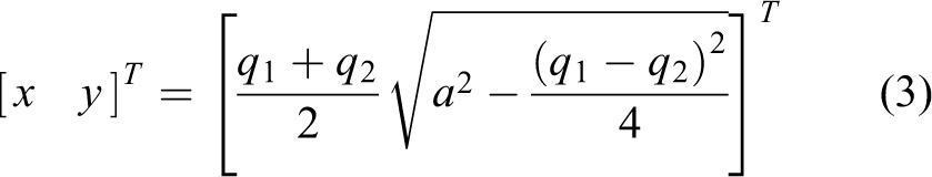
The inverse kinematics can thereby be expressed as

Thanks to its simple mechanism, the forward kinematics of the Biglide can be easily derived from equation (2)
Under the assumption that the mechanical system satisfies the loop-closure constraint, the kinematic relationship between end effector velocities and active joints velocities is computed by differentiating the constraint (1) with respect to time, and this relationship is conveniently described by two Jacobian matrices

with
In order to derive motion equations of the Biglide, the structural characteristics of the robot are exploited to write a model based on two independent subsystems: the end effector dynamics and the open-kinematic chains dynamics. The actuator forces (robot inputs) are denoted by


where
With m, mi , msi , Ji , i = 1,2 are the inertial parameters of the robot, which are the end effector mass, the mass, and the first and second moments of link i related to revolute joint axis on the sliding blocks 1 and 2, respectively.
From the kinematic constraint it is easy to write passive joints coordinate functions of operational coordinates.

Thereby, the velocities of passive joints can be expressed as
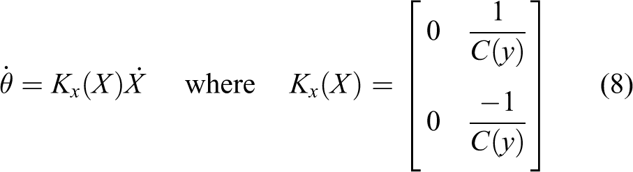
Using the equations (7) and(8), the dynamic of the open-kinematic chain Hi , i = {1,2} given by equation (5) are reordered into active part Hq and passive part Hθ such that

with M
11 = diag(m
1, m
2),
The virtual power

Using equation (8), the virtual passive velocities is eliminated with

The new virtual velocities field

Finally, the virtual power with the Lagrange multipliers is expressed as follows

Given that the Lagrange multipliers are unknown, the virtual velocities field
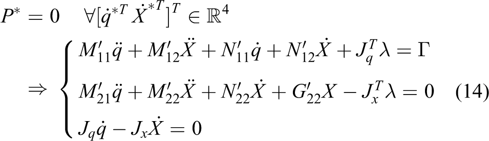
with
Input–output linearization
The DAEs model given by equation (14), presents the coupled dynamics between the legs and the end effector. The algebraic variables (Lagrange multipliers λi) represent the internal forces between the legs and the end effector. The assembly of the two subsystems is ensured through the algebraic constraint. This model is singular, the difficulty here is that DAEs are not expressed explicitly in state–space representation. 44 From this, two main approaches have been developed. The first one is the approximation of the DAE model to a singularly perturbed model. 47 The idea is to substitute the constraint equation with a fast dynamics representing the violation of the constraint. 44,48 –50 From a practical point of view, this approach is completely justified because the connections between joints and links are elastic. 51 This method helps to relax the complexity of the nonlinear model through the additional artificial dynamics, but at the same time it extends the state vector. This leads to an increase in the complexity of the control applications based on the resolution of the LMI problem. The second technique is the IOL, 52 and this approach consists of solving the algebraic equation by differentiating the constraint until the appearance of the algebraic variables. The solution is used in the differential equation of the DAE system and a state–space model-based control is given. The differentiation of the constraint (14) is written as

By combining (15) with the DAEs model (14), a redundant ODEs model is obtained:

with
From system of equations (16) and by placing the differential equations into the algebraic one, the Biglide parallel robot can be fully described by two different subsystems as follows


with
This is the first main results of this article, the Biglide robot can be controlled by two different approaches depending on the targeted control law. The first approach is to only use the legs model equation (17). In this case, the internal forces λ are seen as nonlinear terms to be compensated by the controller. The second approach is to only consider the end effector model (18). In this case, the internal forces of the system are seen as a new input control defined by the algebraic equation.
ODEs model of Biglide
In order to get the ODEs model of Biglide in operational space, the virtual active joint velocities are eliminated from the virtual power equation (11) using the equation (4),

Therefore, the ODEs model can be obtained from equation (19) as

with
In a more general case, it is not obvious to get the ODEs model of parallel robot in operational space. To get the model in the active joint space, the same logic is followed by eliminating the virtual operational velocities. Note that the ODEs model is given here just for a comparison purpose with the DAEs one. Unlike the DAEs model, where most of the nonlinear terms are hidden into the algebraic equation, the ODEs model presents a large number of nonlinear terms. For this reason, we thought that it will be better to use the DAEs model to design nonlinear controllers.
PDC fuzzy control
TS modeling
The TS fuzzy model is a mathematical representation of systems, it belongs to the quasi LPV family. 53 Inside a compact set of state variables, TS fuzzy model can represent exactly a nonlinear system by a collection of linear models weighted together by a nonlinear function issued from nonlinearities of the system. 54 The conditions of stability and stabilization of these models are generally based on the Lyapunov theory. 55 The advantage of this representation is that it provides a systematic framework for designing control laws through the LMI constrain formulation. 56
Let’s consider the following nonlinear plant
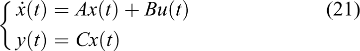
where
Let r be the number of nonlinear terms of the system (21). A TS model is viewed as a convex sum of linear models via membership functions (MFs), it is defined by «If…Then» rules representing the local linear input–output relations of the plant. 53 From this, the nonlinear system (21) can be written on continuous-time TS fuzzy model as follows 56

where z(t) is the premise vector (vector of nonlinear terms of the model). It may depend on the state, input, exogenous parameters, or time, on measurable and/or unmeasurable variables. Matrices (Ai
, Bi
),
TS model of the legs
For the following, let’s consider the dynamical model of the Biglide given by equation (17). In order to decompose the internal forces λ into a convex sum, the term

Then, the state–space representation of the Biglide robot in term of joint variables

where
From the state representation (24), the TS fuzzy model of the Biglide can be obtained by considering the following two nonlinearities

with
Controller design
For the stabilization of system (22), a parallel distributed compensation (PDC) control law is proposed 57

where the matrices

with
An integral part is added (Figure 2) in order to compensate the stationary error. Consider the extended state vector

Extended PDC control scheme.

where yd is the desired input vector. The extended system is expressed as

with

with the extended gain vector
Simulation results
The model of the parallel robot used for numerical simulations includes structured and unstructured uncertainties (Appendix 1). The structured uncertainties represent the variation in the end-effector mass, this variation is given by
In order to get the TS numerical model, the joint positions were bounded in a manner to avoid singularities and to cover a large area of the working space
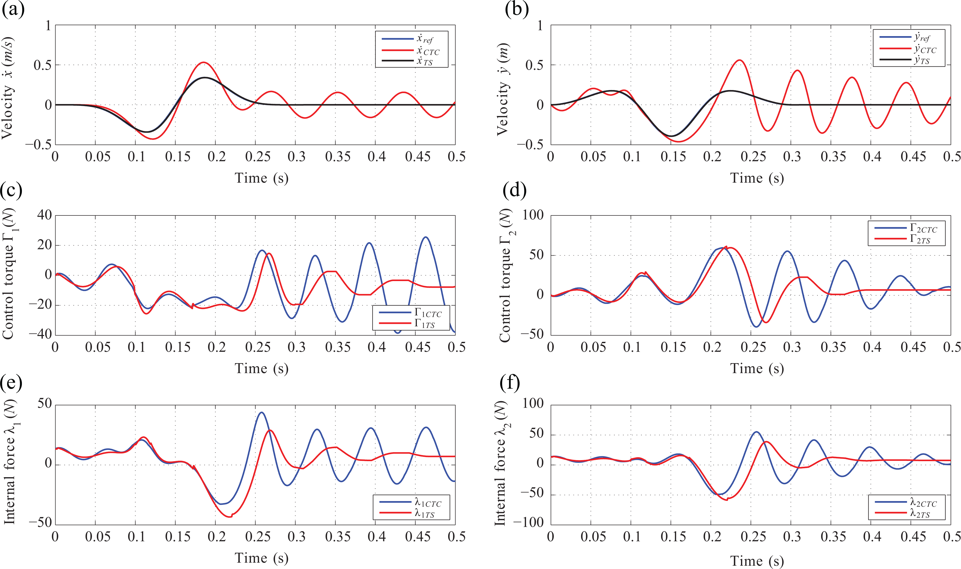
For the simulation, we chose a circular trajectory in the operational space. The response of both controllers, CTC and TS, are depicted in Figures 3 and 4 for the model without payload

Simulation results for

Simulation results for

Simulation results for

Simulation results for
Simulation results for

Simulation results for
In the case where the robot does not carry any payload, both control laws ensure a good tracking with a slight advantage to the TS control law, so we can say that the TS and CTC are robust against the unmodeled dynamics (stick/slip friction). Moreover, from Figure 3 (c and d) we can note that the control inputs are almost similar, this indicates that the two controllers were tuned in a manner to get similar performances in the nominal case. In the second case,
Finally, two well-known criteria are computed over the simulation time (T = 0.5 s) in order to quantify the behavior of both controllers (Table 1): the first criterion is the integral of absolute error:
ISV and IAE criteria.

ISV: integral of square value of the control; IAE: integral of absolute error; TS: Takagi-Sugeno; CTC: computed torque control.
Conclusion
This article proposes a novel approach for the control of parallel robots. Those systems are particularly difficult to control due to the presence of multiple CKCs. These mechanical loops lead to a model naturally described by a set of DAEs of index-3. Designing a controller based on the DAE model is not an easy task, it requires a particular knowledge on the control theory of singular systems. For this reason, most of the time we transform the DAE model into an ODE one by differentiating the constraint twice. This manipulation is appropriate for mechanical systems because if the system is well designed, the initial conditions should respect the algebraic constraint. Unfortunately, the obtained ODE model is most of the time complex and highly nonlinear. This makes the design of nonlinear controllers that requires the use of convex optimization techniques such as TS modeling and LMIs quite difficult. Because, in this case, the complexity of the controller is an exponential function of the number of nonlinear terms. For this reason, this article proposes to keep the DAE form of the system in order to decouple it into two independent subsystems. The idea here is to collect most of the nonlinear terms inside the Lagrange multipliers
Footnotes
Acknowledgement
This research was supported by International Campus on Safety and Intermodality in Transportation, the Nord/Pas-de-Calais Region, the European Community, the Regional Delegation for Research and Technology, the Ministry of Higher Education and Research, the French National Research Agency, the National Center for Scientific Research and the Arts Carnot Institute. The authors gratefully acknowledge the support of these institutions, in addition to all partners of the VHIPOD project (Self-balancing transport vehicle for handicapped person in standing position with support for verticalization, ref : ANR-12-TECS-0001) : Laboratory of Medical information Processing (LaTIM-INSERM UMR 1101), National Centre of Resources and Innovation with a mission to promote mobility for all persons at any age (CEREMH), Kerpape Mutualistic Functional Reeducation and Rehabilitation Center (CMRRF of Kerpape) and BA systmes corporation.
Declaration of conflicting interests
The author(s) declared no potential conflicts of interest with respect to the research, authorship, and/or publication of this article.
Funding
The author(s) received no financial support for the research, authorship, and/or publication of this article.
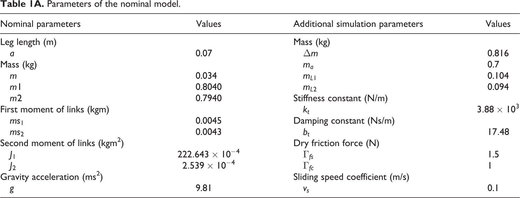
Appendix 1
Parameters of the nominal model.
| Nominal parameters | Values | Additional simulation parameters | Values |
|---|---|---|---|
| Leg length (m) | Mass (kg) | ||
| a | 0.07 | Δm | 0.816 |
| Mass (kg) | ma | 0.7 | |
| m | 0.034 | mL1 | 0.104 |
| m1 | 0.8040 | mL2 | 0.094 |
| m2 | 0.7940 | Stiffness constant (N/m) | |
| First moment of links (kgm) | kt | ||
| ms1 | 0.0045 | Damping constant (Ns/m) | |
| ms2 | 0.0043 | bt | 17.48 |
| Second moment of links (kgm2) | Dry friction force (N) | ||
| J1 | Γfs | 1.5 | |
| J2 | Γfc | 1 | |
| Gravity acceleration (ms2) | Sliding speed coefficient (m/s) | ||
| g | 9.81 | vs | 0.1 |