Sage Journals: Discover world-class research

Abstract

In order to improve the operational efficiency of robot-based shoe manufacturing, a method of shoe-groove tracking based on industrial robot is presented in the article. First, side surface of a shoe upper with a sole is scanned with a laser scanning device. The presented approach mainly consists of two steps: reconstruction of three-dimensional point cloud and feature curve extraction. It is difficult to extract the closed groove curve on shoe surface. We propose an innovative method to simplify the feature extraction through projecting geometric information from three dimension to two dimension, which is convenient to identify longest groove feature line in two-dimensional space. After detecting the two-dimensional groove line, we back project it to three-dimensional space to identify the three-dimensional thick groove point set. Finally, we thin and fit the groove curve into a trackable sequential curve. The experimental results show that the proposed system can effectively detect the shoe groove and generate trackable sequential curve. We also simulate the robot tracking process in a virtual environment to demonstrate the effectiveness of the presented method.

Keywords

Shoe manufacturing laser line sensor 3-D scanning shoe-groove feature robot tracking

Introduction

In the past decades, robot-based automation technologies have mainly been deployed in capital-intensive large volume manufacturing, such as in automobile, aircraft, electronics, and shipbuilding. For example, more than 60% of the total annual robots are employed in automotive and electronics industrial and their supply chains. In recent years, with the requirements of highest productivity and flexibility of the manufacturing equipment and higher labor cost, robot-related technologies have been utilized in small- and medium-sized manufacturing, such as food, logistics, recycling, and so on.

Shoe making is a very old and important technique for human being. The process of shoe making is usually complex and very time-consuming, including style and appearance designing, forming the last, patterning, closing, stretching, attaching, finishing, and so on. Each of them also contains many tiny steps to accomplish it. Cobblers in ancient times and some handicraftsmen today have to produce shoes entirely by hand, which does tend to be less precise and is often much more expensive.

Modern cobblers can depend on the help of a number of machines. In some instances, the entire manufacturing process can be more or less automated, which is often the case with many mass-market footwear choices. The automation process often brings the cost down, which allows manufacturers to make more and charge less for each pair. Even very expensive custom-built products often make use of some machine help, though, particularly when it comes to making precise cuts, stitching through tough material, and measuring patterns. Therefore, in shoe making industry, the robot-based automation can be deployed.

In the attachment procedure of shoe making, the cobbler actually bonds the upper and the sole together. This is often done with cobbler’s glue or another strong adhesive, but a lot depends on the type of shoe. Sometimes, bolts, screws, or stitches are better options. But for sport shoes, the glue or some other adhesive is a must for the characteristics of materials. Before attaching the upper with a sole, the bottom edge of the sole, called shoe groove, must be marked with a line and ground in order to keep consistency, spray glue, and increase the cohesion for leather or some other glossy upper material. Figure 1 shows two examples of marking line drawing by hand in shoe manufacturing. It needs a simple machine to make the line drawing ease. First, the worker puts a sole and an upper with a last B together on a turntable C, and using two sticks A pushes them tightly. Then, the turntable C is rotated by hand and a marking line is drawn using a pen.

Figure 1.

Drawing a line at the sole edge manually.

As aforementioned, in order to keep the sole consistent and strengthen the adhesion beneath, the shoe groove should be ground. Traditionally, this can be conducted manually. But at present, we can use a robot manipulator with a grinding wheel to accomplish it. Figure 2 is an example to grind the shoe groove with a robot.

Figure 2.

Grinding the shoe groove with a robot.

However, one of the issues of the robot-based grinding method is how to decide the trajectory for the robot according to the shoe groove. One method is to guide the robot to track the shoe groove. As shown in Figure 3, some key points are marked on the shoe groove to guide the robot to track each point and form a tracking trajectory. As we can see, this procedure is time-consuming and even not very accurate.

Figure 3.

Marking key points on the shoe groove by hand.

With the development of computer vision, we can use the vision system to guide the robot to find the trajectory, which can improve the effectiveness and automation. In this article, we propose a three-dimensional (3-D) vision system to find the shoe groove in shoe manufacturing. First, a structural laser–based 3-D scanning apparatus is used to acquire 3-D point set of a shoe. Second, the feature points are extracted from the point set based on a level-set method. Third, the 3-D feature points are projected onto a two-dimensional (2-D) plane space to extract the longest closed line of points, which is the corresponding shoe groove in 3-D space. Finally, the consequent upper with a last is scanned in assembly line and matched with the prescanned shoe model on the basis of iterative closest point (ICP) method. From the pre-extracted shoe groove and the normal of feature points, we can obtain new shoe groove on the upper, which can be used to guide the robot to grind, spray glue, and do some other operations. Figure 4 demonstrates the flowchart of our proposed shoe-groove extraction method.

Figure 4.

System flowchart of the trajectory tracking for shoe groove.

Related work

In general, methods of acquiring 3-D shape of a real object can be classified into two different groups: active methods and passive methods. The active method is to obtain precise 3-D data by laser range scanners or coded structured light projecting systems. Passive methods work in an ordinary environment with simple devices and flexibilities and provide feasible and comfortable means to extract 3-D information from a set of calibrated pictures. Although passive-based method is a convenient way to recover 3-D shape, but its accuracy is not adequate enough, and even worse, the computational speed cannot meet the requirement of real-time applications.

Laser-based 3-D scanning technology has lots of applications, such as in reverse engineering, robot navigation, historical relics and museum objects preservation, and terrestrial survey. Reverse engineering takes an existing product and creates a CAD model from 3-D scanning, for modification or reproduction to the design aspect of the product.^1,2 The laser-based 3-D measurement methods are commonly used in robotics, for instance, in navigation, grasping, and manipulation.

Blodow et al. propose a humanoid robot grasping system based on 3-D laser scans.³ In the presented sample consensus framework, cylinders, cones, and arbitrary rotational surfaces can be reliably and efficiently detected, and using the symmetry assumptions, the occluded parts of the object can be modeled from a single view. A portable 3-D laser scanning system with large depth-of-view has been designed and built for robot vision in the study of Li et al.⁴ Harrision and Newman proposed an end-to-end system capable of generating high-quality 3-D point clouds from the popular LMS200 laser on a continuously moving platform with more details.⁵

Fan et al. utilized a robot-based 3-D laser scanning system in which a structured light vision sensor is mounted on the six degree-of-freedom (6-DOF) robot to overcome the disadvantages of coordinate measuring machine.⁶ The hardware configuration in the study of Fan et al.⁶ is the same as that in our article, but the calibration and data processing are very different. An improved Tsai’s method and a multilayer perception neural network approach to calibrate the vision sensor are presented by using sufficient fiducial points generated from the robot. In our system, we use a ring pattern and Zhang’s method to calibrate the structured system. It is much simpler than the method of Fan et al.⁶

Laser scanners are capable of acquiring range measurements at rates of tens to hundreds of thousands of points per second, at distances of up to a few hundred meters, and with uncertainties on the scale of millimeters to a few centimeters. It is suitable for recovering the 3-D models of large-scale terrains, forests, large buildings, and so on.^7

–11 Capturing the historical heritage and cultural artifacts in their existing state is critical for their preservation, exhibition, and to gain in-depth knowledge. 3-D laser scanning is used to record cultural features rapidly and accurately despite the harsh conditions present at the site.¹² Huber et al. gave comprehensive survey of 3-D modeling and analysis in the architecture, engineering, and construction domain for developing modeling and recognition algorithms to support the automatic creation of building models from laser data.¹³

Besides the different applications of 3-D laser scanning, other aspects are how to improve the accuracy of the scanned data and how to register surface patches into a watertight model. Isheil et al. discussed the factors to influence the accuracy through an error correction procedure based on an experimental process that concerns mechanical parts.¹⁴ Chen et al. proposed the present Hong-Tan-based ICP automatic registration algorithm for partially overlapping range images for both smooth and high-noise range images.²⁸ Other work concerning laser scanning technologies involve system design,^15,16 data processing,¹⁷ and so on.

RGB-D sensors combine RGB color information with per-pixel depth information. New consumer RGB-D sensors cost less than US$200, such as Microsoft Kinect Redmond USA, Asus Xtion Pro Taibei, and Intel Realsense California, which can offer an affordable and easy method to acquire 3-D information. It can be utilized in some applications, such as 3-D mapping and simultaneous localization and mapping (SLAM),¹⁸ hand gesture or human pose recognition,¹⁹ sensing of the environment,²⁰ and so on. However, the 3-D surface reconstructed from RGD-D sensors has not enough accuracy.

As far as we know now, there is not an exact same system in literature used in shoe making industry. The Robofoot project offers a systematic solution for automatic shoe manufacturing.²¹ Although it has the functionality of polishing, inking, and gluing, it is not giving more technique details. The main difficulty of our approach is how to extract the closed shoe-groove line. There is not an off-the-shelf method to solve this problem well, although there are lots of methods to extract saliency, edge, or sharp features on a 3-D triangular mesh in computer graphics.^22
–24 In short, the main contributions of our article have two folds. One is the whole system to solve the problem of the shoe-groove extraction and tracking and another is the specific data processing of dimensionalities reduction to simplify the feature curve extraction in 2-D.

System design

Design of the scanning device

In order to scan the shoe upper, we design a scanning system as shown in Figure 5, left. It consists of an industrial camera A, a structural line laser emitter B, an indicator C, and a holder D with flange. This device is mounted on a UR robot with flange plate as in Figure 5, right. The direction of laser is perpendicular to the holder plane, and the angle between the laser and camera is 45°.

Figure 5.

The scanning device mounted on the flange plate of the robot.

Camera calibration

The first step is camera calibration by using Zhang’s method with a 4 × 7 ring pattern to determine the relation between camera and referred calibration target plane. We use a ring pattern with outer diameter 30 mm and the inner diameter 15 mm, see Figure 6(a). A statistical histogram is used to detect the ring patterns. As the histogram statistics has two peaks, the valley between two peaks is the corresponding threshold to binarize the pattern image with adaptive threshold. So even if nonuniform illumination changes, the ellipse can be detected precisely.

Figure 6.

Ring pattern detection and sorting: (a) ring calibration pattern, (b) ring detection, and (c) detected ellipses and centers.

After the ellipses are detected in the pattern image, the ellipses should be sorted and organized along row and column. First, two smallest ellipses are detected as the perspective projection, and a line is fitted, see Figure 6(b). Then, the distances between detected centers and the fitted line are calculated. According to the distances, we can organize the centers of rings into grid and use Zhang’s method to calibrate the camera, see Figure 6(c).

Laser plane calibration

Next step is to determine the laser plane equation on the scanning device. The camera projection equation is expressed as follows

[\begin{array}{l} u \\ v \end{array}] = P [\begin{array}{l} x \\ y \\ z \end{array}]

where (u, v) is the image point, and world point (x, y, z) projected through matrix P . But the 3-D information cannot be restored by back-projection of the image points. The laser plane calibration is to determine the relation between the laser plane and the camera. If we can get the laser plane f(x, y, z) = 0, the 3-D point (x, y, z) can be calculated from the image point (u, v).

The calibration target consists of two planes approximately orthogonal and marked with ring patterns. We attach two frames, frame 1 and frame 2, in each plane, see Figure 7. From the calibrated parameters, we can obtain two projection matrices, P _u = K [ R _u | t _u ] for plane A and P _d = K [ R _d | t _d ] for plane B. R _u , t _u , and R _d , t _d are the rotation matrices and translational vectors of planes A and B. Let the image points of the laser line on planes A and B be m_ui and m_dj, respectively. M _ui and M _dj are the corresponding points of m_ui and m_dj in frame 2 and frame 1. M _ci and M _cj are the laser points in camera coordinate. Then, M _ui and M _dj can be computed by the following equations

{\begin{array}{l} Z_{c i} [\begin{matrix} m_{u i} \\ 1 \end{matrix}] & = P_{u} [\begin{matrix} M_{u i} \\ 1 \end{matrix}] \\ M_{u i z} = 0 \end{array}

{\begin{array}{l} Z_{c j} [\begin{matrix} m_{d j} \\ 1 \end{matrix}] & = P_{d} [\begin{matrix} M_{d j} \\ 1 \end{matrix}] \\ M_{d j z} = 0 \end{array}

Figure 7.

Laser plane calibration setup: (a) calibration plate perpendicular to each other and (b) laser map with filter.

where M_uiz and M_djz are the z elements of M _ui and M _dj , and then M _ui and M _dj can be transformed into camera frame through the following equation

\begin{matrix} M_{c i} = R_{u} M_{u i} + t_{u} \\ M_{c j} = R_{d} M_{d j} + t_{d} \end{matrix}

In camera frame, we can utilize M _ci and M _cj to fit the laser plane f(x, y, z) = 0. Through camera center O and image point v of laser line on object, a line l(x, y, z) can be constructed. It intersects with the laser plane at point V which is a 3-D point on object (see equations (5) and (6))

l (x, y, z) = {\begin{array}{l} f_{x} x + (u_{0} - u) z = 0 \\ f_{y} y + (v_{0} - v) z = 0 \end{array}

{\begin{matrix} l (x, y, z) = 0 \\ f (x, y, z) = 0 \end{matrix}

Hand-eye calibration and point cloud scanning

After we obtain the camera parameters and the laser plane equation, the relation between the end effector of the robot and camera must be determined, for example, hand-eye calibration,^25,26 see Figure 8. In this article, we utilize a two-step linear method to get eye-hand transformation matrix.²⁶

Figure 8.

Coordinate systems of a robot.

After obtaining the hand-eye calibration T _m and laser plane equation, the scanning device on the end effector rotates around the upper to scan the shoe side surface, as shown in Figure 9(a). In order to extract the shoe groove, we only need to scan a portion of the upper and sole, the area between the solid lines, see Figure 9(b). The scanned point set is denoted as P_si and rendered with normal in Figure 10(b), (d), and (f). Figure 10(a), (c) and (e) are the scanning subjects. From the rendered point sets, we can see that the scanned results are very accurate and the fine details can be recovered.

Figure 9.

(a) Scanning path and (b) scanning area.

Figure 10.

Experimental subjects and scanned point clouds, rendered with normal: (a) scanning subject I, (b) scanning subject II, (c) scanning subject III, (d) reconstruction results, (e) reconstruction results, and (f) reconstruction results.

Feature extraction from scattered point cloud

As the point cloud meshing takes too much time, the present invention is processed on the scattered point cloud directly. The first step of the processing is to obtain the normal vector at each point with principal component analysis (PCA) method.²⁷ We need to represent the scattered point cloud as kd-tree structure and utilize the kd-tree to identify the Q closest points of the point p to form a Q field. Fitting the space plane in Q field, we regard the normal orientation of the resulting plane as the estimated normal orientation for point p.

The estimation of point cloud feature is based on differential geometry of surfaces. We need to estimate the Gaussian curvature, mean curvature and principal curvature, and principal direction of the points. Spatial curve equation is fitted in the field, which can be expressed as a parametric equation with 10 parameters

f (p) = \sum_{i, j, k \geq 0, 2 \geq i + j + k \geq 0} a_{i j k} x^{i} y^{j} z^{k} = M^{T} a

We can fit the 10 parameters by the least-squares method

M^{T} a = 0

We use singular value decomposition (SVD) decomposition to the matrix M in equation (8). And the solution of the parameter vector is eigenvectors corresponding to the smallest eigenvalue. Then, we can get the mean curvature H and the Gaussian curvature K

K = \frac{\det (F_{1})}{{(f_{x}^{2} + f_{y}^{2} + f_{z}^{2})}^{2}}

H = \frac{\det (F_{2}) + \det (F_{3}) + \det (F_{4})}{2 (f_{x}^{2} + f_{y}^{2} + f_{z}^{2})^{3 / 2}}

where the four matrices F ₁, F ₂, F ₃, and F ₄ are, respectively, $[\begin{array}{l} f_{x x} & f_{x y} & f_{x z} & f_{x} \\ f_{x y} & f_{y y} & f_{y z} & f_{y} \\ f_{x z} & f_{y z} & f_{z z} & f_{z} \\ f_{x} & f_{y} & f_{z} & 0 \end{array}]$ , $[\begin{array}{l} f_{x x} & f_{y x} & f_{x} \\ f_{x y} & f_{y y} & f_{y} \\ f_{x} & f_{y} & 0 \end{array}]$ , $[\begin{array}{l} f_{y y} & f_{z y} & f_{y} \\ f_{y z} & f_{z z} & f_{z} \\ f_{y} & f_{z} & 0 \end{array}]$ , and $[\begin{array}{l} f_{z z} & f_{z x} & f_{z} \\ f_{x z} & f_{x x} & f_{x} \\ f_{z} & f_{x} & 0 \end{array}]$ .

But solving the equation directly lost too much of differential information, which leads to the subsequent processing impossible. A better alternative is to introduce a level-set method, see Figure 11. The blue part in the model is the original data. Along the normal vector direction, the original data offset inward or outward with a short distance c to get a level-set representation. In this way, the original single-layer model is transformed into a level-set model

Figure 11.

Level-set representation of a model.

M^{T} a = b

where $[\begin{array}{l} M_{Γ - c} \\ M_{Γ_{0}} \\ M_{Γ + c} \end{array}]$ and $b = [\begin{array}{l} - c \\ 0 \\ c \end{array}]$ .

The original surface moves inside along the normal vector to get a curved surface Γ_−c and offset outward to get the surface Γ_+c. Adding two surfaces is equivalent to adding two constraints, which makes the curved surface fitting more accurate and the solved parametric vector a more robust

a_{l s} = [M^{T} M]^{- 1} M^{T} b

From equation (12), we can directly solve the least-square solution a , but the matrix inverse should meet the following robust condition: The data matrix M does not contain noise, and noise only appears in observed vector b . But matrix M is computed from neighborhood points referred at point p. As the scanned points must have noise, the aforementioned solving method will magnify the noise when computing the inverse, which leads to the solution a unusable. Because of these, we introduce total least squares and compensate the data matrix M and observation vector b at the same time

(M + E) a = b + e

where E is the compensation of data matrix M and e is the compensation of observation vector. Then, we can get the following equation

(A + B) x = 0,

where $B = [E, e], A = [M, - b], and x = [a^{T} {,1]}^{T}$ .

Decompose matrix A by PCA method to obtain eigenvalues and eigenvectors. Then, arrange the eleven eigenvalues in descending order as $λ_{1} > λ_{2} \dots > λ_{k - 1} > λ_{11} + ε > λ_{k} > \dots > λ_{11}$ (ε > 0). Theoretically, the solution of x should be the eigenvector corresponding to the minimal eigenvalue, but as x has 11 dimensions totally and the last few eigenvalues are very small and also very close to each other, considering the presence of computation errors, the right singular vectors corresponding to the last eigenvalues that are small and close to each other should be the solution of x. Let the parameter ε small enough, the eigenvectors corresponding to the eigenvectors smaller than λ₁₁ + ε should be the solution. Then, a solution space is constituted

V = (v_{k}, \dots, v_{11}) = [\begin{array}{l} \bar{V} \\ {\bar{v}}_{11} \end{array}]

Since the last value of x is 1, ${\bar{v}}_{11}$ is a 11 − k + 1 dimensional row vector with its values are all 1. Then, the solution of a is

a_{T L S} = \frac{\bar{V} {\bar{v}}_{11}^{T}}{{\bar{v}}_{11} {\bar{v}}_{11}^{T}}

After getting the solution of a, the curved surface equation f(p) in the field can be fitted. According to the curved surface differential geometry, we then obtain the Gaussian curvature K and the mean curvature H of the curved surface.

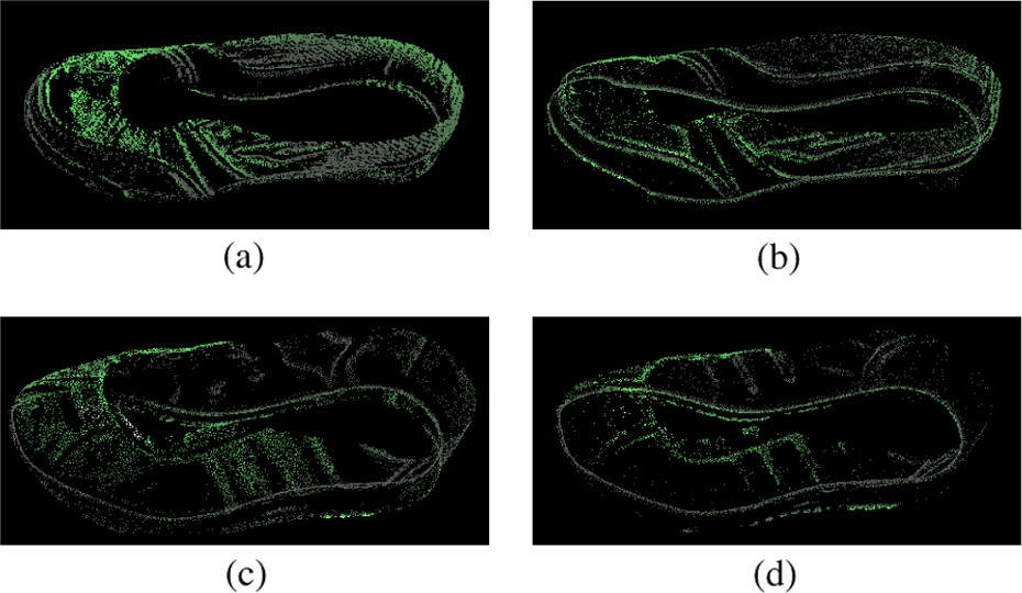
On the basis of referring to the SVD decomposition, our algorithm uses the PCA decomposition with weighted values to weight the data matrix M according to the distance to reference point, which can get high performance for exacting the nonsharp smooth feature like the shoe groove. In Figure 12, we compare the results obtained by SVD decomposition and the weighted PCA feature analysis.

Figure 12.

The experimental results of feature extraction: (a) result of SVD decomposition, (b) result of weighted PCA decomposition, (c) result of SVD decomposition, and (d) result of weighted PCA decomposition. PCA: principal component analysis.

From Figure 12(a) and (c), the result of SVD decomposition, we can see that the original algorithm cannot suppress noise; in addition to the shoe-groove line features, there are a lot of points even in the smooth regions. The improved algorithm of weighted PCA decomposition has a good retention for the shoe-groove line but suppresses the points in flat areas, see Figure 12(b) and (d).

When extracting the features, the characteristics of positive and negative mean curvature H are convex and concave. As the shoe groove is concave, the corresponding mean curvature is negative. The concave feature of the shoe groove is shown in Figure 13. The blue dashed-line is the shoe groove from which a segment profile in red is plotted, see Figure 13, right.

Figure 13.

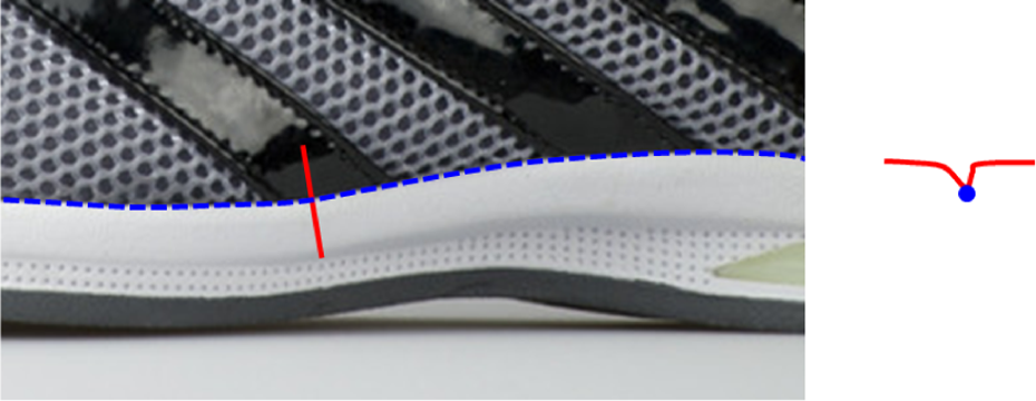
A groove example. The blue dashed line illustrates the sole feature. Right image shows an intersection of the shoe surface and the sole.

From differential geometry, the mean curvature has large absolute value in valley area, see the red denotation in Figure 14. But it is difficult to directly employ the mean curvature to extract the shoe groove as there are some concave features with the same curvature, see Figure 14. We find that the shoe groove is a closed curve; however, it is difficult to detect it in 3-D spaces. In this article, we use dimensionality reduction method from 3-D to 2-D to detect the closed shoe groove.

Figure 14.

Mean curvature maps of the scanned point cloud (mean curvature is rendered in Meshlab Ver1.3.3 (http://meshlab.sourceforge.net/)).

Feature extraction using dimensionality reduction

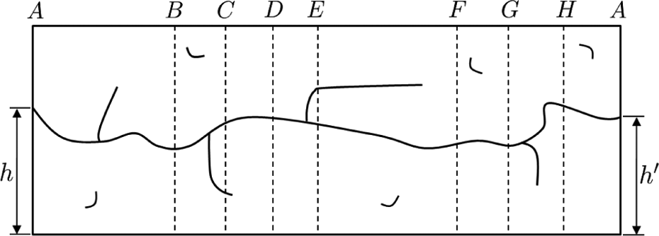
In order to facilitate the shoe-groove extracting, we project the feature points and incidental feature information of shoes to the two-dimensional images. First, we put the shoe inside a virtual cylinder shown in Figure 15 and divide the cylinder into eight sections, denoted by AB, BC, CD, DE, EF, FG, GH, and HA, which can be considered as 2-D images. Then, the data set in each section is projected onto the 2-D images, as shown in Figure 15. If we specify the Z axis positive outward direction perpendicular to the paper, the 3-D points on the same Z values locate on the same row in 2-D image (image scan lines represented as u). The projection is a subregional block projection. Influenced by the shoe size, the distance from AF to shoe toe and BE to shoe heel is roughly λ times of the shoe length (λ ranging from 0.1 to 0.2). The gray values in the projection images represent the values of feature information.

Figure 15.

Sketch map of feature information projection and the projected 2-D curvature map.

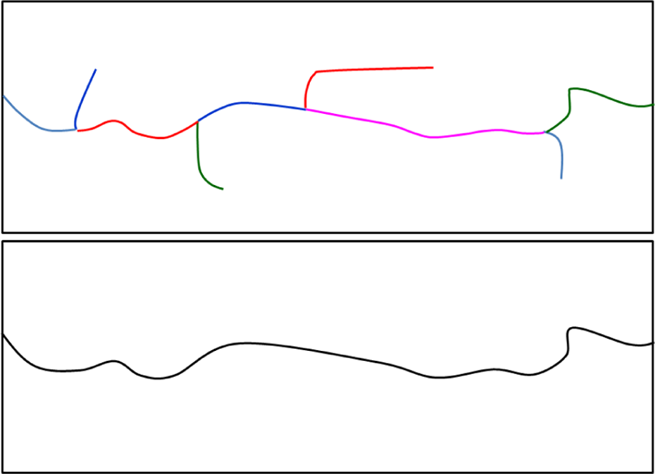
After combining these eight images into a single one, we can obtain a projected 2-D curvature map, as shown in the second row in Figure 15, from which we can find that the shoe groove is a continuous curve. We conduct the dimensionality reduction to simplify the shoe-groove extraction. The red pixels are extracted from the 2-D image, as shown in the bottom of Figure 15. We can search the shoe-groove feature from the extreme left to the extreme right. This feature line corresponds to the longest closed feature line in the three-dimensional model of the shoes, as shown in Figure 16.

Figure 16.

2-D image after projection.

Extracting the shoe groove in 2-D image

In the process of the projection, we set the pixel values of the projected point from 3-D space as the mean curvatures, from which a 2-D image can be constructed. Then, a 2-D closed feature curve is detected by the following steps:

Connect the points into line segments and set a threshold to filter out the short segments. We set the threshold equals to the width of combined 2-D image.

Determine the bifurcations along a curve. If there is a bifurcation, the curve is broken at this point from which another line segment is searched. Repeat steps (1) and (2) until all the points are traversed, see Figure 17.

Connect the line segments from left to right into a longest curve.

Back project the longest curve to 3-D space to get the coarse shoe-groove curve.

Figure 17.

Shoe-groove curve extraction in 2-D space.

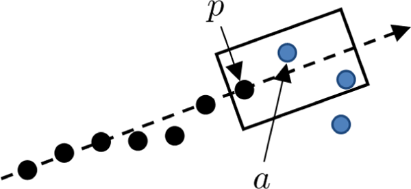
First, we traverse the 2-D image to find a nonzero point and its neighbors to a structure L vector < point >. To search for the next point, it is to find out the last K points in vector <point>, then fit these points to a straight line, and find a rectangular area along the straight line direction, and finally apply PCA method after weighted to these points in the rectangle according to feature size. Since the shoe groove within a small area is close to straight, if there is no diverging point, points in the rectangular area are proximately in a straight line, the eigenvalue of main component is relatively large, as illustrated in Figure 18. The black dots are the stored points in vector. To further extend the feature line, we can utilize the last few points K to fit a line to get the extension direction. Then, a rectangle is defined along this direction. The length and width ratio of the rectangle is 3:1. Point p is a last feature in vector, and in the rectangle contains two points, where point a is close to p. Therefore, a is stored in vector. Then, taking a is a start point to extend the line feature.

Figure 18.

Extension-based line segment extraction.

The bifurcations will occur during the process of line segment growth. At the bifurcation, at least one curve does not belong to the shoe-groove feature. If there is an intersection point, the line growth must be stopped. In the rectangle, we employ the PCA-based method to analyze the properties of the points. If the point set approximately lies on a line, the eigenvalue from PCA is larger. Then, we set a threshold ε = 0.7. If the eigenvalue is greater than ε, no bifurcation point is considered inside the rectangular region, then push the point into vector < point >, as shown in Figure 19. If the eigenvalue is less than ε, there exists bifurcation point inside the rectangular, then, stop pushing point into vector < point >, and a curve segment is formed. Next, take out the last few points from the right end of the rectangular area to create a new vector < point > structure; if there is no feature point in the right side of the rectangular area, we re-traverse the image and look for new feature points until all feature points are completely traversed to ensure that the feature points are all on the segment.

Figure 19.

Discrimination of diverging point in the shoe groove.

Through the aforementioned steps, we can get some line segments that are stored in vector < vector < point >>. Next, these line segments will be connected to a longest feature line that extends from left to right of the image. Since the vector < point > is in ascending order from left to right in the image, then if two line segments are both part of the shoe groove and connected segment to segment. If two segments belong to the shoe groove, the main directions of the two segments are approximately the same according to the characteristic of shoe groove. In other words, the inner product of these vectors is less than a small value, and then connects them to a new curve segment. Iterate the aforementioned procedure until the line is extended from the left to right of the image. The heights of shoe groove in the projected image are almost the same because the shoe groove is a closed curve, see Figure 16, for example, h ≈ h′, which can be used to verify the correctness of the result. Then, the detected line is exactly the projection of shoe groove in 2-D image. According to the correspondence of the 2-D and 3-D points, we can back project this 2-D curve to 3-D space. Finally, we can obtain the shoe groove in the 3-D space. But the shoe groove is very thick and disorder, so it requires further refinement and processing.

Thinning and extraction of the shoe groove

In order to compute the trackable sequential line segments, the rough edge must be thinned. Although the shoe groove is curve, we can use small line segments to approximate it. For a current point p, a line can be fitted in a neighborhood of point p. Then, the point p is projected to the fitted line and produced a new point p′. The space line equation is as follows

\frac{x - x_{0}}{m} = \frac{y - y_{0}}{n} = \frac{z}{1}

The parameters of m, n, x₀, and y₀ should be solved during fitting. As the shoe groove in 2-D is the longest closed line, we can determine the points order. Then, these points are projected into 3-D, and the topology will not be changed. So, we can extract λ points before and after point p, totally 2λ + 1, to fit the line. Equation (17) can be rearranged as follows

{\begin{array}{l} x = x_{0} + m z \\ y = y_{0} + n z \end{array}

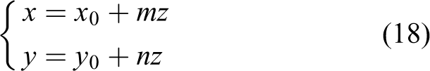
The matrix form of equation (18) is

[\begin{matrix} m & x_{0} \\ n & y_{0} \end{matrix}] [\begin{array}{l} z \\ 1 \end{array}] = [\begin{array}{l} x \\ y \end{array}]

Equation (19) of the i th point is expressed as

[\begin{matrix} m & x_{0} \\ n & y_{0} \end{matrix}] [\begin{array}{l} z_{i} \\ 1 \end{array}] = [\begin{array}{l} x_{i} \\ y_{i} \end{array}]

By using all of the points, we get

[\begin{matrix} m & x_{0} \\ n & y_{0} \end{matrix}] [\begin{array}{l} z_{1} \dots z_{n} \\ 1 \dots 1 \end{array}] = [\begin{array}{l} x_{1} \dots x_{n} \\ y_{1} \dots y_{n} \end{array}]

Equation (21) can be changed as

[\begin{matrix} m & x_{0} \\ n & y_{0} \end{matrix}] [\begin{array}{l} z_{1} \dots z_{n} \\ 1 \dots 1 \end{array}] [\begin{matrix} z_{1} & 1 \\ ⋮ & ⋮ \\ z_{n} & 1 \end{matrix}] = [\begin{array}{l} x_{1} \dots x_{n} \\ y_{1} \dots y_{n} \end{array}] [\begin{matrix} z_{1} & 1 \\ ⋮ & ⋮ \\ z_{n} & 1 \end{matrix}]

Equation (22) can be rewritten as

[\begin{matrix} m & x_{0} \\ n & y_{0} \end{matrix}] = [\begin{matrix} \sum x_{i} z_{i} \sum x_{i} \\ \sum y_{i} z_{i} \sum y_{i} \end{matrix}] {[\begin{matrix} \sum z_{i}^{2} \sum z_{i} \\ \sum z_{i} n \end{matrix}]}^{- 1}

Through equation (23), we can fit a line and project the point p to it. After all the other points are projected, this procedure is iterated. In practice, two iterations are enough to get the thinned shoe groove, as illustrated in Figure 20.

Figure 20.

Thinning result of shoe-groove point set.

Shoe groove obtained by the aforementioned steps is relatively messy; they should be fitted into a closed curve so that the robot can track and achieve automated polish, spray glue, and so on. This system takes running efficiency as a priority, utilizes projection of spatial curve to fit and refine the shoe groove, which selects to apply local spatial straight line fitting to each feature points in the shoe groove, and then projects the feature point to the straight line just fitted to generate a new shoe groove. Data processing is performed to all obtained feature points to obtain a smooth shoe groove. This method is faster than both non uniform rational B-spline (NURBS) curve fitting and B-spline curve fitting, well adapted to online computation. The trackable shoe groove and sequential segments are demonstrated in Figure 21. The right figure is a zoomed in portion of the feature line, which is represented as sequential segments and the corresponding normal vectors.

Figure 21.

The trackable shoe-groove and sequential segments.

Create new tracking curve for shoe upper

When a groove feature l_o with normal vector n_si is extracted from a sample shoe P_si, the feature line l_o is a sample from which the new trackable feature line can be created. In the shoe manufacturing process, a shoe without sole is scanned as point cloud P_sc, as shown in Figure 22, left, called current shoe upper. Then, the point clouds P_sc and P_si are aligned together with ICP method. After the alignment, a mesh model, P_aln, is reconstructed from point cloud _sc, and then along the normal vector n_si to compute the intersection point P_i with the surface model P_aln. All the intersection points constitute the closed tracking line l_sc. Finally, a robot manipulator can track the feature groove l_sc to accomplish automatic tracking, polishing, spraying glue, and other operations, see Figure 22, right.

Figure 22.

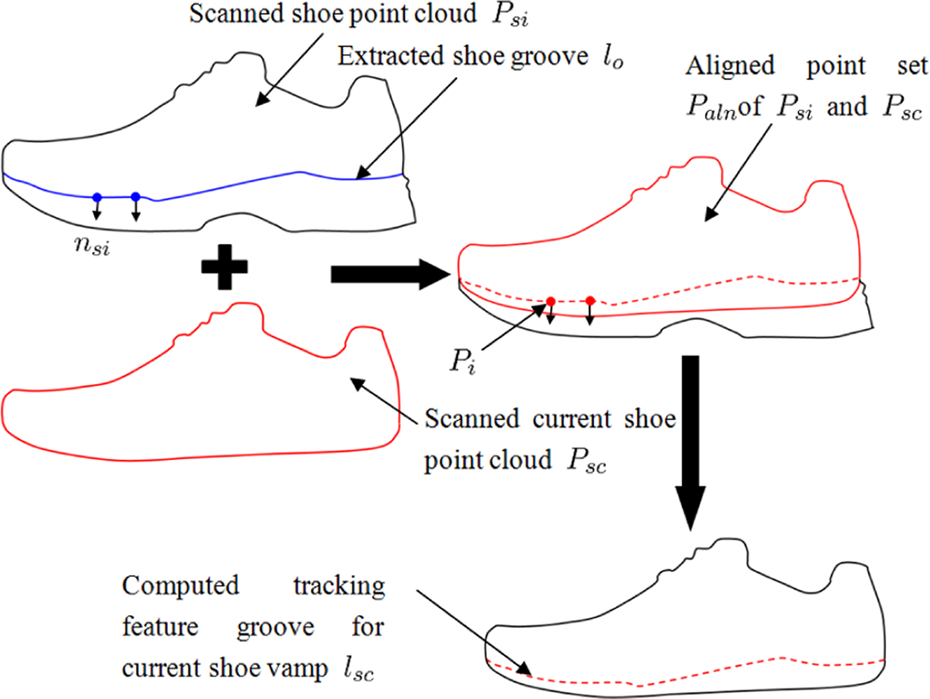
The procedures of new tracking groove creation.

Experiments

In this article, we propose a shoe-groove scanning and extraction system for robot tracking. We implement the proposed approach with VS2008, OpenCV, OpenGL, and a UR (https://www.universal-robots.com/) robot. The scanning device includes a Basler (www.baslerweb.com/) industrial camera, acA1600-20gm, with resolution 1626 × 1236, 20 fps, and GigE vision interface and a red line laser head. The experiment setup is demonstrated in Figure 23. The system is divided into some modules, such as image acquisition, laser plane calibration, hand-eye calibration, scanning, point cloud processing, feature line extraction, shoe-groove extraction, display, and so on. In this article, only some important modules are presented.

Figure 23.

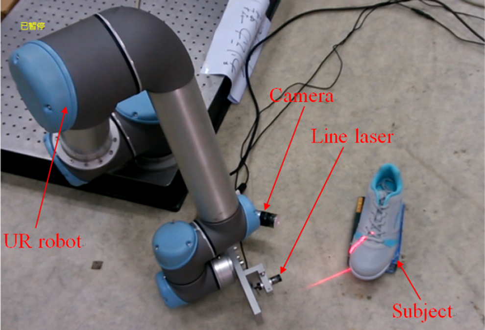
Hardware configuration of the experiment setup. The laser scanning device is mounted on the robot end effector.

We have conducted extensive evaluation of our proposed method. Figure 10(a), (c), and (e) give three subjects of scanning. Figures 24(a), 25(a), and 26(a) are the rendered 3-D point clouds with normal. Figures (b) to (e) in Figures 24 to 26 are the sequential results of processing, from feature extraction to thinned shoe groove. Figures (f) in Figures 24 to 26 are the final results of the shoe-groove extraction from which we can find that the main feature points can be remained. In order to verify the tracking effect, we utilize a 3-D visualization tool for ROS, rvis (https://github.com/ros-visualization/rviz) to simulate the tracking process. We establish a manipulator with 6-DOFs, and the sequential points in figures (f) of Figures 24 to 26 are input into an rvis simulation environment. Figure 27 demonstrates two poses of robot tracking in simulation environment. As it is a prototype system, the scanning and data processing speed are not fast enough to deploy it on a shoe making line. The scanning speed is about 2 min and the data processing is less than 3 s.

Figure 24.

Example I: Shoe-groove extraction procedures from scanned point cloud to sequential points. (a) Point cloud, (b) feature extraction, (c) denoising, (d) rough shoe groove, (e) thinned shoe groove, and (f) sequential points.

Figure 25.

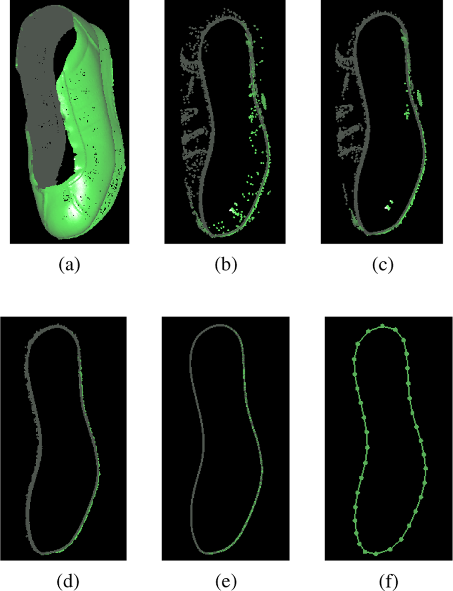
Example II: Shoe-groove extraction procedures from scanned point cloud to sequential points. (a) Point cloud, (b) feature extraction, (c) denoising, (d) rough shoe groove, (e) thinned shoe groove, and (f) sequential points.

Figure 26.

Example III: Shoe-groove extraction procedures from scanned point cloud to sequential points. (a) Point cloud, (b) feature extraction, (c) denoising, (d) rough shoe groove, (e) thinned shoe groove, and (f) sequential points.

Figure 27.

Shoe-groove tracking example based on a robot manipulator.

As there is not any benchmark of shoe model, we cannot evaluate the reconstruction accuracy quantitatively. In Figure 28, the top figure is an experimental subject, and there are many fine features on the surface; the bottom is the reconstructed surface model from which we can observe that the fine details, such as fabric texture, stitches, and so on, can be well recovered. In order to quantitatively compare the accuracy of our proposed system and the state-of-the-art technique, we utilize a commercial 3-D laser scanner, Creaform Handyscan, to reconstruct subject II and obtain a mesh model. Then, this mesh and the model created by our system are input into Geomagic studio 2010 and aligned these two meshes together. Next, we crop two meshes to get same overlap area to compute the discrepancy, as shown in the top figure in Figure 29. Finally, we can get the differences of these two models, illustrated in the bottom of Figure 29. The positive maximum distance is 0.22 mm and the negative maximum distance is −0.38 mm. The positive and negative average distances are 0.012 mm and −0.017 mm, respectively, as shown in Table 1. From these results, we can find that the reconstruction accuracy is comparable with the state-of-the-art method. Unlike the traditional 3-D scanner that needs stick markers on the surface to align the different patches, one advantage of our method is that the 3-D shoe model can be scanned and reconstructed automatically, no markers and no alignment. The hand-held Handy laser scanner costs over 10 min from scanning to data processing. Furthermore, in shoe manufacturing industry, the requirement of accuracy is not very high. Therefore, we conclude that the reconstruction accuracy is adequate enough to meet the 3-D reconstruction requirement in our system.

Figure 28.

3-D reconstruction accuracy comparison of the experimental subject and the reconstructed model.

Figure 29.

Quantitative analysis of reconstruction accuracy between the mesh created by our system and the mesh generated from Creaform Handyscan laser scanner.

Table 1.

Quantitative comparison of the reconstruction accuracy.

Maximum distance (mm)	Positive 0.22 Negative −0.38
Average distance (mm)	Positive 0.012 Negative −0.017
Standard deviation (mm)	0.0238
RMS estimate (mm)	0.0239

RMS: Root Mean Square.

In order to validate the effectiveness of the proposed algorithm, we compare the feature line extraction results with the Geomagic studio. The extracted feature lines are illustrated in Figure 30. The right figure in Figure 30 is a zoomed in portion of the shoe surface. From the figure, we can find that the method of Geomagic studio software can extract more feature lines, and there are bifurcations on the extracted lines. Figure 31 illustrates the results of subjects I and II. Comparing the results in Figures 24 to 26, 30, and 31, we can find that our proposed method can exactly detect the shoe-groove features. In Geomagic studio, we have to generate the surface mesh to extract the feature lines. But our method can directly extract the feature lines on point data set.

Figure 30.

Feature line extraction on shoe surface of subject III by using Geomagic studio.

Figure 31.

Feature line extraction on shoe surface of subjects I and II by using Geomagic studio.

One of the limitations of our method is that the black leather surface, the shoes without shoe-groove line, and the shiny surface cannot be scanned and reconstructed. In these cases, our method will fail to reconstruct the shoe-groove feature.

Conclusion

This article proposes a three-dimensional shoe-groove feature detection and tracking system to automatically accomplish the grinding and spraying by using a robot in shoe making industry, which can save lots of work force and improve the product quality. First, the hardware and software are designed, such as the scanning device, the camera calibration, laser plane calibration, and hand-eye calibration. In the 3-D feature analysis, we present a level-set-based total least-squares algorithm combined with the weighted PCA to improve the fitting precision and reliability. From the scanned point cloud, the Gaussian curvature and mean curvature are computed; the shoe groove becomes distinguishable as its concave property. Then, we project the point cloud from 3-D to 2-D. In 2-D space, the shoe-groove feature can be easily detected because it is a closed and longest curve on shoe surface. Next, the feature lines are thinned and sorted to acquire a sequential shoe groove. In the final step, a shoe vamp is scanned by the scanning device and the point cloud is obtained. After aligning the two data sets of shoes, the shoe groove of the current piece can be calculated. It can be tracked by a robot manipulator to finish some operations. Through this system, we can save labor force and cost. A limitation of our method is that the processing speed is not very fast to meet the real-time requirement. In the future, we can optimize the algorithm to improve the speed.

Footnotes

Declaration of conflicting interests

The author(s) declared no potential conflicts of interest with respect to the research, authorship, and/or publication of this article.

Funding

The author(s) received no financial support for the research, authorship, and/or publication of this article.

References

Galantuccia

Piperib

Lavecchiaa

. Semi-automatic low cost 3D laser scanning systems for reverse engineering. Procedia CIRP 2008; 28: 94–90.

Page

Koschan

Abidi

. Methodologies and techniques for reverse engineering – the potential for automation with 3-d laser scanners. In: Raja

Fernandes

(eds) Reverse engineering: an industrial perspective. Berlin: Springer Publishing House, 2008, pp. 11–32.

Blodow

Rusu

Marton

. Partial view modeling and validation in 3D laser scans for grasping. In: IEEE-RAS international conference on humanoid robots – humanoids, Paris, France, 7–10 December 2009, pp. 459–464. IEEE Press.

Guo

Zhu

. Large depth-of-view portable three-dimensional laser scanner and its segmental calibration for robot vision. Opt Lasers Eng 2007; 45(11): 1077–1087.

Harrison

Newman

. High quality 3D laser ranging under general vehicle motion. In: “High quality 3D laserranging under general vehicle motion” IEEE International Conference on, Robotics and Automation, Pasadena, California, USA, 19–23 May 2008, pp. 1–8. IEEE Press.

Fan

. On structured light vision sensor calibration in a robot based 3D laser scanning system. In: IEEE international conference on robotics and biomimetics (ROBIO), Guilin, China, 19–23 December 2009, pp. 1312–1316.

Bitelli

Dubbini

Zanutta

. Terrestrial laser scanning and digital photogrammetry techniques to monitor landslide bodies. In: International archives of the photogrammetry, remote sensing and spatial information sciences; In Proceedings of the 20th ISPRS congress, Geo-Imagery Bridging Continents, Istanbul, Turkey, 12–23 July 2004, Vol. XXXV, Part 5, pp. 246–251.

Elmqvist

Jungert

Lantz

. Terrain modelling and analysis using laser scanner data. Int Arch Photogramm Remote Sens 2001; 34(3): 219–226.

Yen

Akin

Lofton

. Using mobile laser scanning to produce digital terrain models of pavement surface, AHMCT Research Report: UCD-ARR-10-11-30-01, National Technical Information Service, Springefield, Virginia, November 30, 2010.

10.

Reutebuch

McGaughey

Andersen

H-E

. Accuracy of a high-resolution lidar terrain model under a conifer forest canopy. Can J Remote Sens 2003; 29(5): 527–535.

11.

Ingensand

Ryf

Schulz

. Performances and experiences in terrestrial scanning. In: Proceedings of the 6th conference on optical 3D measurement techniques (eds A

Grün

Kahmen

), Zurich, 22–25 September 2003, pp. 236–244. ETH Zurich.

12.

Dawson

Bertulli

Levy

. Application of 3D laser scanning to the preservation of fort conger, a historic polar research base on northern Ellesmere island, Arctic Can 2013; 66(22): 147–158.

13.

Huber

Akinci

Tang

. Using laser scanners for modeling and analysis in architecture, engineering, and construction. In: The 44th annual conference on information sciences and systems (CISS), Princeton, NJ, 17–19 March 2010, pp. 1–6.

14.

Isheil

Gonnet

J-P

Joannic

. Systematic error correction of a 3D laser scanning measurement device. Opt Lasers Eng 2011; 49(1): 16–24.

15.

Wang

A G

. A novel mechatronic design of a 3D laser scanning system. Int J Adv Mechatronic Syst 2010; 2(1/2): 124–131.

16.

Arias

Meneses

. A hand-held 3D laser scanning with global positioning system of subvoxel precision. JPCS 2011; 274(1): 1–7.

17.

Song

Feng

. A progressive point cloud simplification algorithm with preserved sharp edge data. Int J Adv Manuf Technol 2009; 45(5): 583–592.

18.

Endres

Hess

Engelhard

. An evaluation of the RGB-D SLAM system. In: IEEE international conference on robotics and automation (ICRA), St Paul, MN, USA, 14–18 May 2012, IEEE press.

19.

Shotton

Fitzgibbon

Blake

. Real-time human pose recognition in parts from a single depth image. Commuun ACM 2013; 56(1): 116–124.

20.

Henry

Krainin

Herbst

. RGB-D mapping: using Kinect-style depth cameras for dense 3D modeling of indoor environments. Int J Robot Res 2012; 31(5): 647–663.

21.

Robofoot project, http://www.robofoot.eu/ (accessed 12 August 2016).

22.

Tong

. A variational approach for detecting feature lines on meshes. J Comput Math 2016; 34(1): 87–112.

23.

Yoshizawa

Belyaev

Yokota

. Fast, robust, and faithful methods for detecting crest lines on meshes. Comput Aided Geom Des 2008; 25(8): 545–560.

24.

Ohtake

Belyaev

Seidel

H-P

. Ridge-valley lines on meshes via implicit surface fitting. ACM Trans Graph 2004; 23(3): 609–612.

25.

Strobl

Hirzinger

. Optimal hand-eye calibration. In: Proceedings of the IEEE/RSJ international conference on intelligent robots and systems (IROS 2006), Beijing, China, 9–15 October 2006, pp. 4647–4653.

26.

Shiu

Ahmad

. Calibration of wrist-mounted robotic sensors by solving homogeneous transform equations of the form AX = XB. IEEE Trans Robot Autom 1989; 5(1): 16–29.

27.

Hoppe

DeRose

Duchamp

. Surface reconstruction from unorganized points. ACM 1992; 26(2): 71–78.

28.

Chen