
Abstract
Linear quadratic regulator is a powerful technique for dealing with the control design of any linear and nonlinear system after linearization of the system around an operating point. For small systems, which have fewer state variables, the transformation of the performance index from scalar to matrix form can be straightforward. On the other hand, as the system becomes large with many state variables and controllers, appropriate design and notations should be defined to make it easy to automatically implement the technique for any large system without the need to redesign from scratch every time one requires a new system. The main aim of this article was to deal with this issue. This article shows how to automatically obtain the matrix form of the performance index matrices from the scalar version of the performance index. Control of a full-vehicle in cornering was taken as a case study in this article.
Keywords
Introduction
Linear quadratic regulator (LQR) problem is a useful and well-established method for solving the control forces of linear systems, and it has been proven to be stable and robust, provided the system is controllable. 1 A large part of the development of the LQR control method relies on the choices of the weighting factors of the performance index. Normally, the performance index is given in terms of the sum of the square of some state variables that need to be minimized. For the ease of mathematical manipulation, the performance index is usually rewritten in matrix form. In the case the performance index only contains a few state variables to be minimized, the transformation of the performance index from its scalar version to its matrix version is straightforward and does not require any effort. On the other hand, for some other systems with a more reliable mathematical model, the performance index might contain some other variables to minimize, which are not directly a state space variable, but are expressed in terms of a combination of state space variables. For example, in the case of vehicle attitude control, one may want to minimize the heave, pitch and/or roll acceleration, which is not defined as a system’s state, but it is expressed as a combination of state space variables. In this case, the transformation from the scalar form of the performance index to the matrix form needs some effort. The complexity can even increase depending on the type of system to be controlled.
One research area, where the LQR control strategy has been used extensively, is the control of a ground vehicle’s active suspension. The full-vehicle system usually consists of a seven degree of freedom model with only four control actuators, which makes the system uncontrollable. For this reason, many studies of the full-vehicle control have circumvented this by applying other techniques, such as filtered feedback control and input decoupling transformation, 2 sliding mode control, 3,4 or backstepping control. 5 The input decoupling transformation control strategy consists of inner control loops that reject road disturbances, outer control loops that stabilize heave, pitch and roll motions, and an input decoupling transformation that blends the inner and outer control loops.
Unlike the aforementioned decoupling transformation control strategy, which consists of an inner and outer control loop, the method used in this study treats the sprung and unsprung mass as a whole system, and the optimal control is applied to minimize the states included in the performance index. Although the solution of this technique depends heavily on the controllability of the system, the solution can still be obtained, even when the system is uncontrollable, depending on the choice of weighting factors. Since the performance index is normally given in the scalar form, whereas the LQR control technique is solved in matrix form, a systematic algorithm for the transformation of the performance index from scalar to matrix form is derived in this article to automatize this transformation for the performance index of any linear system. The remainder of this article is organized as follows: section “Problem formulation” presents the formulation of the problem, section “Relationship between the weighting factor matrices and the system matrices” describes the performance index transformation technique, section “Application example: full-vehicle attitude control in cornering” gives an example of full-vehicle attitude control, section “Simulation results” reports the simulation results, and section “Conclusion” provides some useful conclusions.
Problem formulation
The linearized form of any nonlinear system can normally be placed in the following linear equation

where x is the state vector, u is the control force, w is the external disturbance to the system,
where fi(x) represents a variable that is not defined as state variable, but is rather a combination of other states’ variables. For example, in the case of the attitude control of a full-vehicle, the suspension deflection is not defined as a state variable. fi(x) may represent the ith suspension deflection because the suspension deflection depends directly on the heaving, pitching, and rolling motion of the chassis.
Note that when the state space is suitably defined such that the performance index only contains the states variables, then fi(x) = 0.
The system’s matrices can be rewritten as
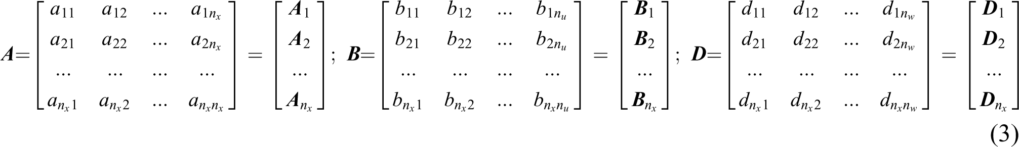
with

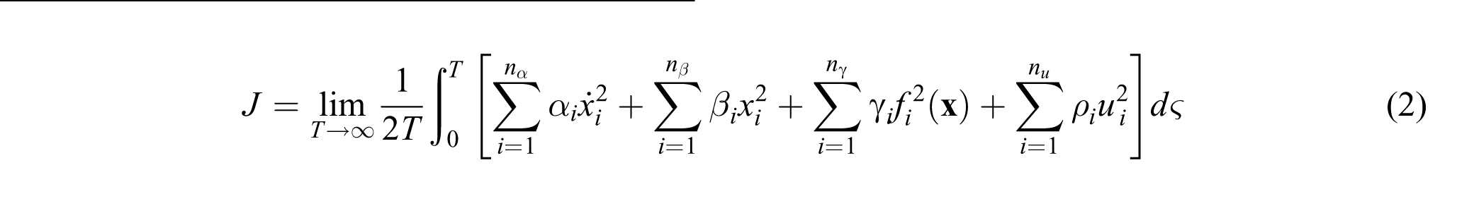
In order to solve the optimal control force, the performance index (2) should be transformed in the following form
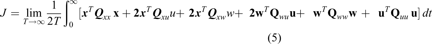
An algorithm was developed to solve the matrices
Relationship between the weighting factor matrices and the system matrices
The performance index (2) is comprised of four blocks, consisting of the following variables:
Contribution of the block
for the performance index matrices
From the state space equation (1), the derivative of a given state variable can be written as

The dimensions of the matrices and vector should be checked every time for consistency. Equation (6) is consistent because the dimensions of

Equation (7) can be developed step by step, or quickly using the following identity equation

Equation (7) can be expanded as

or

Note that because

The matrices in equation (10) can be expressed as

Therefore, to form each matrix in equation (5), the contribution of all the

Contribution of block
for performance index matrices
The contribution of this block to the performance index matrices is straightforward because there is no cross multiplication between the state variables and the control input or external disturbance. The contribution of this block is given as

with

Contribution of block
for performance index matrices
fi(

After squaring and expanding, the contribution of the term

Contribution of the block
for the performance index matrices
The term

Therefore, finally, the performance index matrices in equation (5) can be expressed as

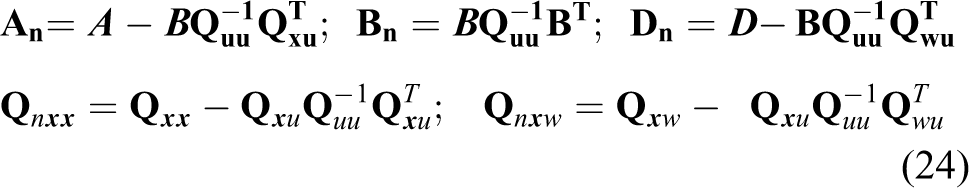
After deriving the performance index matrices, as shown in equation (19), the problem can now be solved easily because it is already well established that the control force vector that minimizes the object function (5) is given as

with

The matrix

The closed loop system is given by

The matrices are defined as
Application example: Full-vehicle attitude control in cornering
This example of a full-vehicle control is a good application because the system is not only an under-actuated control system (fewer control inputs than degrees of freedom) but also an uncontrollable system that requires more attention for the development of the optimal control forces.
Vehicle model
The full-vehicle model used in this article, as example, is given in Figure 1. The full-vehicle linear model consists of seven degrees of freedom: heaving, rolling and pitching motion for the vehicle chassis, and the remaining four degree of freedom for the wheel vertical displacements. For the dynamics equations of the car body see the study by Tchamna et al. 6
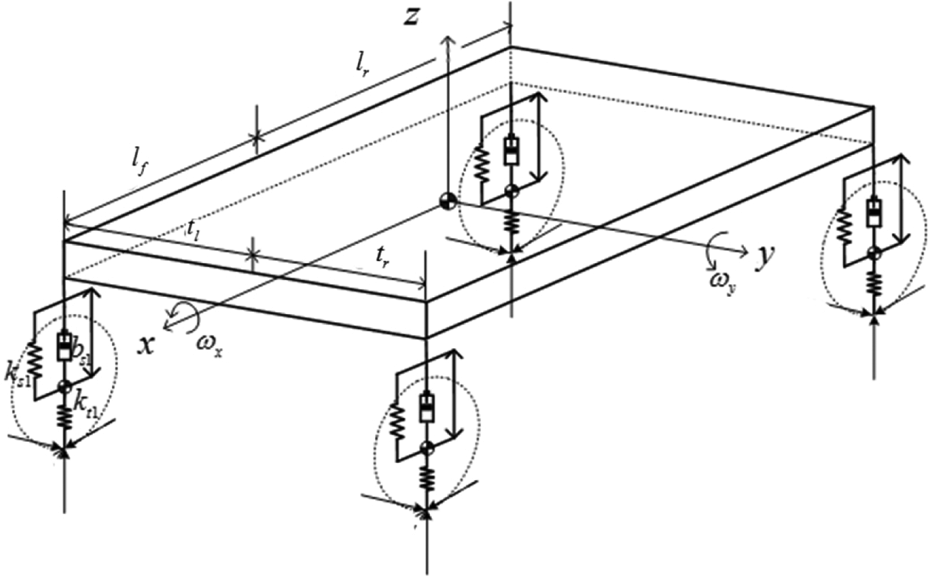
Full-vehicle linear model.
State space definitions
The state space variables of the full-vehicle should be defined based on the control design goal. One of the simplest ways of defining the state space variables of a system is to define it in terms of the body velocities and positions in addition to the wheel vertical velocities and positions, as follows
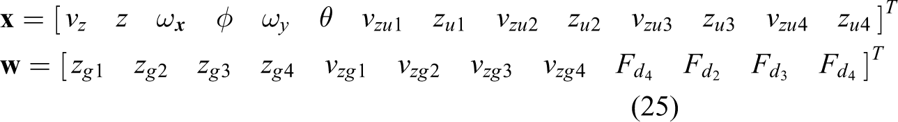
The system can be controlled using the state definitions given in equation (25). On the other hand, if the states are defined as in equation (25), the designer does not have direct control of the suspension deflections and tire deflections. To have direct control of the suspension rattle space, and tire deflection, another definition of the state variables can be given, as follows

The states defined in equation (26) are more appropriate compared to those in equation (25) because the states are defined in terms of the chassis velocities, unsprung mass velocities, suspension deflections, and tire deflections. Youn et al.
7
introduced the integral of the suspension deflections

A further examination of the definition of the states in equation (26) showed that although they can be used in the design of the active suspension control force, they only contain the velocity states of the chassis. To act directly on the car body position (the heave, pitch, and roll motion), those states need to be defined as a state variable. Therefore, another state variable can be defined by adding those variables in equation (26) as follows

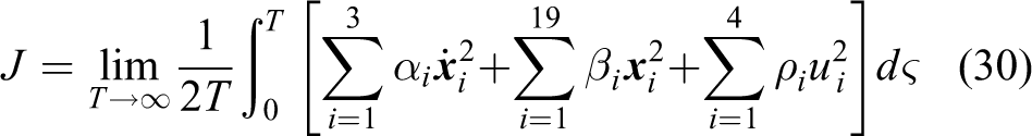
The state space variable defined in equations (26) to (28) will be used to design the control forces of the active suspension actuators. In the case, the systems states are defined as in equation (27) for example, the most general design of performance index can be expressed as

The motivation of choosing the index of the weighting factor, as above, is because the weighting index is needed to match the state variables index for easy implementation of the control algorithm, as will be shown later. Note that α i are the coefficients for the states derivative, β i the coefficients for the states, and ρ i for the control inputs, and all the indices of the coefficients should match those of the variables to keep the algorithm simple. The performance index (29) can be rewritten as
Likewise, the performance index for the state definition (28) can be written as follows

In the case the designer does not need to include a particular state in the performance index, he can just decide to turn the corresponding coefficient α i or β i to zero. For example, the generalized performance index for states (26) can be deduced from equation (31), by setting β16, β17, and β18 to zero. In the remainder of this article, systems 1, 2, and 3 denote the active suspension system designed using the states in equations (26), (27), and (28), respectively.
Simulation results
The simulation results of the full-vehicle travelling in cornering is displayed in this subsection. Figure 2 shows the distribution of the cornering forces acting on the vehicle when the steering wheel is applied to the vehicle. An external moment M
d

Cornering forces acting on the full-vehicle during cornering motion.
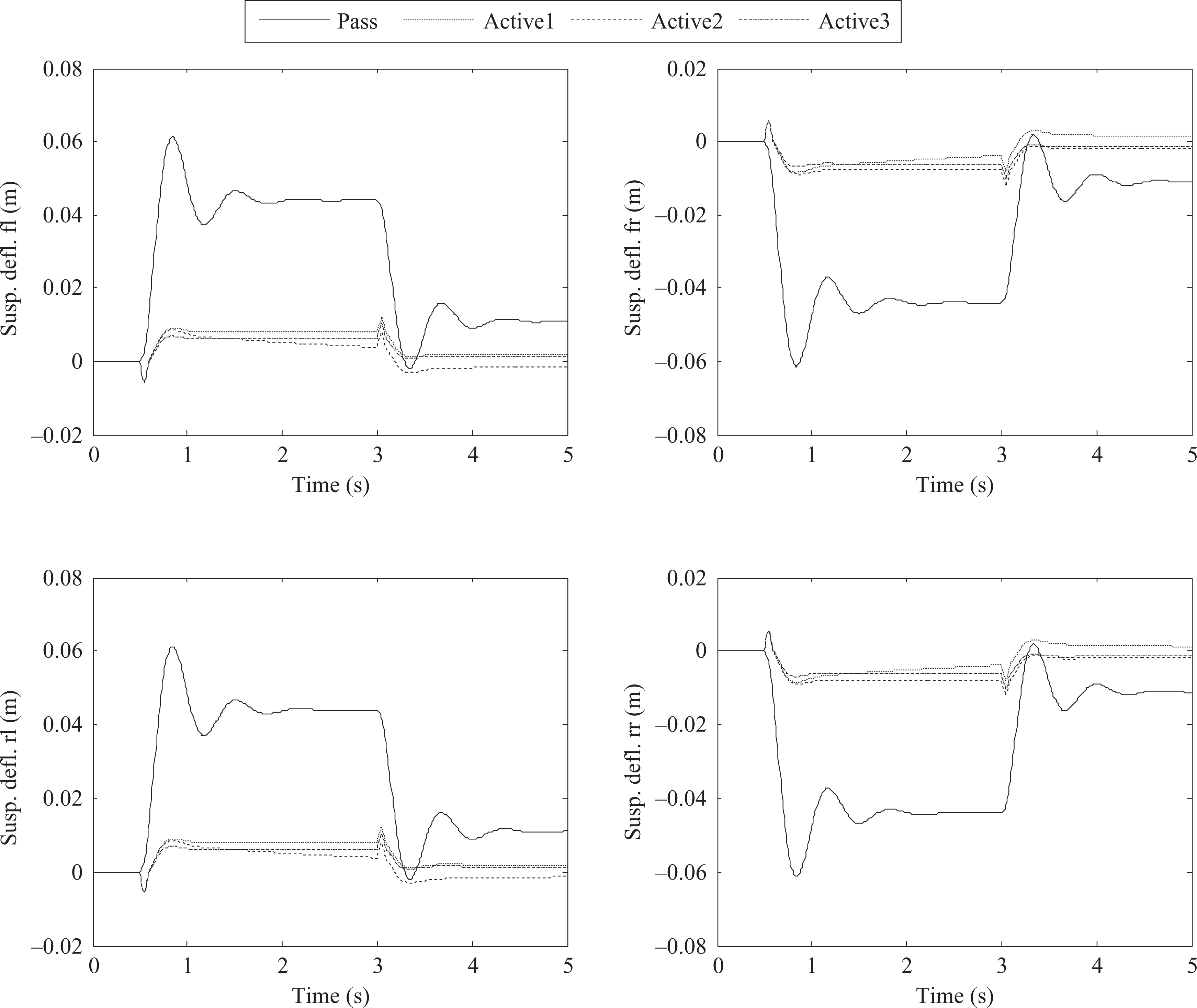
Suspension deflection of the full-vehicle during cornering motion.
Figure 4 shows the attitude motion of the vehicle (heave, roll and pitch motion). The same observations in Figure 3 were noted for this figure. Figure 5 is a magnification of the roll angle presented in Figure 4 because it is the main motion of interest during vehicle cornering. As can be seen, in the beginning (from 0 to about 1.7 s), although the system, active 3, which does not contain the integral of active suspension, performs better than the system, active 2, which contains the integral of suspension deflection, active 3 maintains a steady-state roll angle error, whereas active 2 tends to cancel that steady state roll angle error. The advantage of system active 3 over active 1 is emphasized more on this picture because a difference of approximately 0.5 degree can be observed between the two controlled systems.

Attitude of the full-vehicle during cornering motion.

Roll angle of the vehicle during cornering motion.
Conclusion
A systematic design of LQR optimal control performance index was presented using the appropriate notations that help generalize the transformation of the performance index from scalar to matrix form, for systems with large state variables. The method was then applied to attitude control of a full-vehicle in cornering. Suitable state variables were designed to solve the active suspension control force. This study can be useful for practical implementation of LQR for system with large state space variables.
Footnotes
Declaration of conflicting interests
The author(s) declared no potential conflicts of interest with respect to the research, authorship, and/or publication of this article.
Funding
The author(s) disclosed receipt of the following financial support for the research, authorship, and/or publication of this article: The work has been accomplished under the research projects no. APVV-15-0149, VEGA 1/0182/15, and KEGA 014STU-4/2015 financed by the Slovak Ministry of Education. This work was also supported by the 2014 Yeungnam University Research Grant.