Sage Journals: Discover world-class research

Abstract

This article studies the inverse kinematics problem of the variable geometry truss manipulator. The problem is cast as an optimization process which can be divided into two steps. Firstly, according to the information about the location of the end effector and fixed base, an optimal center curve and the corresponding distribution of the intermediate platforms along this center line are generated. This procedure is implemented by solving a non-convex optimization problem that has a quadratic objective function subject to quadratic constraints. Then, in accordance with the distribution of the intermediate platforms along the optimal center curve, all lengths of the actuators are calculated via the inverse kinematics of each variable geometry truss module. Hence, the approach that we present is an optimization procedure that attempts to generate the optimal intermediate platform distribution along the optimal central curve, while the performance index and kinematic constraints are satisfied. By using the Lagrangian duality theory, a closed-form optimal solution of the original optimization is given. The numerical simulation substantiates the effectiveness of the introduced approach.

Keywords

Variable geometry truss manipulator inverse kinematics Lagrangian dual optimization

Introduction

The variable geometry truss (VGT) manipulator is a candidate for a hyper-redundant mechanical system. It has a number of variable length members as its actuators and the topology of a statically determinate truss structure. Since it has the advantage of being comparatively lightweight and of high rigidity, it is expected to be used for future space and undersea exploration and inspection (see Miura et al.¹).

In the early 1980s, the concept of a VGT was derived from that of adaptive structures (see Miura and Furuya²). Since then, much attention has been paid to studies on the dynamic analysis and control (see Lee and Sanderson³), workspace analysis (see Badescu and Mavroidis^4,5) and conceptual and practical structures of VGT manipulators (see Hanahara and Tada⁶ and Rost et al.⁷). The inverse kinematics of the VGT manipulator have an infinite number of solutions. That is, for a given position of the end effector, inducing a self-motion of the manipulator without changing the position of the end effector is possible. Consequently, an effective selection criterion is required.

Much effort has been devoted to redundancy resolution by using “backbone curve” or “reference spline” to capture the macroscopic geometric features of the VGT manipulator. Chirikjian and Burdick^8,9 developed methods for determining an optimal curve describing the configuration of the VGT manipulator. In their proposed modal hyper-redundancy resolution approach, the backbone curve shape function was constrained to a modal form while the functions were limited only to a set of modes. Moreover, no direct means of satisfying constraints related to the end effector pose was provided in the latter approach⁹ and a careful selection of modes was required. What is more, the complexity of the method makes it very expensive for solving the inverse kinematics of a hyper-redundant manipulator in 3D operation space in real time. Fahimi et al.¹⁰ expanded the modal method and applied it to resolve the inverse kinematics for spatial hyper-redundant robots by using a new form function to change the mode. Nevertheless, this approach seems to be restricted to the situation in which the hyper-redundant manipulator is of a serial chain. Zanganeh and Angeles¹¹ proposed a spline-based solution approach, for given optimality criteria, in which they resolved the redundancy by seeking the optimal shape of the backbone curve. However, the authors supposed a fixed distribution of the intermediate platforms along any candidate curve.

On the other hand, studies of VGT manipulators in recent years have concentrated on two main structures: manipulators powered by binary actuators with two stable states^12,13 and those whose actuator is continuous but not mounted on the mobile platform.^14–16 Atilla Bayram and M. Kemal Ogoren^12,13 investigated the conceptual design of a VGT manipulator with the first structure together with forward kinematics and position control through inverse kinematics of a spatial binary hyper-redundant manipulator in. For the second type of VGT manipulator, Nobuyuki Iwatsuki et al.¹⁴ described the kinematic analysis and presented a motion-control technique for the hyper-redundant robot. Julien Mintenbeck and Ramon Estana¹⁵ researched the design, modeling and control of a hyper-redundant 3-RPS parallel mechanism. Abdelhakim Chibani et al.¹⁶ proposed a deterministic optimization scheme to generate an optimal kinematic configuration for spatial hyper-redundant manipulators with multiple rigid parallel modules. However, works focusing on octahedral VGT robot manipulators are scarce. R. Aviles et al.¹⁷ developed two procedures to calculate the optimal damper distributions in VGTs in and then presented a new approach to solving the inverse dynamics of VGTs with elastic elements.¹⁸ Sven Rost et al.¹⁹ introduced the design and hydraulic actuation for VGT manipulators with octahedral modules having three degrees-of-freedom. Nevertheless, none of this research optimizes the inverse kinematics of the octahedral VGT manipulator since the later admits an infinite number of solutions.

The complexity of the structure of octahedral VGT manipulators makes its practical application face numerous challenges in the modeling and control. In this article, we are concerned with a fundamental problem: that is, how to generate an optimal kinematic configuration of the manipulator for a given operating configuration. By reducing the constraints of the physical structure of the VGT manipulator, we improve the inverse kinematics optimization model proposed by Yang et al.²⁰ and thus the positioning error gets reduced. As shown in Figure 1, for a prescribed task configuration of the end effector, there exist an infinite number of solutions that enable the VGT manipulator to achieve the desired goal. The difference between any two of these solutions lies in two aspects: the shape of the center line representing the entire manipulator posture and the distribution of the intermediate platforms along this center line. With this observation, we put forward an optimization process (see Figure 2) that enables us to produce an optimal kinematic configuration of the manipulator for a specified target location.

Figure 1.

variable geometry truss configurations specified by backbone curve.

Figure 2.

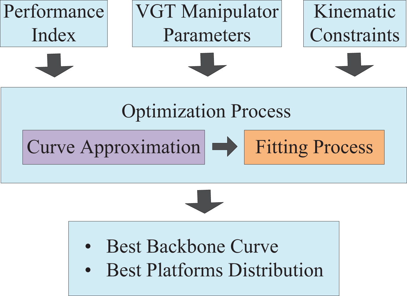
Optimization process of inverse kinematics.

The optimization process can be divided into two steps: curve approximation and the fitting process. In the stage of curve approximation, an optimal center curve and the distribution of the intermediate platforms along this center line are generated according to the information about the location of the end effector and fixed base. This process is implemented by solving a non-convex optimization problem that has a quadratic objective function subject to quadratic constraints. Then, in the fitting process stage, in accordance with the distribution of the intermediate platforms along the optimal center curve, all lengths of the actuators are calculated by using the inverse kinematics of each VGT module. Hence, the approach we present is an optimization procedure attempting to generate the optimal intermediate platform distribution along the optimal central curve, while the performance index and kinematic constraints are satisfied.

The remaining sections of this article are organized as follows. In the second section, we introduce the kinematics of the VGT manipulator. After that, in the third section, the inverse kinematics optimizing process for the VGT manipulators with n modules is formulated as a non-convex quadratic optimization problem. We solve the inverse kinematics optimization problem using a method based on the Lagrangian dual, and then the main conclusions and simulation results are given in the third and fourth sections, respectively. The final conclusions are given in the fifth section.

Kinematic analysis of the VGT manipulator

In this section, the kinematics of the VGT manipulator are analyzed on the basis of certain geometric structure constraints. We will introduce it from the following three parts: overall description, inverse kinematic modeling and backbone curve modeling of the VGT manipulator.

The VGT manipulator that we considered consisted of n identical parallel modules. Each module has three degrees of freedom. Each mobile platform is connected to the base platform of the module below and the associated platforms are assumed to be coincident (see Figure 3). Hence, the VGT manipulator has 3n degrees of freedom. In order to guarantee that the manipulator completes the desired task, we need to handle this large number of degrees of freedom judiciously. The first thing is to establish the relationship between the location parameters of the intermediate platforms and those of the end effector.

Figure 3.

Universal structure of the variable geometry truss manipulator.

Inverse kinematic modeling

The macroscopic kinematics of the VGT manipulator can be obtained according to the homogeneous transformation matrix as

T_{n}^{0} = T_{1}^{0} T_{2}^{1} \dots T_{n - 1}^{n - 2} T_{n}^{n - 1}

where $T_{i}^{i - 1}$ represents the homogeneous transformation matrix from the top platform to the base plane of the i th module of the VGT manipulator. Let the controlled actuator lengths be denoted by $L^{i}$ . Then the homogeneous transformation matrix can be deduced based on the relative movement of the two platforms $i - 1$ and i. If the vector of the posture of platform i versus platform $i - 1$ is denoted by $P_{i}^{i - 1}$ , then the microscopic inverse kinematics of the ith module of the VGT manipulator can be established by the relationship

L^{i} = f^{- 1} (P_{i}^{i - 1}), i = 1, 2, \dots, n

where $L^{i} = [L_{1}, L_{2}, L_{3}]_{i}^{T}$ is the column vector consisting of actuator lengths of the ith VGT module and f is the nonlinear mapping function representing the posture of the end effector with regard to the actuator lengths. When f is reversible, equation (1) is obtained. The analysis of the forward kinematics of a VGT module shows that the inverse model admits a unique solution.

Hence, for a desired end effector posture, it is necessary to determine the posture of all intermediate platforms at a macroscopic level, and then the length of each actuator can be worked out via the inverse kinematics of each VGT module. Nevertheless, due to the high redundancy of the VGT manipulator, this operation allows an infinite number of solutions. So establishing an optimization process to determine proper intermediate platform distribution and then calculating the length of each actuator will be of great help in solving this complicated problem. In Section 3, we will make a detailed introduction of the formulation of the inverse kinematics optimizing process and our proposed solution scheme.

Backbone curve modeling

The backbone curve is a piecewise curve that is usually used to describe the macroscopic kinematic characteristics of a hyper-redundant manipulator. In the method proposed by Chirikjian,²¹ a continuous backbone curve is used to assist solving inverse kinematics of binary manipulators. In the first phase, the inverse kinematics problem of the manipulator is solved to seek an idealized backbone curve to approximate the middle line of the manipulator. Then in the second phase, a fitting process is accomplished between the sought backbone curve and the joint variables. Inspired by this idea, in this article, we also adopt a method based on the backbone curve. However, the difference is that we directly define the curve as being composed of line segments connecting the two adjacent free control points as the backbone curve.

As shown in Figure 4, points $P_{S}$ and $P_{G}$ are the centers of the fixed platform at the bottom and the moving platform at the end, respectively. Points $P_{i} (i = 1, 2, \dots, n - 1)$ are $n - 1$ free control points that constitute the backbone curve. They can be determined according to the reachable working space of the overall manipulator structure and each VGT module as well as the distribution of obstacles. Therefore, we need to predefine a total of $n - 1$ control points to be connected in a preset order.

Figure 4.

Backbone curve and its coordinate systems.

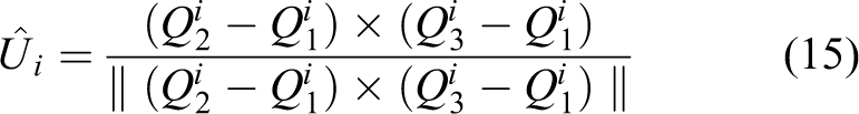
In order to describe the microscopic properties of the VGT manipulator, a reference coordinate system $P_{i} X_{i} Y_{i} Z_{i}$ is established using each free control point $P_{i}$ of the backbone curve as the origin. The $X_{i}$ axis is perpendicular to the attached platform and the $Z_{i}$ axis aligns with an edge of the triangle platform (see Figure 4).

Since the inverse kinematics solution of each VGT module is unique, as long as the free control point sequence is determined, the length of each actuator can be calculated directly. That is, once the homogeneous transformation matrix $T_{i}^{i - 1}$ is determinate, it is very straightforward to establish the length of each actuator of the ith VGT module. The inverse kinematics of a VGT module will be introduced in detailed in the following section.

In short, given an expected operating configuration of the end effector, a procedure for establishing an inverse kinematics model of the whole VGT manipulator and then solving for the corresponding length of each actuator could be described as follows.

Step 1. Generate the backbone curve constituted by starting point, terminal point and free control points, in accordance with the desired operating configuration of the end effector and distribution of obstacles.

Step 2. Fit the macro geometrical characteristics of the VGT manipulator to the generated backbone curve and calculate the n homogeneous transformation matrix $T_{i}^{i - 1}$ .

Step 3. Compute the length of the actuators of each VGT module $L^{i}$ .

Formulation of the optimizing process

As stated above, our approach is designed to intelligently process the basic problem of a VGT manipulator connected by multiple modules. Indeed, for an expected operating configuration of the end effector, there are an infinite number of solutions that the manipulator can make to reach it. These solutions are different from each other in accordance with the form of the backbone curve and the intermediate platform distribution along the backbone curve. Thus, for a prescribed performance indicator, we used an optimization procedure to evaluate the score of the backbone curves for a minimization.

Boundary conditions and physical limitations

The backbone curve fitting at the base and top platforms must satisfy the boundary conditions

P_{0} = P_{S}, P_{n} = P_{G}

where $P_{S}$ represents the location of the fixed platform at the bottom and $P_{G}$ is the posture of the moving platform on the top.

Furthermore, constraints describing the scope of each actuator length can be expressed as

L_{min} \leq L_{j}^{i} \leq L_{max}, i = 1, 2, \dots, n, j = 1, 2, 3

Obstacle avoidance

If there are obstacles in the workspace, the inverse kinematics consists of generating an optimal configuration that allows the manipulator to avoid the obstacles and achieve the specified target. In order to avoid obstacles, we append a series of auxiliary constraints to the optimization process to ensure that the robot does not collide with the obstacles. These constraints for obstacle avoidance should cover not only the structures of the manipulator and obstacles but also the positional relationship between them. Suppose we use a series of simple geometrical forms (such as cuboids, spheres or ellipsoids) to compute the minimum safety distance between the manipulator and obstacles around it. When spheres are chosen as the minimal bounding volumes of obstacles and the radius is taken for that placed on the manipulator(see Figure 5), the constraints can be represented in the general form

∥ P_{i} O_{j} ∥^{2} \geq {(L_{j} + L)}^{2}, i = 1, 2, \dots, n, j = 1, 2, \dots, m

where

P_{i}

is the ith free control point on the backbone curve,

O_{j}

is the position vector of the center of gravity of the j th obstacle with its radius

L_{j}

, L is the radius of the circumscribed circle of the middle platform, and m and n are, respectively, the number of obstacles and VGT modules.

Figure 5.

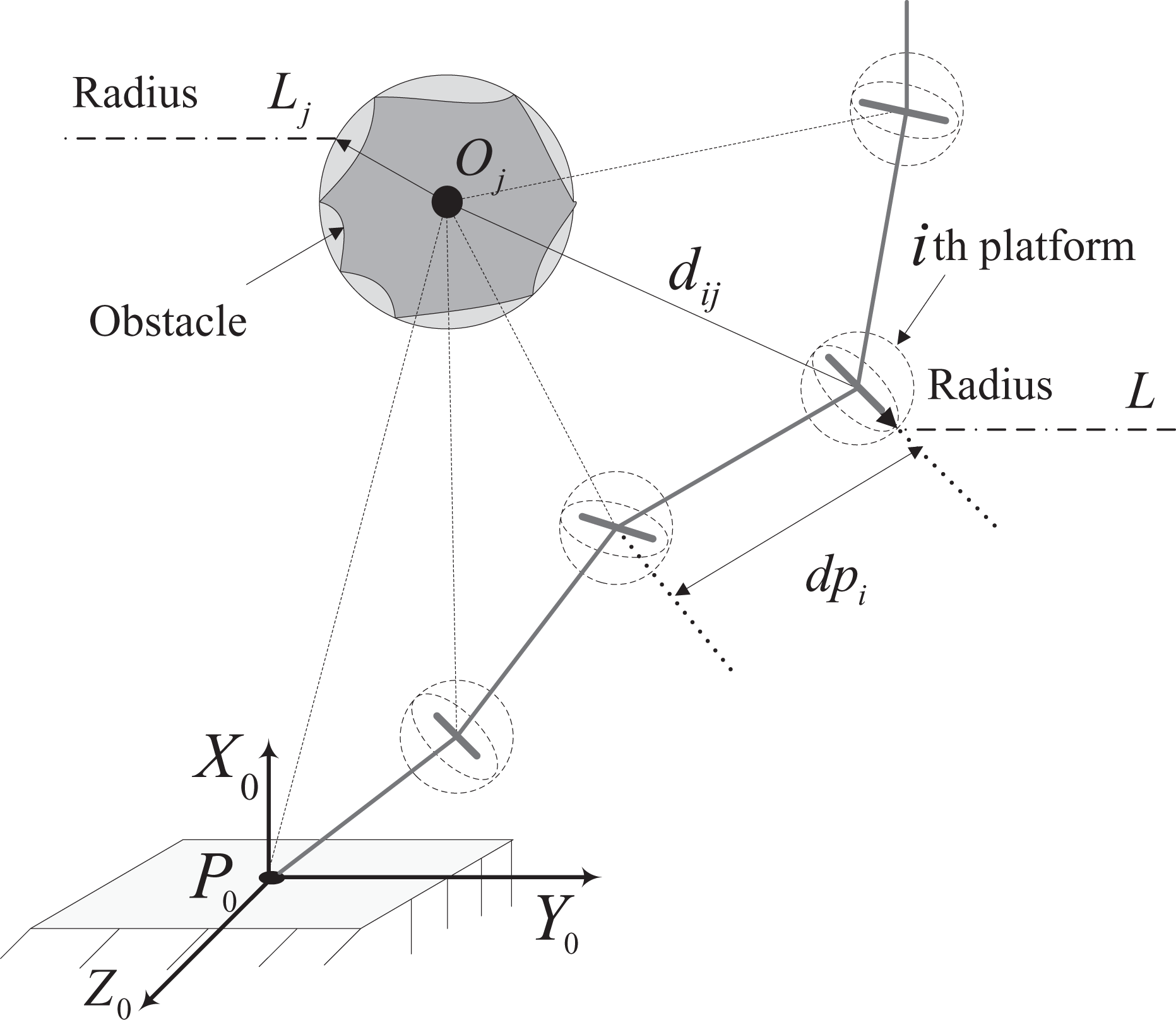
Details for obstacle avoidance.

Problem statement and solution

For simplicity, we represent the length of the ith line segment (whose starting point and end point are free control points $P_{i - 1}$ and $P_{i}$ , respectively) of the backbone curve by the variable $d p_{i}$ . Assume that $P_{t}$ represents the desired terminal position of the VGT manipulator. According to the variables defined above, the inverse kinematics optimization problem can be described as follows.

The distance between $P_{t}$ and $P_{n}$ needs to be minimized.

The length of each line segment $d p_{i}$ is in a specific range and is expected to be minimized.

The VGT manipulator can avoid collisions with obstacles. Suppose the j th obstacle is a sphere with the center $O_{j}$ and the radius $L_{j}$ .

Then the inverse kinematics problem can be described as

\begin{array}{l} min_{P} & ∥ P_{n} P_{t} ∥^{2} + \sum_{i = 1}^{n} k_{i} d p_{i}^{2} \\ subject to & d p_{min}^{2} \leq d p_{i}^{2} \leq d p_{max}^{2} \\ d_{i j}^{2} = ∥ P_{i} O_{j} ∥^{2} & \geq {(L_{j} + L)}^{2}, i = 1, 2, \dots, n, j = 1, 2, \dots, m \end{array}

where

d p_{i}^{2} = ∥ P_{i} P_{i - 1} ∥^{2} (i = 1, 2, \dots, n)

is the square of the length of the ith line segment of the backbone curve,

d p_{min}

and

d p_{max}

are, respectively, the known minimum and maximum lengths of

d p_{i}

k_{i}

is the weight coefficient of each line segment and

P^{T} = [(P_{1})^{T}, (P_{2})^{T}, \dots, (P_{n})^{T}]

is the output vector.

According to the physical meaning of each parameter in the model above, we will simplify the optimization problem.

In order to describe the optimization variables more simply and intuitively, we define matrices $A_{i} \in R^{3 \times 3 n}$ and

A_{i} = {\begin{matrix} \begin{array}{l} [ & O, O, \dots, I, \dots, O] i = 1, 2, \dots, n \\ O^{3 \times 3 n} i = 0 \end{array} \end{matrix}

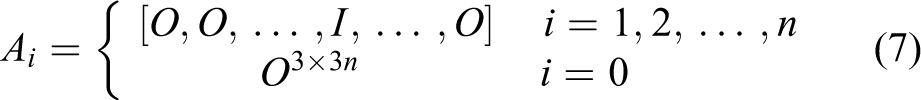
where O and I are a three-by-three order zero and the identity matrix, respectively. Then $P_{i} = A_{i} P$ and the square of the distance between $P_{n}$ and $P_{t}$ is

∥ P_{n} P_{t} ∥^{2} = P^{T} A_{n}^{T} A_{n} P - 2 P_{t}^{T} A_{n} P + P_{t}^{T} P_{t}

The square of the length of every rod is

d p_{i}^{2} = ∥ P_{i} P_{i - 1} ∥^{2} = P^{T} {(A_{i} - A_{i - 1})}^{T} (A_{i} - A_{i - 1}) P

The square of the length between $P_{i}$ and $O_{j}$ is

∥ P_{i} O_{j} ∥^{2} = P^{T} A_{i}^{T} A_{i} P - 2 O_{j}^{T} A_{i} P + O_{j}^{T} O_{j}

The minimization problem given in equation (6) finally becomes

\begin{array}{l} min_{P} & P_{t}^{T} P_{t} - 2 P_{t}^{T} A_{n} P + P^{T} [A_{n}^{T} A_{n} + \sum_{i = 1}^{n} k_{i} {(A_{i} - A_{i - 1})}^{T} (A_{i} - A_{i - 1})] P \\ s . t . d p_{min}^{2} \leq P^{T} {(A_{i} - A_{i - 1})}^{T} (A_{i} - A_{i - 1}) P \leq d p_{max}^{2} \\ P^{T} A_{i}^{T} A_{i} P - 2 O_{j}^{T} A_{i} P + O_{j}^{T} O_{j} \geq {(L_{j} + L)}^{2} i = 1, 2, \dots, n, j = 1, 2, \dots, m \end{array}

Obviously, the objective and constraint functions of the minimization problem are all quadratic, so they can be converted to linear matrix inequality(LMI) forms. Using Lagrange duality, the problem given in equation (11) can be solved by a convex optimization over LMIs as follows, and this will be demonstrated exhaustively in the appendix

\begin{array}{l} min & ρ \\ subject to & [\begin{matrix} K & M^{T} \\ M & ρ + 4 F \end{matrix}] \geq 0 \\ λ \geq 0, u \geq 0, v \geq 0 \end{array}

Numerical simulations

In this section, we put forward a simulation study on an octahedral VGT manipulator. This manipulator is composed of n spatial modules in the form of serial concatenation. Next, we will introduce the kinematics of a single VGT module of the mechanical arm, and then the corresponding simulation results are given.

Kinematics of single VGT module

The kinematic model for the VGT module is shown in Figure 6(a). $L_{1}, L_{2}$ and $L_{3}$ are three independently controlled linear actuators. By changing the length of the three actuators, the top platform can be moved with respect to the bottom platform. Referring to Figure 6(a), a fixed coordinate frame $P_{i - 1}^{r} X_{i - 1} Y_{i - 1} Z_{i - 1}$ is rigidly attached to the fixed base, with the origin at the center of the bottom. The $X_{i - 1}$ axis coincides with the normal to the base plane and the $Z_{i - 1}$ axis parallel to an edge of the base triangle. A moving coordinate system $P_{i}^{r} X_{i} Y_{i} Z_{i}$ is attached to the top moving face so that its origin is at the center of the top platform. The $X_{i}$ axis is perpendicular to the top plane and the $Z_{i}$ axis aligns with an edge of the top triangle. Let $θ_{1}, θ_{2}, θ_{3}$ denote the dihedral angles between planes $B_{1} B_{2} Q_{1}, B_{2} B_{3} Q_{2}, B_{1} B_{3} Q_{3}$ and plane $B_{1} B_{2} B_{3}$ , respectively, as shown in Figure 6(b). The meaning of all the other parameters in Figure 6(a) and Figure 6(b) are listed in Table 1.

Figure 6.

(a) Kinematic model for the variable geometry truss module; (b) parameters for the lower variable geometry truss half; (c) virtual extensible kinematic diagram.

Table 1.

Meaning of the variable geometry truss (VGT) parameters.

VGT parameters	Meanings of the parameters
L, $L_{0}$	Cross longeron and fixed batten length
$Q_{j}^{i} : Q_{1}^{i} Q_{2}^{i} Q_{3}^{i}$	Lower actuation plane nodes of the ith module
$L_{j}^{i} : L_{1}^{i} L_{2}^{i} L_{3}^{i}$	Lengths of the actuators for the ith VGT module
${\hat{n}}_{i}$	Unit normal for the ith module in the relative coordinate system
$O_{i} : O_{1} O_{2} O_{3}$	Steward platform revolute locations
r, S	Gimbal extension parameter, mid-plane joint offset
$P_{i}$ , $P_{i}^{r}$	Midpoint of the ith module in the base and relative coordinate system
$T_{P B}^{i}$	Transformation matrix
${\hat{U}}_{i}$	Mid-plane normal of the ith module
$θ_{i} : θ_{1} θ_{2} θ_{3}$	Cross longeron face angles

According to the coordinate frame established above, the coordinates of fixed points $O_{i}$ in frame $P_{i - 1}^{r} X_{i - 1} Y_{i - 1} Z_{i - 1}$ are described as $O_{1} {(0, - \frac{L_{0}}{2 \sqrt{3}},0)}^{T}$ , $O_{2} {(0, \frac{L_{0}}{4 \sqrt{3}}, - \frac{L_{0}}{4})}^{T}$ , $O_{3} {(0, \frac{L_{0}}{4 \sqrt{3}}, \frac{L_{0}}{4})}^{T}$ . Because the three cross longeron planes are identical, the length of $O_{i} Q_{i}$ equals $N = \sqrt{L^{2} - L_{0}^{2} / 4},$ and the unit vector directions $q_{i}$ pointing along $O_{i} Q_{i}$ are expressed as $q_{i} = (s i n θ_{i}, - c o s θ_{i} c o s φ_{i}, - c o s θ_{i} s i n φ_{i})^{T}$ , where $φ_{1} {= 180}^{o}, φ_{2} {= 300}^{o}, φ_{3} {= 60}^{o}$ . Then the position vectors of movable points $Q_{i}$ in the fixed coordinate frame $P_{i - 1}^{r} X_{i - 1} Y_{i - 1} Z_{i - 1}$ can be calculated according to the formula $Q_{i} = O_{i} + N q_{i}$ . Letting $E = \sqrt{12 L^{2} - 3 L_{0}^{2}} / L_{0}$ , $F = 4 L^{2} - L_{0}^{2}$ , $c θ = cos θ$ and $s θ = sin θ$ , the three scalar constraint equations of the reverse displacement analysis problem for an octahedral VGT manipulator can be written as

\begin{array}{l} c θ_{1} + c θ_{2} - E c θ_{1} c θ_{2} + 2 E s θ_{1} s θ_{2} - E / F (8 L^{2} - L_{0}^{2} - 4 L_{1}^{2}) = 0 \\ c θ_{2} + c θ_{3} - E c θ_{2} c θ_{3} + 2 E s θ_{2} s θ_{3} - E / F (8 L^{2} - L_{0}^{2} - 4 L_{2}^{2}) = 0 \\ c θ_{1} + c θ_{3} - E c θ_{1} c θ_{3} + 2 E s θ_{1} s θ_{3} - E / F (8 L^{2} - L_{0}^{2} - 4 L_{3}^{2}) = 0 \end{array}

When the symmetry of the model is taken into account, there are eight solutions for $θ_{i}$ in equation (13), while, in the actual situation, only one solution can be worked out. According to the geometric relationship of the VGT model, the location of the center of the top platform $P_{i}^{r}$ can be calculated by the following two equations from Boyd and Vandenberghe²²

P_{i}^{r} = (2 Q_{1}^{i} \cdot {\hat{U}}_{i} + S) {\hat{U}}_{i}

{\hat{U}}_{i} = \frac{(Q_{2}^{i} - Q_{1}^{i}) \times (Q_{3}^{i} - Q_{1}^{i})}{∥ (Q_{2}^{i} - Q_{1}^{i}) \times (Q_{3}^{i} - Q_{1}^{i}) ∥}

Equations (18) and (19) illustrate that the mapping relationship between $L^{i}$ and $P_{i}^{r}$ is implicit. In order to work out the transformation matrix between two connected modules explicitly, three new parameters $α, β$ and r are introduced, as shown in Figure 6(c).

On the basis of the method developed by Craig,²³ the homogeneous transformation matrix from the base platform to the top plane can be presented by equation(16)

T_{P B} = [\begin{matrix} cos α cos β & - sin α & cos α sin β & r (1 + cos α cos β) \\ sin α cos β & cos α & sin α sin β & r sin α cos β \\ - sin β & 0 & cos β & - r sin β \\ 0 & 0 & 0 & 1 \end{matrix}]

The locations of the center of the ith VGT module $P_{i}$ can be expressed as

P_{i} = T_{P B}^{1} T_{P B}^{2} \dots T_{P B}^{i - 1} P_{i}^{r}

When the center of the each VGT module was identified, a configuration of the VGT manipulator was confirmed. Then the inverse kinematics of the VGT robotic arm could locate the center of each VGT module to make sure that the end of the VGT manipulator reached the specified location.

Simulation results

In this section, the inverse kinematics optimization results for a VGT manipulator consisting of three and six modules, respectively, are presented. In order to demonstrate the effectiveness of our proposed methods, T different end positions of the manipulator are chosen. The five fixed parameters for this VGT manipulator are listed in Table 2.

Table 2.

Fixed parameters of variable geometry truss (VGT) manipulator for simulation.

Parameters	Values (mm)
S	82
L	475
$L_{0}$	475
$d p_{m i n}$	653.5
$d p_{m a x}$	867.3

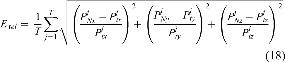
Suppose we take T sample points and n VGT modules for simulation. Then the relative error is calculated according to

\begin{array}{l} E_{r e l} = & \frac{1}{T} \sum_{j = 1}^{T} \sqrt{{(\frac{P_{N x}^{j} - P_{t x}^{j}}{P_{t x}^{j}})}^{2} + {(\frac{P_{N y}^{j} - P_{t y}^{j}}{P_{t y}^{j}})}^{2} + {(\frac{P_{N z}^{j} - P_{t z}^{j}}{P_{t z}^{j}})}^{2}} \end{array}

The absolute error is calculated by

\begin{array}{l} E_{a b s} = & \frac{1}{T} \sum_{j = 1}^{T} \sqrt{{(P_{N x}^{j} - P_{t x}^{j})}^{2} + {(P_{N y}^{j} - P_{t y}^{j})}^{2} + {(P_{N z}^{j} - P_{t z}^{j})}^{2}} \end{array}

According to the conclusion in subsection 3.3, suppose that the weight coefficients $k_{i} (i = 1, 2, \dots, 6)$ in the objective function are 0.005, the center of the obstacle $O_{m}$ locates at ${(400, 400, 400)}^{T}$ and the radius $L_{m}$ is equal to 300. We obtain ten end positions of the VGT manipulator with three and six modules, separately, as shown in Figures 7 and 8. The ten end positions with three modules are exactly the same as in Yang et al.²⁰ and the comparative results are shown in Table 3. They prove that the optimized end positions converge to the desired reference locations.

Figure 7.

(a) Position for X-axis with three modules; (b) position for Y-axis with three modules; (c) position for Z-axis with three modules.

Figure 8.

(a) Position for X-axis with six modules; (b) position for Y-axis with six modules; (c) position for Z-axis with six modules.

Table 3.

Comparison of simulation results with different method.

	Given positions	Our method	Method in Yang et al.²⁰	Our errors	Errors in Yang et al.²⁰
1	[2300,−150,−150]^T	[2296.18,−149.75,−149.75]^T	[2292.36,−149.50,−149.50]^T	3.8363	7.6726
2	[2350,−126,−126]^T	[2346.09,−125.79,−125.79]^T	[2342.19,−125.58,−125.58]^T	3.9213	7.8326
3	[2450,−115,−105]^T	[2445.90,−114.81,−104.83]^T	[2441.86,−114.62,−104.65]^T	4.1079	8.1564
4	[2500, −85,−100]^T	[2495.80,−84.86,−99.83]^T	[2491.69,−84.72,−99.67]^T	4.2058	8.3213
5	[2380,50,−120]^T	[2376.03,49.91,−119.80]^T	[2372.09,49.83,−119.60]^T	3.9761	7.9219
6	[2480,150,0]^T	[2475.85,149.75,−0.0038]^T	[2471.76,149.50,0]^T	4.1575	8.2552
7	[2560,0,0]^T	[2555.66,−0.0019,−0.0019]^T	[2550,0,0]^T	4.3400	10.0000
8	[2240,20,−20]^T	[2236.29,19.96,−19.97]^T	[2232.56,19.93,−19.93]^T	3.7103	7.4407
9	[2433,−128,59]^T	[2428.93,−127.79,58.90]^T	[2424.92,−127.57,−58.80]^T	4.0766	11.8078
10	[2356,−23,123]^T	[2352.08,−22.97,122.79]^T	[2348.17,−22.92,122.59]^T	3.9257	7.8411

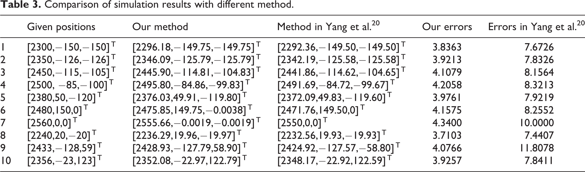
According to data from the simulation results, the relative error simulated under the condition of three modules is 0.2875%, and the absolute error is 4.0266 mm, which is reduced compared with Yang et al.²⁰ although the average running time is improved a little to 0.265 s. The corresponding errors and running times for a VGT manipulator with six modules are 0.2378%, 3.4576 mm and 0.745 s, respectively. However, when the VGT manipulator has many modules, the matrices K, M and F will become big, and solving the optimization problem will take relatively more time, so the algorithm has disadvantages for real-time operation of a large-scale VGT mechanical arm.

Conclusion

The inverse kinematics for an octahedral VGT manipulator were accomplished in this article. Based on the kinematics of the manipulator, we modeled the inverse kinematics problem as an optimization process, which we then solved. The optimization process was divided into two stages. The first stage determined each intermediate platform of the robot arm. The second stage worked out the corresponding actuator length according to the forward kinematics of the manipulator. We solved the minimization problem in the first phase by solving its Lagrange dual problem. Because the original optimization problem is strictly feasible, the Lagrange dual problem is a convex optimization. Thus, the solution we obtained is the globally optimal solution of the optimization problem. The simulation result illustrates the effectiveness of the proposed approach.

Footnotes

Declaration of conflicting interests

The author(s) declared no potential conflicts of interest with respect to the research, authorship, and/or publication of this article.

Funding

The author(s) disclosed receipt of the following financial support for the research, authorship and/or publication of this article: The research reported here was jointly supported by the National Natural Science Foundation of China (grant number 61374161) and China Aviation Science Foundation (grant number 20142057006).

Appendix

Proof: First, we rewrite equation (11) in the simplified form

where

As $f, f_{i}, g_{i}$ and $h_{i}$ are all second-order continuously differentiable real functions, we define a Lagrangian function of problem (20) as

\begin{array}{l} L^{*} (P, λ, u, v) = f (P) + λ f + u g + v h \end{array}

where

λ = [λ_{1}, λ_{2}, \dots, λ_{n}], u = [u_{1}, u_{2}, \dots, u_{n}], v = [v_{11}, v_{12}, \dots, v_{n m}]

are Lagrange multipliers, and

f = [f_{1}, f_{2}, \dots, f_{n}]^{T}, g = [g_{1}, g_{2}, \dots, g_{n}]^{T}, h = [h_{11}, h_{12}, \dots, h_{n m}]^{T}

are the quadratic constraints. Replace the above expressions into the Lagrange function

Apparently, matrix K is symmetrical, and hence, when $K > 0$ , it is to say that matrix K is positive definite and Lagrangian function $L^{*} (P, λ, u, v)$ is a convex function with respect to P. Then, by minimizing the function $L^{*} (P, λ, u, v)$ about P and letting $\nabla_{P} L^{*} (P, λ, u, v) = 2 K P + M^{T} = 0$ , the optimal solution can be achieved 22

\begin{array}{l} P^{*} = - \frac{1}{2} K^{- 1} M^{T} \end{array}

where

k_{i}, λ_{i}, u_{i}, v_{i}

satisfy

K > 0

and the corresponding Lagrange multipliers are denoted by

(λ^{*}, u^{*}, v^{*})

Then we obtain the Lagrangian dual function

In conclusion, the Lagrangian dual problem of (11) is

It is equivalent to solving the problem

According to the Schur complement (see Craig²⁴), the minimization problem of equation (23) can be rewritten as a convex optimization problem with LMI constraints

This problem can be efficiently solved by using the LMI toolbox. When $K > 0$ , the Lagrangian function $L^{*} (P, λ, u, v)$ is a convex function with respect to the design variable P. This ensures that the local optimal solution of the original problem is the global optimal one. Due to the established strong duality, if $(λ^{*}, u^{*}, v^{*})$ is the global optimal solution of the Lagrangian dual problem, then the corresponding solution $(P^{*}, λ^{*}, u^{*}, v^{*})$ is the global optimal one of the original minimization problem.

References

Miura

Furuya

Suzuki

. Variable geometry truss and its application to deployable truss and space crane arm. Acta Astronaut 1985; 12: 599–607.

Miura

Furuya . Adaptive structure concept for future space applications. IAA J 1988; 26: 995–1002.

Lee

Sanderson

. Dynamic analysis and distributed control of the tetrobot modular reconfigurable robotic system. Auton Robots 2001; 10: 67–82.

Badescu

Mavroidis

. Workspace analysis of reconfigurable robotic arms using parallel platforms as modules. In: Proceedings of ASME international mechanical engineering congress exposition, Washington, DC, 16–21 November 2003, pp.717–726. American Society of Mechanical Engineers (ASME).

Badescu

Mavroidis

. New performance indices and workspace analysis of reconfigurable hyper-redundant robotic arms. Int J Robot Res 2004; 23: 643–659.

Hanahara

Tada

. Variable geometry truss with SMA wire actuators (Basic consideration on kinematical and mechanical characteristics). In: 19th international conference on adaptive structures and technologies, Ascona, Switzerland, 6–9 October 2008, pp.96–100. Zurich: Swiss Federal Laboratories for Materials Science and Technology (Empa).

Rost

Uhlemann

Modler

. On the joint design and hydraulic actuation of octahedron VGT robot manipulators. In: IEEE/ASME international conference on advanced intelligent mechatronics, Wollongong, Australia, 9–12 July 2011, pp.92–97. Piscataway, NJ: IEEE/ASME.

Chirikjian

Burdick

. A hyper-redundant manipulator IEEE Robot Autom Mag 1994; 1: 22–29.

Chirikjian

Burdick

. Kinematically optimal hyper-redundant manipulator configurations. In: IEEE international conference on robotics and automation, Nice, France, 12–14 May 1992, pp.415–420. New York: IEEE.

10.

Fahimi

Ashrafioun

Nataraj

. An improved inverse kinematic and velocity solution for spatial hyper-redundant robots. IEEE T Robotic Autom 2002; 18(1): 103–107.

11.

Zanganeh

Angeles

. The inverse kinematics of hyper-redundant manipulators using splines. In: IEEE international conference on robotics and automation, Nagoya, Japan, 21–27 May 1995, vol. 3, pp.2797–2802. New York: IEEE.

12.

Bayram

Ozgoren

M K

. The conceptual design of a spatial binary hyper-redundant manipulator and its forward kinematics. Proceedings of the Institution of Mechanical Engineers, Part C: Journal of Mechanical Engineering Science 2012; 226: 217–227.

13.

Bayram

Ozgoren

M K

. The position control of a spatial binary hyper-redundant manipulator through its inverse kinematics. Proceedings of the Institution of Mechanical Engineers, Part C: Journal of Mechanical Engineering Science 2013; 227: 359–372.

14.

Iwatsuki

Nishizaka

Morikawa

. Motion control of hyper-redundant manipulator built by serially connecting many parallel mechanism units with a few DOF. Int J Autom Tech 2010; 4: 364–371.

15.

Mintenbeck

Estanna

. Design modelling and control of a hyper-redundant 3-RPS parallel mechanism. In: IEEE international conference on robotics and biomimetics, Tianjin, China, 14–18 December 2010, pp.591–596. New York: IEEE.

16.

Chibani

Mahfoudi

Chettibi

. Generating optimal reference kinematic configurations for hyper-redundant parallel robots. P I Mech E–I J Sys 2015; 229.

17.

Bilbao

Avilĺę

Aguirrebeitia

. Eigensensitivity-based optimal damper location in variable geometry trusses. AIAA J 2009; 47: 576–591.

18.

de Zĺćrate

I O

Aguirrebeitia

Avilĺę

. A method for the inverse dynamics analysis of variable geometry trusses. ICNAAM 2010: international conference of numerical analysis and applied mathematics (eds Simos

Psihoyios

Tsitouras

), Rhodes, Greece, 19–25 September 2010, vol. 1281, pp.1275–1280. American Institute of Physics Publishing.

19.

Rost

Uhlemann

Modler

20.

Yang

Jiang

. Fast trajectory planning for VGT manipulator via convex optimization[J]. Int J Adv Robot Syst 2015; 12.

21.

Chirikjian

. Inverse kinematics of binary manipulators using a continuum model. J Intell Robot Syst 1997; 19: 5–22.

22.

Williams

. Kinematic modeling of a double octahedral variable geometry truss (VGT) as an extensible gimba. NASA Technical Memorandum, 1994.

23.

Craig

JJ.

Introduction to robotics: Mechanics and control. 3 rd ed. Upper Saddle River: Pearson Prentice Hall, 2004.

24.

Boyda

Vandenberghe

. Convex optimization. 1st ed. New York: Cambridge University Press, 2004.

Inverse kinematics for the variable geometry truss manipulator via a Lagrangian dual method

Abstract

Keywords

Introduction

Kinematic analysis of the VGT manipulator

Inverse kinematic modeling

Backbone curve modeling

Formulation of the optimizing process

Boundary conditions and physical limitations

Obstacle avoidance

Problem statement and solution

Numerical simulations

Kinematics of single VGT module

Simulation results

Conclusion

Footnotes

Declaration of conflicting interests

Funding

Appendix

References