
Abstract
Exact motion estimation is one of the major tasks in autonomous navigation. Conventional Global Positioning System-aided inertial navigation systems are able to provide accurate locations. However, they are limited when used in a Global Positioning System-denied environment. In this paper, we present a square root unscented Kalman filter-based approach for navigation by using stereo cameras and an inertial sensor only. The main contribution of this work is the development of a novel measurement model by applying multiple view geometry constraints to the stereo cameras/inertial system. The measurement model does not require the three-dimensional feature position in the state vector of the filter, which substantially reduces the size of the state vector and the computational burden. To incorporate this nonlinear and complex measurement model, a variant of the square root unscented Kalman filter-based algorithm is also proposed. The root of the state covariance is propagated and updated directly in the square root unscented Kalman filter, thereby avoiding the decomposition of the state covariance and improving the stability of our algorithm. Experimental results based on a real outdoor dataset are presented to demonstrate the feasibility and the accuracy of the proposed approach.
Keywords
Introduction
In recent years, the inertial measurement unit (IMU) has been widely used for the navigation tasks of robots, cars, unmanned aerial vehicles, and so forth, thanks to the remarkable advances in Micro-Electro-Mechanical System (MEMS) inertial sensors, such as lower cost, smaller size, lighter weight, higher power efficiency, etc. The IMU-based inertial navigation system (INS) is able to track fast motion with high precision in a short period of time. However, the accuracy of INS deteriorates with time because of the accumulative error caused by sensor biases and noises. A conventional method to tackle this problem is using the Global Positioning System (GPS) to correct the error of INS periodically. A major limitation of the approach is that the GPS/INS system cannot be used in GPS-denied environments where GPS receivers do not function, 1 such as indoors, forests, and underground. Besides, high precision GPS receivers are usually expensive and bulky.
An alternative approach to restrain the IMU error is the use of visual sensors such as stereo cameras. Both position and attitude information could be extracted by tracking visual features between sequences of images captured from cameras. The estimation accuracy in such a system depends on the observed scene instead of the accumulative time, and the visual motion estimation achieves high accuracy in a slow motion scenario. For this reason, the fusion of visual and inertial sensors has garnered considerable attention from many researchers. Peter Corke 2 presents a tutorial introduction of inertial and visual sensing from a biological and engineering perspective. A set of algorithms of relative pose (translation and rotation) calibration for hybrid inertial/visual system can be found in Lang and Pinz, 3 Lobo and Dias, 4 and Mirzaei and Roumeliotis. 5 Since this paper is mainly concerned about navigation, we focus on the data fusion algorithm of inertial and visual sensors for motion estimation.
An area of particular relevance to our work is visual odometry, which focuses on the use of either monocular or stereo vision to estimate the ego-motion of an agent with respect to the environment. For the monocular case however, the detected feature suffers from the issue of scale unobservability. To overcome the problem, Feng et al. 6 and Davison et al. 7 employ the fixed depth constraint, whilst a delayed feature initialization scheme is presented in Davison 8 and Kim and Sukkarieh. 9 The stereo cameras, inherently, are able to provide scale through the baseline between the cameras. This is demonstrated by Davison and Murray 10,11 in the presented active stereo visual Simultaneous Localization And Mapping (SLAM) systems. Nevertheless, the vision-only techniques highly depend on the available features, causing difficulties in recovering the real track when all tracked features are lost.
In order to overcome the limitations of vins vision-only techniques, numerous work has been reported recently about hybrid stereo cameras and inertial systems. A Kalman filter (KF) is employed in Kelly et al. 12 and Carillo et al. 13 to fuse stereo visual odometry and inertial measurements for the estimation of unmanned aerial vehicle position and velocity. As a loosely coupled approach, it does not utilize inertial sensors in the prediction of the tracked features. A tightly coupled approach is often preferable since it makes better use of information from these two sensors. Veth and Raquet 14 develop an image-aided inertial navigation algorithm on the basis of a multi-dimensional stochastic feature tracker. An unscented KF (UKF)-based filter for localization, mapping, and self-calibration of inertial and visual sensors is presented in Kelly and Sukhatme. 15 In order to tackle the far and near features in large-scale outdoor environments, Xian 16 proposes an (iterative extended KF) IEKF-based tightly coupled integration algorithm using stereo cameras and a low-cost IMU. In these tightly coupled approaches, the positions of the features are contained in the filter. However, one of the main demerits of these approaches is the growing state space maintained within the filter along with the increase in the number of the features, resulting in a higher computational burden.
A remedy to this issue is presented in Diel et al. 17 and Nilsson et al., 18 where the epipolar geometry between current and previous images is used and combined with the IMU measurement. Also, in Mourikis and Roumeliotis, 19 the authors present an extended KF (EKF)-based algorithm for vision-aided inertial navigation. Although three-dimensional (3D) feature positions are removed from the vector of the filter state, it still makes use of a least-square solution to estimate the 3D position of feature points. In Indelman et al., 20 both epipolar and three-view geometry constraints are used for monocular and inertial sensor integration. A similar approach could be found in Hu and Chen. 21 The difference is that the former uses an EKF while the latter employs a UKF. The standard UKF utilizes the Cholesky decomposition in order to generate the sigma points at each time step. However, the main flaw of this approach is that the Cholesky decomposition may become unstable, especially when the covariance matrix becomes negative. The square root UKF (SRUKF), a re-implementation of the general UKF presented by Van Der Merwe and Wan, 22 is able to achieve exactly the same accuracy. Yet, it avoids the decomposition process by directly propagating the Cholesky factor instead of the covariance of the state. Compared with EKF, the SRUKF/UKF has precision to the third order while the EKF is accurate to the first order only for the Gaussian state distribution. 23 Besides, the SRUKF/UKF is derivative-free, which means that the filter does not require the computation of Jacobian matrices.
In this paper, we propose a novel multiple view geometry constraints-based measurement model by applying the epipolar and trifocal geometry constraints to stereo vision. The stereo-vision-based approaches only require the previous and current moments to employ the three-view/trifocal geometry, compared with at least three moments in the monocular approaches. 20,21 Besides, the stereo cameras inherently contain the depth information, which will help improve the position estimation. The main benefit of using the measurement model is that the 3D position of the feature does not need to be contained in the state vector of the filter, resulting in less storage space and computational burden. Furthermore, an improved SRUKF algorithm is proposed in our approach for the purpose of fusing the stereo camera information with the inertial measurement. To improve the robustness and accuracy of the estimation, our approach employs a two-step method to reject outliers, which consists of an epipolar constraint check for left–right outlier removal and a random sample consensus (RANSAC) algorithm for previous–current outlier rejection.
The remainder of the paper is organized as follows. The process model and measurement model are detailed in the second section. In the third section, the background of the SRUKF is briefly introduced and its improved version in our approach is also presented. Multiple trails from a real dataset are used to evaluate our algorithm, with their results presented in he fourth section and Appendix. Finally, the main conclusions are drawn in the fifth section.
System modeling
Reference frames
The goal of this paper is to estimate the pose of an carrier with respect to the world frame by integrating stereo cameras and an IMU. Three reference frames are used, as shown in Figure 1.

The reference frames and their relationship. The yellow solid line between two frames represents a fixed connection while the yellow dashed one denotes a flexible connection. The two camera frames CL, CR and the IMU frame I are rigidly attached. The features points M are modeled in the world frame W.
The world frame W: The pose of the IMU is estimated with respect to this frame, which is anchored to the earth. The features (like the feature point M shown in Figure 1) in the scene are modeled in this frame. It can be aligned in any way; however, in this paper it is defined as vertically aligned, with the x, y, and z-axis being aligned with the east, north, and up direction, respectively.
The camera frame C: This frame is attached to the moving stereo cameras, with its origin placed at the optical center of the camera, and with the z-axis pointing along the optical axis. There are two camera frames, as shown in Figure 1, and they are aligned with each other with a known translation. In this paper, we choose the left camera as the reference camera frame.
The IMU frame I: This is the frame of the IMU, with its origin at the center of the IMU body. The x, y, and z-axis respectively denotes the front, left, and up direction of the IMU body.
The camera frame and IMU frame are rigidly attached. The features are modeled in the world frame and assumed to be static. The assumption may not always be true in practice, for there may be some moving objects in the scene, such as running cars and walking pedestrians. In such a circumstance, these moving features can be rejected by the RANSAC algorithm in the proposed approach, which will be detailed in a later section. Since the pose of the IMU is variable with respect to the world frame, the estimation of the IMU pose is the main objective of this paper.
State representation
The state vector used in the proposed approach consists of the current IMU-related state vector and the last pose of IMU, that is

where qWI is a unit quaternion
24
which denotes a rotation quaternion from frame I to frame W;
The state in equation (1) is not estimated in the SRUKF directly. The error-state is estimated in the filter and then used to compensate the state. Following equation (1), the error state is defined as follows

For the IMU position, velocity, and biases, the error is defined as

where the operator of ⊗ denotes quaternion multiplication. It is worthwhile to note that the attitude error δ
Process model
The process model describes the time evolution of the state. In our approach, the biases of inertial sensors

As for the error-state, the propagation can be deduced from state propagation equations and the definition of the error-state. Here we present the error-state process model directly. Interested readers could refer to Xian et al. 16 for details.

where

Multiple view constraints-based measurement model
The measurement used in this paper is the multiple view geometry constraint between two consecutive stereo image pairs, or more precisely, the epipolar constraint and the trifocal tensor constraint. Both previous and current stereo images are taken into consideration. Assume the left and right images in the previous view are denoted respectively by Im1 and Im2, and these in the current view are denoted by Im3 and Im4. In our case, the epipolar constraints used for measurement are the pairs (Im1, Im3) and (Im2, Im4), out of in total six combinations. These two pairs are chosen because they contain the relative pose information between the previous and current poses, which is helpful to improve the accuracy of the state estimates. Similarly, the trifocal tensor constraints used in the measurement are groups (Im1, Im2, Im3) and (Im1, Im2, Im4).
The epipolar geometry describes the intrinsic projective geometry between two views, which is independent of scene structure, and only depends on the cameras’ internal parameters and relative pose.
Suppose a point M in the 3D-space is imaged in two image planes, at

The epipolar geometry constraint between two views.
In terms of the three views geometry, it has similar properties; it is independent of the scene structure and only depends on the projective relations between the cameras. The new ability of the tri-view geometry compared with the two-view case is capable of transferring from two views to a third. As shown in Figure 3, line The point-line-point correspondence between three views.

The trifocal tensor

Applying the two geometry constraints to our case, the measurement model can be presented as

where
Square root unscented Kalman filter-based implementation
As for the fusing method, a variant of the SRUKF is used for integrating stereo images and the inertial measurement, since it has an excellent capacity for dealing with nonlinear problems and superior performance when compared with the EKF and UKF. State prediction and measurement update are the two main steps of the SRUKF. In order to predict state, the standard SRUKF requires the sigma point to be calculated; however, in our approach, we predict the state directly based on our process model. In this approach, less computation is needed. To implement the SRUKF, two linear algebra techniques are used, namely QR decomposition and Cholesky factor updating.
State prediction
In our case, the state prediction process is different from the standard SRUKF. The state is predicted based on the process model. Assume that the state and the Cholesky factor at time k is respectively


where
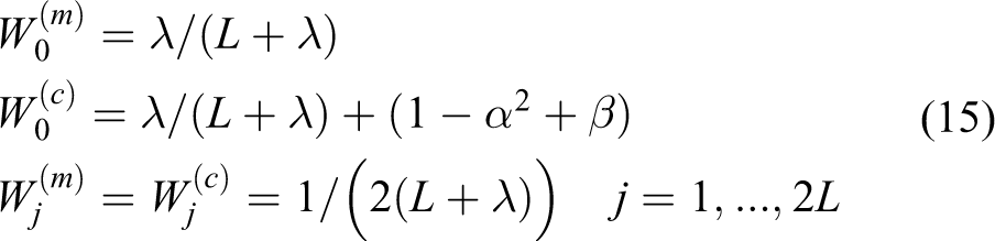
Measurement prediction and update
To calculate the statistics of measurement

where L is the dimension of the state, in our case L = 21,

where
The sigma vector of the measurement then can be obtained through the nonlinear measurement function

The mean and the Cholesky factor of the measurement prediction is approximated as follows


The measurement update equations are
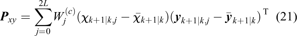


where
Feature detection, tracking, and outlier rejection
Feature detection and tracking are vital steps for visual odometry, visual/inertial integration, and many other vision applications. In recent decades, a variety of methods have been proposed. Fraundorfer and Scaramuzza 28 compared the properties and performance of several popular feature detectors, such as FAST corner detection (FAST), 29,30 Scale Invariant Feature Transform (SIFT), 31 and Speeded-Up Robust Features (SURF). 32 In Desai and Lee, 33 the authors compared recently developed Binary Robust Independent Elementary Features (BRIEF) 34,35 and Binary Robust Invariant Scalable Keypoints (BRISK), 36 and presented a novel feature descriptor called SYnthetic BAsis (SYBA) 37,38 for accurate feature matching. In our visual/IMU approach, we mainly focus on the integration method of visual and IMU information. As for the feature detection algorithm, a fast, efficient, and sophisticated algorithm is welcomed. So we employ the FAST detector for detecting corner features in the image. The major advantage of the FAST algorithm is its high efficiency in reaching accurate corner localization in an image. For feature tracking, the Kanade Lucas Tomasi (KLT) tracker 39 is used. The KLT tracker allows tracking features over long image sequences and undergoing larger changes by applying an affine-distortion model to each feature.
However, matched points are usually contaminated by outliers due to image noise, occlusion, image blur, and changes in viewpoint. In this paper, a two-step method is introduced to reject the outliers. First, we use the epipolar geometry constraint for left–right outlier removal. If we take
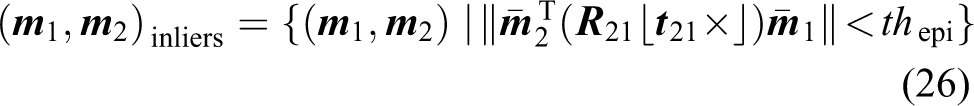
where thepi is the threshold for the epipolar constraint.
It is then followed by the RANSAC algorithm for the past–current outlier rejection. To implement the RANSAC algorithm, the trifocal tensor constraint is used. Taking the features in the Im1, Im2, and Im3 as an example, we reject the outlier by using the formula below

where thtri is the threshold for the trifocal tensor constraint.
Experimental results
To evaluate the performance of the proposed algorithm, the KITTI dataset 40 is used. This dataset is available to the public and was chosen because it contains easy-to-process data from various types of sensors. The recording platform is equipped with two grayscale cameras, two color cameras, a rotating 3D laser scanner, and a combined GPS/IMU INS. Two versions of data are provided: raw (unsynced + unrectified) and processed (synced + rectified).
Since we focus on navigation tasks based on stereo and inertial sensors, we used the unsynced IMU measurements sampling at 100 Hz and the rectified grayscale stereo sequences sampling at 10 Hz. The pixel resolution of the rectified images is 1226×370. To synchronize the measurements from the IMU and cameras, we minimize the timestamp difference between the two types of measurements, resulting in synchronization errors no greater than 5 ms. The result of the GPS/IMU integrated system is used as the ground truth, as it provides open sky position/attitude precision as high as 0.02 m/0.1 deg.
We have tested our algorithm with most of the KITTI data and compared it with the pure inertial navigation solution, stereo visual odometry, 41 and the UKF-based monocular aided inertial navigation solution (UKF-Mono/IMU). 21 The results shown in this section are a typical representative of many trials. Additional test results can be found in the Appendix. The trajectory of the trail is about 4.1 km, taking 518 s with the average velocity of about 8 m/s. The initial attitude, speed, and position of the filter are provided by the results of GPS/IMU.
Trajectory estimation and comparison
The estimated trajectories are overlaid on the Google map as shown in Figure 3, and the corresponding two-dimensional (2D) horizontal position errors are depicted in Figure 3. Note that the large error from 75 s to 120 s is caused by ground truth error. For this reason, we do not take the period (75–120 s) into consideration when calculating the root mean square error (RMSE), the maximum error (MAXE), and the end-point error (ENDE). The overall RMSE, MAXE, and ENDE are shown in Table 1. Clearly, the worst one is the pure inertial navigation solution, with the end position error of about 21 km. The inertial navigation is actually an integral process (the position is computed through quadratic integral while the attitude is obtained by single integral), and therefore even a little sensor bias or noise error accumulates quickly, resulting in quadratic position error over time. This is the main reason why a low-cost INS usually needs to be aided by other types of sensors. As for the results of stereo visual odometry, the solution is found to be better than that of the inertial-only solution. The trajectory estimated by stereo visual odometry has high accuracy in the beginning, but the heading error increases gradually over time, resulting in the maximum position error of about 160 m.
Horizontal position error comparison

UKF: unscented Kalman filter; IMU: inertial measurement unit; SRUKF: square root unscented Kalman filter; RMSE: root mean square error; MAXE: maximum error; ENDE: end-point error.
Compared with the pure inertial navigation solution and stereo visual odometry, both the UKF-VINS (Visual aided INS) and our proposed method have much better performance. It also shows the advantage of the combination of inertial and visual sensors. Both UKF-VINS and our proposed method are the visual aided inertial navigation approach and use the trifocal tensor geometry as measurement information. The main difference is that the UKF-VINS combines the monocular camera and the inertial sensor based on the UKF, while our proposed method fuses stereo cameras and the inertial sensor based on the SRUKF. As shown in both Figure 4 and Table 1, our proposed method has less position error and better accuracy than UKF-VINS.

Comparison of trajectory estimation. (a) An overview of trajectory overlaid on the road map. (b) Horizontal position errors of different solutions. Noteworthy is the fact that the position estimated by GPS/IMU (the black dashed ellipses in both (a) and (b)) has large errors in some areas, probably due to loss of GPS satellites.
Velocity and attitude estimation and comparison
The velocity and attitude estimated by our proposed method are compared with that of the UKF-VINS. The results of the pure inertial navigation solution and stereo visual odometry are not used for comparison here, since their performance is much more poor, and the stereo visual odometry can not provide velocity directly. The velocity and attitude errors are compared in Figure 5 and the corresponding RMSE and MAXE are shown in Table 2. The jumps appearing in Figure 4 are again because of the loss of GPS signal. According to Figure 5 and Table 2, it is clear to see that the velocity and attitude estimations by our proposed method have higher accuracy than that of UKF-VINS, with the accuracy being better than 0.5 m/s for velocity RMSE and better than 1 deg for attitude RMSE in this experiment.
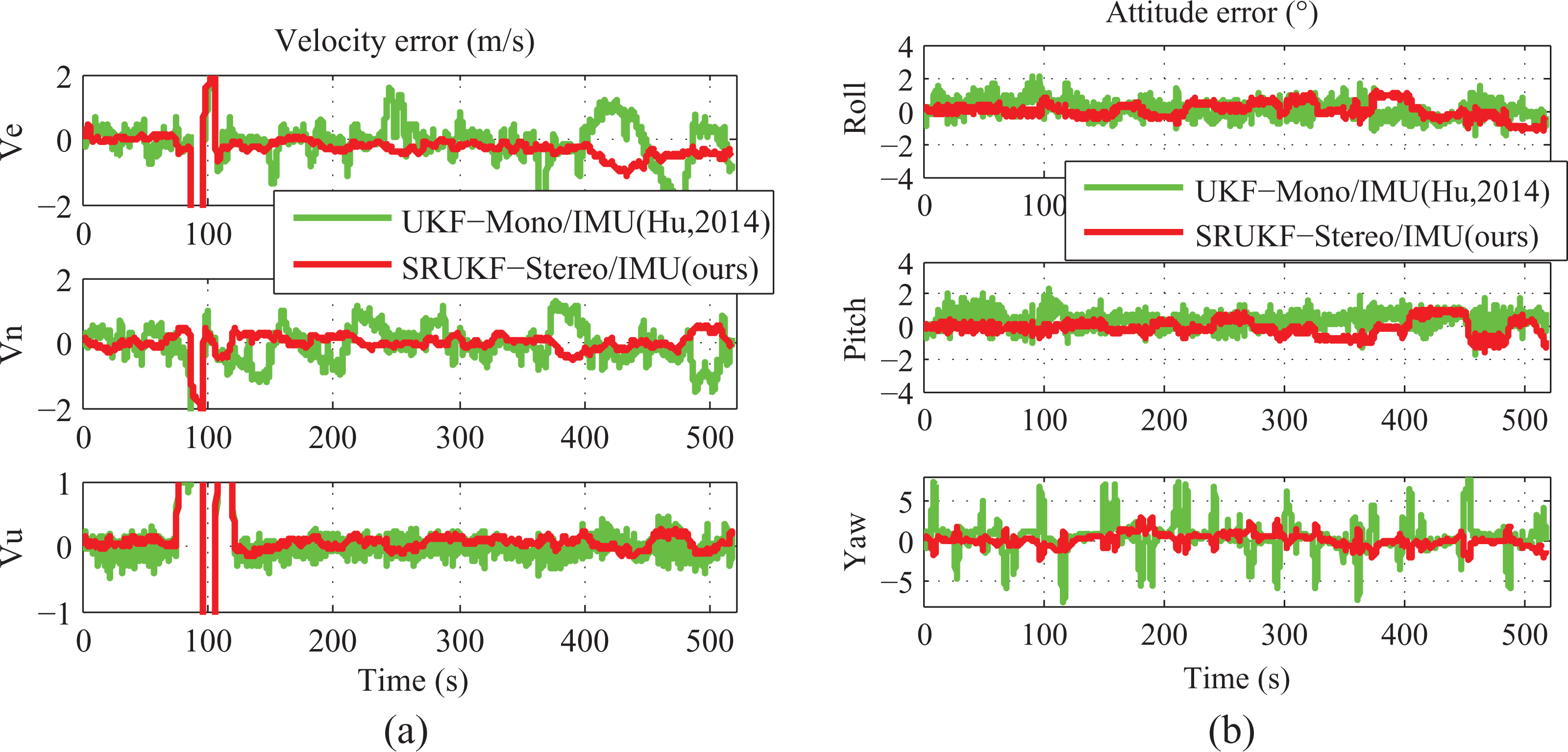
Velocity error (a) and attitude error (b) comparison. The large error appearing in (a) from about 75 s to 120 s is caused by the GPS outage, which can be seen in Figure 4; Ve: East Velocity; Vn: north velocity; Vu: up velocity.
Velocity and attitude error

Results of feature tracking and outlier rejection
The positions of tracked features from the image sequence are not included in our filter, but are used as the measurement. The quality of the feature plays an important role in our algorithm. During feature tracking, we set a reference feature number of 80 in our case. Once the feature quantity is less than the value, new features are added into the filter. As shown in Figure 6(a), the average number of features is about 80. The tracked features are selected by our RANSAC approach; the moving objects (the features in the yellow ellipse shown in Figure 6(a)) are rejected effectively. The inlier rate of the test is also shown in Figure 6(b). Most of the time, the inlier rate is above 0.8, which is an important guarantee for reliable integration. It is worth mentioning that the inlier rate becomes zero in the time of frame ∼200, as shown in Figure 6(b). This is mainly caused by the large time difference between the IMU and the camera while the vehicle is moving at a high speed in the test. When this issue occurs, the pose could be updated by using the INS only, demonstrating the higher reliability of the inertial/visual approach in particular circumstances.

Image features and inlier rate. (a) Two sample images and tracked features. (b) Feature number and inlier rate of this particular experiment. The detected features are shown in the images in (a), the green ones are inliers while the red ones are outliers.
Conclusions
In this paper, we present an SRUKF-based stereo camera and inertial sensor integration architecture for autonomous navigation. As we put our focus on the navigation and location rather than the environment reconstruction, the 3D positions of the features are not included in the filter. The measurement of the filter utilizes the multiple view geometry constraints (to be exact, the epipolar constraint and the trifocal tensor geometry constraint) between the consecutive two image pairs. The system model, the implementation of the SRUKF-based algorithm, and the feature detection, tracking, and outlier rejection method are presented in this paper.
The proposed algorithm has been validated using real outdoor data. The experiment results are compared with the pure inertial navigation solution, stereo visual odometry, and UKF-Mono/IMU approaches. The comparison shows that the proposed algorithm has multiple orders of magnitude improvement than the pure inertial navigation solution, and has more precise location and heading estimation than the stereo visual odometry and UKF-Mono/IMU approaches. The results also show the effectiveness of the outlier rejection method, which is able to reject the moving objects in the scene. The maximum 2D horizontal position error is less than 20 m for the typical vehicle path of about 4.1 km. It is concluded that the proposed algorithm has a precise motion estimation performance and is able to be used in GPS-denied environment.
Footnotes
Declaration of conflicting interests
The author(s) declared no potential conflicts of interest with respect to the research, authorship, and/or publication of this article.
Funding
The author(s) disclosed receipt of the following financial support for the research, authorship and/or publication of this article: This work was supported by the National Natural Science Foundation of China (grant number 61503403, 61573371) and National University of Defense Technology Advanced Research Programs (grant number JC14-03-04, JC14-03-06)
Appendix: Results of other trails
The algorithm is also tested with other four trails. The estimated positions, attitude errors, and velocity errors are presented and compared in Figure 7. The video clips of all our results are available online.