Analysis and optimization of a camber morphing wing model

Abstract

This article proposes a camber morphing wing model that can continuously change its camber. A mathematical model is proposed and a kinematic simulation is performed to verify the wing’s ability to change camber. An aerodynamic model is used to test its aerodynamic characteristics. Some important aerodynamic analyses are performed. A comparative analysis is conducted to explore the relationships between aerodynamic parameters, the rotation angle of the trailing edge, and the angle of attack. An improved artificial fish swarm optimization algorithm is proposed, referred to as the weighted adaptive artificial fish-swarm with embedded Hooke–Jeeves search method. Some comparison tests are used to test the performance of the improved optimization algorithm. Finally, the proposed optimization algorithm is used to optimize the proposed camber morphing wing model.

Introduction

Airplanes have played an important role in history since the first airplane was invented in 1903. Developments in science and technology have led to more advanced airplane structures that offer higher efficiency, lower cost, greater maneuverability, the ability to cruise, and so forth. In recent years, the study of airplane wings has become a hot topic, with particular interest in camber morphing wings ^{1 –3} as shown in Figure 1.

Figure 1.

Diagram of a camber morphing wing model.

Civilian airplanes consume large amounts of fuel during a flight. The weight of fuel accounts for more than 30% of the airplane’s total weight. ⁴ A camber morphing wing with a variable camber trailing edge reduces fuel consumption by at least 5% and increases the lift coefficient from 0.08 to 0.4. ⁵ For business jets in America, this could translate into a saving of US$7 billion a year. ⁶

Fighter aircrafts are the main weapon of a military air force. Fighter aircrafts are a focus of national defense technology research. A high-performance fighter aircraft must have high maneuverability, strong adaptability, and super invisibility to adapt to different combat situations. Traditional fighter aircrafts have a flap at the end of the wing that improves the aerodynamic characteristics. However, when the flap changes its angle, it leaves a gap between the wing and the flap. This gap reduces the invisibility of fighter aircrafts and makes the airflow above the wing separate in advance, which has a negative effect on the aerodynamic characteristics. ⁷

A camber morphing wing with a morphing trailing edge can change the camber of the trailing edge continuously, thereby improving the aerodynamic characteristics. The flight test results indicate that a camber morphing wing can reduce resistance by 7% when the airplane is in a cruise state, by 6% when it is in a fatigue state, and by more than 20% when it is in a high-speed cruise state. ⁷ Therefore, research on camber morphing wings has very important scientific and realistic significance.

In 1993, Rossi et al. ⁸ investigated the use of an active rib to control the shape of an adaptive morphing wing. The morphing wing consisted of many parts and external linear variable differential transformers, but it was too complex and heavy. In 2000, Monner et al. ⁵ proposed an elastic trailing edge for an adaptive morphing wing. The wing rib consisted of many flexible sections and the elastic trailing edge could change its camber continuously. However, the trailing edge used prismatic joints that could easily become locked. In 2004, Maute and Reich ⁹ used an aeroelastic topology optimization approach to design an adaptive morphing wing. The designed model attracted substantial attention in the microelectromechanical systems community. However, the camber for the morphing trailing edge did not change continuously. In 2009, Marques et al. ¹⁰ designed a morphing trailing edge for minimum drag and improved energy efficiency. Although this wing had improved aerodynamic characteristics, the camber did not change continuously. In 2011, Vos and Barrett ¹¹ applied a pressure-adaptive honeycomb to the design of a morphing wing. The experimental data indicated that the structure achieved better aerodynamic characteristics. However, the control of the pressure-adaptive honeycomb was difficult and complex and its application needs time.

Structure optimization is an important part for mechanisms. There are many optimization algorithms such as Newton method, conjugate gradient method, Sequential Quadratic Programming (SQP), simplex method, and so on. But these methods are based on strict mathematic models. When the dimensions of variables, the number of constraint equations, and nonlinearity are complex or the model can’t be expressed by explicit functions, problems will not be effectively solved by these methods. ¹² Since 1940s, people have drawn inspiration from biological systems to solve many practical problems and proposed many intelligent bionic optimization algorithms such as genetic algorithms (GA), ¹³ ant colony optimization (ACO), ¹⁴ artificial immune algorithm (AIA), ¹⁵ particle swarm optimization (PSO), ¹⁶ and so on. All these algorithms have the function of global optimization. But there are also some disadvantages for each algorithm. GA and AIA are still limited by the dimensions of variables and these need some skills to use them just like the coding problem of GA. ^17,18 Compared with other intelligent algorithms, the computation time of ACO is longer and it is easy to appear stagnation behavior. ¹⁹ For PSO, if the momentum coefficient is very large, the optimal solution may be missed. In the final period, the convergence velocity is slow which make the algorithm to lose accuracy. ²⁰ In 2003, a scholar proposed a new intelligent optimization algorithm called artificial fish swarm (AFS) algorithm. ²¹ This method has good ability to overcome local extremum values and obtain global optimal solution. This algorithm only uses the function values of the target function, without special information, such as gradient values of the objective function. It also has powerful self-adaptive ability in the search space, because there is no request for initial values. It is not sensitive to parameter selection. ²² But there are also some disadvantages for this algorithm such as search visual and iteration step are constant, the random search in prey action with low efficiency, and so on. ²³ Because of the excellent performance of AFS, this article shows some improvement on it and the optimization of its structure.

This article is structured as follows. Section “Structure design of a camber morphing wing model” proposes a camber morphing wing mechanism. Section “Kinematic simulation and aerodynamic analysis” sets up the mathematical model for the mechanism and finishes the kinematic simulation. An aerodynamic model is set up and some important aerodynamic analysis has been done. Section “Weighted adaptive AFS optimization algorithm with embedded Hooke–Jeeves search method” proposes an improved optimization algorithm and investigates its performance. Then this article uses this method to optimize the proposed morphing wing. The conclusions and future work are presented in the section “Conclusion.”

Structure design of a camber morphing wing model

Many studies have investigated the camber morphing wings. ^{3,24 –29} Most of these studies focus on new intelligent materials, although the control of them is complex and difficult. ^{30 –32} In contrast, the planar linkage mechanism has a long history and has many advantages. For example, low pairs are used to connect with bars, making the whole mechanism reliable and stable, increasing the mechanism’s carrying capacity, and providing excellent wear resistance. Planar linkage mechanisms can achieve various forms of movement. Because the structures of low pairs are not complex, the manufacturing process is relatively easy and accurate. Therefore, this study makes full use of planar linkage mechanisms with traditional materials to design camber morphing wings.

Because camber morphing wings can change the shape, there must be a camber. Therefore, the design scheme shown in Figure 2 is proposed.

Figure 2.

Proposed camber morphing wing model: (a) Diagram of the design scheme and (b) the 3-D model of the design scheme. 3-D: three-dimensional.

In Figure 2(a), there are three closed loops and 12 bars. Bars AB, BC, CD, AD, EF, DG, GH, IJ, GK, and KL are binary links. Bars FCH and JHL are ternary links. The degree of freedom (DOF) of the structure is $3\times (12-1)-2\times 16=1$ . Figure 2(b) is the three-dimensional model of the design scheme. Different parts have different colors. An input to bar BD drives the first closed loop and the output is on bar FCH that drives the second closed loop, and so on. This structure is lighter than the structure proposed by Monner. ⁴ The morphing trailing edge proposed by Monner ⁴ uses metal plates to form the mechanism. In each section, there are three solid metal plates. If there are n sections, the total number of metal plates is 3n. However, the morphing trailing edge proposed in this article uses planar linkages to form the mechanism. If the corresponding sections of the two different morphing trailing edges have the same size and the thickness of the linkages and plates are same, the weight of the model proposed in this article is less than the weight of the model proposed by Monner. ⁴ Therefore, from the weight perspective, the structure in this article is improved. The detailed design process for the structure proposed in this article is described below.

A morphing wing must be able to change its camber according to different working conditions. The deformation of the back closed loop must be greater than that of the front closed loop, which requires a mechanism that can amplify and deliver deformation. The current design uses a lever mechanism. When the fulcrum is located at the left or right end point of the horizontal bar and the input is located at the midpoint of the horizontal bar, the output is amplified. When the fulcrum is located at the midpoint and the input is located at the left or right end point, the output is reversed. A lever mechanism is inserted into two different closed loops, as shown in Figure 3.

Figure 3.

Morphing trailing edge with two closed loops.

In Figure 3, the lever mechanism is made up of bar FCH and bar CD. Because there are no fixed points, point F is used as the equivalent fulcrum. Assume that there are two inputs, D₁ and D₂, located on points F and C, as shown in Figure 4. If $D_1<D_2$ , there will be a relative displacement between F and C. The output at point H is amplified. Therefore, the mechanism shown in Figure 4 has the same effect as a lever mechanism.

Figure 4.

Diagram of the equivalent lever.

When the bar rotates around the fixed point B, the vertical displacement of point D is larger than that of point E. Therefore, there are two orthokinetic inputs with different magnitudes. Point H then receives an orthokinetic and amplified output. The deformation of the second closed loop is greater than that of the first closed loop, which generates a camber. The assembly process is shown in Figure 5.

Figure 5.

The assembly process of the camber morphing wing model.

Kinematic simulation and aerodynamic analysis

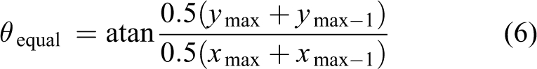
The design scheme is put into the plane rectangular coordinate system as shown in Figure 6(a). Assume that θ is the angle between BD and B′ D′. In this article, clockwise is positive. When there is no camber change, the labels of the points are A, B, C, D, E, F, G, H, I, J, K, and L; otherwise, the corresponding labels are A′,B′, C′, D′, E′, F′, G′, H′, I′, J′, K′, and L′. Assume that θ_equal is the angle between the x axis and the line whose endpoints are the midpoint of KL and the origin of the coordinate as shown in Figure 6(b).

Figure 6.

The design scheme in the rectangular plane coordinate system: (a) all the points and (b) equal.

The known conditions are $l_{\text{AB}},l_{\text{KL}},l_{\text{total}},\gamma$ , and $\beta .l_{\text{total}}$ represents the total length of the trailing edge without any camber change. γ represents the angle between AC and the x axis: $\angle \text{FCH}=\angle \text{JHL}=\beta$ . Then, it is easy to obtain the coordinates of A′,B′, D′, and E′.

To obtain the coordinates of C′,F′, G′, and J′, the following nonlinear equations can be set up

$\{\begin{array}{c}{\left(x_{\text{C′}}-x_{\text{D′}}\right)}^2+{\left(y_{\text{C′}}-y_{\text{D′}}\right)}^2={\left(l_{\text{D′C′}}\right)}^2\\ {\left(x_{\text{C′}}-x_{\text{A′}}\right)}^2+{\left(y_{\text{C′}}-y_{\text{A′}}\right)}^2={\left(l_{\text{A′C′}}\right)}^2\end{array}$

1

$\{\begin{array}{c}{\left(x_{\text{F′}}-x_{\text{C′}}\right)}^2+{\left(y_{\text{F′}}-y_{\text{C′}}\right)}^2={\left(l_{\text{F′C′}}\right)}^2\\ {\left(x_{\text{F′}}-x_{\text{E′}}\right)}^2+{\left(y_{\text{F′}}-y_{\text{E′}}\right)}^2={\left(l_{\text{F′E′}}\right)}^2\end{array}$

2

$\{\begin{array}{c}{\left(x_{\text{G′}}-x_{\text{D′}}\right)}^2+{\left(y_{\text{G′}}-y_{\text{D′}}\right)}^2={\left(l_{\text{G′D′}}\right)}^2\\ {\left(x_{\text{G′}}-x_{\text{H′}}\right)}^2+{\left(y_{\text{G′}}-y_{\text{H′}}\right)}^2={\left(l_{\text{G′H′}}\right)}^2\end{array}$

3

$\{\begin{array}{l}{\left(x_{\text{J′}}-x_{\text{I′}}\right)}^2+{\left(y_{\text{J′}}-y_{\text{I′}}\right)}^2={\left(l_{\text{J′I′}}\right)}^2\hfill \\ {\left(x_{\text{J′}}-x_{\text{H′}}\right)}^2+{\left(y_{\text{J′}}-y_{\text{H′}}\right)}^2={\left(l_{\text{J′H′}}\right)}^2\hfill \end{array}$

4

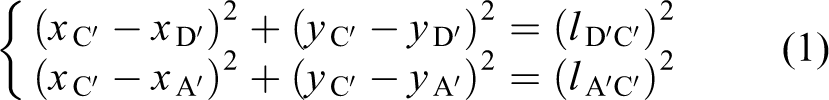
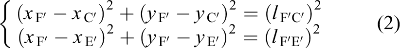
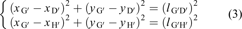
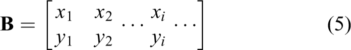
Therefore, all the coordinates for the points can be calculated. All the coordinates are then entered into matrix B

$B=\left[\begin{array}{cc}{x}_1& x_2\\ y_1& y_2\end{array}\cdots \begin{array}{c}{x}_i\\ y_i\end{array}\cdots \right]$

5

${\theta }_{\text{equal}}\text{=atan}\frac{0.5\left(y_{\text{max}}+y_{\text{max-1}}\right)}{0.5\left(x_{\text{max}}+x_{\text{max-1}}\right)}$

6

A kinematic simulation is performed in MATLAB [V7.12.0], with θ_equal as 0°, ±5°, and ±10°. The results are shown in Figure 7.

Figure 7.

Kinematic simulation result produced by MATLAB.

Based on the simulation results, this article can make a conclusion that the mechanism can change θ_equal from −10° to +10°. The range of θ_equal is big enough. ³³ Figure 7 also confirms that the design scheme can change its camber continuously with different initial inputs. This indicates that the design scheme can achieve the function of a camber morphing wing.

In order to improve the stiffness, several mechanisms will be connected by stringers as shown in Figure 8.

Figure 8.

Assemble diagram of the camber morphing wing model.

The aerodynamic characteristics of a wing are important for verifying the performance of a designed wing. This article selects a NACA64-0010 airfoil as the simulation model. Nodes for a normal airfoil are shown in Figure 9(a). In this study, the design scheme occupies 30% of the length of the airfoil. θ_equal is −5°, as shown in Figure 9(b).

Figure 9.

The outline of the airfoils: (a) outline of the NACA64-0010 and (b) outline of the camber morphing wing model.

The known conditions are presented in Table 1.

Table 1.

The known conditions for aerodynamic analysis.

V 0	50 m/s
α	5°
p	101,325 Pa
ρ	1.225 kg/m3
T	288 K
v	1.461 × 10−5 m2/s

V _o: the velocity of the oncoming airflow; α: the angle of attack; p: the pressure of the external environment; ρ: the air density; T: the air temperature; v: the viscosity of air.

In the flow field, the left part is a velocity inlet. The right part is a pressure outlet. The up and down lines are walls. The range of Y direction is from −10 m to 10 m. The range of X direction is from −10 m to 21 m. The flow field is shown in Figure 10(a).

Figure 10.

The model setting: (a) The flow field and (b) mesh of the morphing airfoil.

This article uses quadrilateral mesh. The local meshes around the airfoil are concentrated. For the leading edge, the size of the mesh is 0.01 m. For the trailing edge, the size of the mesh is 0.005 m. For the airfoil box, the size of the mesh is 0.02 m. The total number of nodes is 73,246 and the total number of quadrilateral cells is 72,720. The mesh model is shown in Figure 10(b).

A k − ε model, a stress coupled solver, the first order upwind, and stress-velocity couple algorithm are used in this article. When ${\theta }_{\text{equal}}\text{=}-5°$ , the results can be obtained as shown in Figure 11.

Figure 11.

Iteration curve of residuals with θ _equal = −5°.

In Figure 11, the iteration stops when the curves converge after 470 iterations. The lift coefficient (C _l) is 0.929 and the drag coefficient (C _d) is 0.081. C _l and C _d of the traditional airfoil are 0.5 and 0.0476, respectively. It is easy to see that the design scheme improves the C _l, which is increased by 85.8%. The lift-drag ratio is increased by 9.23%. X direction velocity and pressure contour are shown in Figure 12.

Figure 12.

Comparison results for the aerodynamic analysis: (a) X velocity contour of the morphing wing model, (b) X velocity contour of the traditional wing model, (c) pressure contour of the morphing wing model, and (d) pressure contour of the traditional wing model.

Figure 12(a) and (b) shows the X velocity contours of the morphing airfoil and the traditional airfoil. The flow velocity under the morphing trailing edge is slower than that under the traditional airfoil. The area of the slow flow in Figure 12(a) is larger than the area of the fast flow in Figure 12(b). Based on the basic law of motion of fluids, local pressure is low when flow is fast. So the pressure of the morphing airfoil is lower than that of the traditional wing, and the pressure differential is greater.

Therefore, this article can make a conclusion that the lift force of the morphing airfoil is greater than that of the traditional airfoil. The same conclusion can be obtained from Figure 12(c) and (d).

A comparative aerodynamic analysis is performed to explore the relationship between ${\theta }_{\text{equal}},\theta$ and C _l, C _d and lift-drag ratio. Five aerodynamic models are set up. They are camber morphing wings with the equivalent angles −1°, −2°, −3°, −4°, and −5°. The angles of attack range from 0° to 13°. The results are shown in the curve graphs in Figure 13.

Figure 13.

Aerodynamic analysis results: (a) the relationship between C _l and angles of attack, (b) the relationship between C _d and angles of attack, and (c) the relationship between the lift-drag ratio and angle of attack.

Figure 13(a) illustrates the relationship between C _l and the angle of attack α. When θ_equal doesn’t change, C _l increases and then decreases. When θ_equal changes from −1° to −5° and α doesn’t change, C _l increases. The most improvement of C _l is 85.8%. Figure 13(b) illustrates the relationship between C _d and α. When θ_equal doesn’t change, C _d always increases. When θ_equal changes from −1° to −5° and α doesn’t change, C _d increases. In Figure 13(c), when α increases, the curves for the five models first increase and then decrease. When θ_equal changes from −1° to −5°, the maximal lift-drag ratio increases and the angle of attack corresponding to the maximal lift-drag ratio decreases. The most improvement of lift-drag ratio is 9.23%.

Overall, this article can make a conclusion that the proposed camber morphing wing model can effectively improve aerodynamic characteristics by changing θ_equal, which will have great benefits for both civil and military applications.

Weighted adaptive AFS optimization algorithm with embedded Hooke–Jeeves search method

It is difficult to obtain the function expression for the nodes on the morphing trailing edge as they are calculated by nonlinear equations. So the optimization algorithm that uses function gradient is unsuitable for the proposed mechanism.

The swarm intelligent optimization algorithm can solve this problem. ³⁴ An AFS optimization algorithm, a typical algorithm of this type, can obtain the global optimal solution in the search field. ³⁵ The whole process of traditional AFS is shown in Figure 14. However, there is a disadvantage for traditional AFS. The range of vision and the length of the iteration step are constant, and the search method for prey action is random. ³⁶ A modified AFS optimization algorithm is proposed to overcome these limitations. The modified algorithm uses Hooke–Jeeves search method instead of random search method for prey action and uses weighted adaptive vision and adaptive iteration step length.

Figure 14.

The process of the traditional AFS optimization algorithm. AFS: artificial fish-swarm.

In the traditional AFS optimization algorithm, the current artificial fish is at the position X. Y is the food consistency of the current position X. “i” is non-negative integer. N is the total number of artificial fish. “gen” is the number of current generation. “MAXGEN” is the maximum of iteration generations. The range of vision is “visual.” The current direction is toward X_V. If the food consistency of X_V is bigger than that of X, it will take a step toward X_V, to the position X_next. Otherwise, it will go on searching within its range of vision. ³⁷ The process can be described by the following formulas.

$x_i^v=x_i+\text{visual\hspace{0.17em}}·r$

7

$X_{\text{next}}\text{=}\frac{X_V-X}{\Vert X_V-X\Vert }·\text{\hspace{0.17em}Step\hspace{0.17em}}·r$

8

r is a random number between −1 and 1.The process of the prey action, the swarm action, and the follow action are shown in Figure 15.

Figure 15.

The process of prey action, swarm action, and follow action: (a) swarm action, (b) follow action, and (c) prey action.

In Figure 15(a) and (b), the iteration depends on the prey action. X_i is the current position, X_j is the next position, δ is the crowding degree of the current position and “rand()” is a random number ranging from −1 to 1. “try_number” is the maximum of iterations of prey action. The prey action determines the velocity and efficiency of the whole algorithm. In Figure 15(c), the search method of the prey action is random that means the search is blind. The range of vision and the step length throughout the algorithm are constant. ³⁸ Although the velocity at the beginning is very fast, the convergence velocity at the end of the optimization is very slow, which requires a lot of initial fish and many iterations. ³⁹ To solve this problem, this article proposes a weighted adaptive vision that uses the farthest position X_farthest and the current optimal position X_{currentoptimal} where the food consistency is highest. Figure 16 shows the process for setting the vision for each generation.

Figure 16.

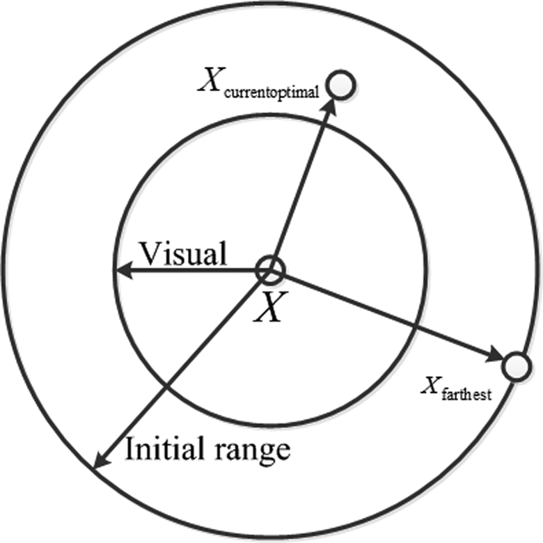
Adaptive vision and step.

This modified method calculates the position of the farthest fish among all the initial fish and the position of the current optimal fish. The optimal solution to the problem may appear in the direction of $X_{\text{farthest}},X_{\text{currentoptimal}}$ , or neither. The vision of the current generation is set by the following formulas

$V^i=\alpha ·\text{dist}\hspace{0.17em}(X^i,X_{\text{farthest}}^i)+(1-\alpha )·\hspace{0.17em}dist(X^i,X_{\text{currentoptimal}}^i)$

9

${\text{Step}}^i=\text{rand}()·V^i$

10

α is a weighted coefficient between 0 and 1. The value of α can be changed to adjust the vision. The range of vision will adaptively change based on the different X_farthest and X_{currentoptimal}. The length of the iteration step will also adaptively change after a change in the vision.

The search method for the prey action is random, which makes the search sightless and inefficient. All the search results depend on the total number of artificial fish. ⁴⁰ If users want to get the final result fast, there must be a large number of artificial fish. Therefore, the high-efficiency Hooke–Jeeves search method is embedded in the prey action instead of the random search method. The Hooke–Jeeves search method can search the local optimal solution. It is not sightless and pointed. It can efficiently improve the velocity of convergence. The codes for the modified prey action are shown in Table A1 in the appendix.

To verify the performance of the modified AFS optimization algorithm, multi-peak-value functions are used for the optimization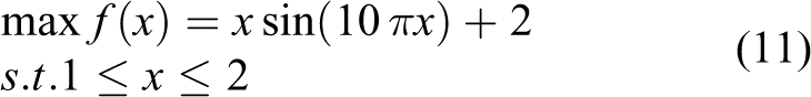

$\begin{array}{l}\max f\left(x\right)=x\text{sin}(10\text{π}x)+2\\ s.t.1\le x\le 2\end{array}$

11

$\begin{array}{l}\max f(x)=\frac{\text{sin}\sqrt{x^2+y^2}}{\sqrt{x^2+y^2}}+{\text{e}}^{\frac{\text{cos}2\pi x+\text{cos}2\pi y}{2}}-2.71289\\ s.t.x\in [-1,1],y\in [-1,1]\end{array}$

12

The functional images are shown in Figure 17.

Figure 17.

Function images: (a) function with one variable and (b) function with two variables.

Figure 17 shows that the function has many local peaks that have a strong effect on the optimization algorithm. The two functions are used to verify the modified AFS algorithm. First, the traditional AFS algorithm and the modified AFS algorithm are used to calculate the maximum of equation (11). The results are shown in Figure 18.

Figure 18.

Results of the optimization for the function with one variable: (a) Iteration process of the traditional AFS algorithm, (b) iteration process of the modified AFS algorithm, (c) optimal solution for different generations of the traditional AFS algorithm, and (d) optimal solution for different generations of the modified AFS algorithm. AFS: artificial fish-swarm.

In the traditional AFS algorithm, there are 50 initial artificial fish and the maximal generation is 50. In the modified AFS algorithm, there are only 10 initial artificial fish and the maximal generation is 10. In Figure 18(a), the curve converges at step 37 using the traditional AFS algorithm. In Figure 18(b), the curve converges at step 3 using the modified AFS algorithm. The results of the binary function are shown in Figure 19.

Figure 19.

Results of the optimization for the binary function: (a) Iteration process of the traditional AFS algorithm, (b) iteration process of the modified AFS algorithm, (c) optimal solution for different generations of the traditional AFS algorithm, and (d) optimal solution for different generations of the modified AFS algorithm. AFS: artificial fish-swarm.

In the traditional AFS algorithm, there are 300 initial artificial fish and the maximal generation is 150. However, in the modified AFS algorithm, there are only 20 initial artificial fish and the maximal generation is 20. In Figure 19(a), the curve converges at step 53 using the traditional AFS algorithm. In Figure 19(b), the curve converges at step 11 using the modified AFS algorithm. This article also uses MATLAB optimization box GUI to do comparison. The solving algorithm is GA. The number of generation is 100 and the number of population is 2000. The final result is the same as the result obtained by the modified AFS. The execution time of MATLAB optimization box is 9.73246 s, while the time of the modified AFS is 5.00137 s.

Based on the earlier results, this article can make a conclusion that the modified AFS optimization algorithm performs better than the traditional AFS optimization algorithm; it requires fewer artificial fish and iteration generations.

In order to make a further test, this article makes a comparison with another algorithm. The selected algorithm is PSO. The test function is function (12). For PSO, the number of particle is 100, the number of each particle dimensions is 2, and the number of iteration generations is 300. For the modified AFS, the number of artificial fish is 20 and the number of iteration generations is 20. The total number of tests for each algorithm is 10. The optimal solution of the second example is 1.0054. The final results are for PSO, the times of obtaining global optimal solution are 6 as shown in Figure 20(a) to (f). For the modified AFS, the times of obtaining global optimal solution are 9 as shown in Figure 21(a) to (i). Therefore, the modified AFS has more powerful ability on searching the global optimal solution with less number of population quantity and less number of iteration generations. The robustness of the modified AFS is better.

Figure 20.

Ten results of iteration for PSO. PSO: particle swarm optimization.

Figure 21.

Ten results of iteration for the modified AFS. AFS: artificial fish-swarm.

This article also does comparison with an exact algorithm. Both AFS and PSO are stochastic algorithm. ⁴¹ In order to make the article comprehensive, this article selects an exact algorithm that is the filled function method to do comparison. ⁴¹ The detailed introduction of this method is provided in the literature. ⁴² It has been proved that it is a valid optimization algorithm for global optimization. ⁴³ This article also does 10 optimizations by this method for the second example. The solutions and the execution time are shown in Table B1 in the appendix.

From the results, this article can conclude that the filled function method can obtain the optimal solution of the second example. But it needs more iteration steps and wastes more time. It is very sensitive about the initial values. If the initial values are not fit, the iteration steps and execution time will be very large. There is a limitation for this method that needs to know the expression of all the functions for the reason, which will use their derivatives. Therefore, if there are many nonlinear equations in the optimization and can’t obtain their expressions, this method does not fit. However, the modified AFS doesn’t need the expression of all the function as introduced in the last part of the introduction in this article. It is not sensitive about the parameters and very robust. It need less number of iteration steps and less number of artificial fish. When increasing the number of iteration generations and the number of artificial fish, the solution accuracy will be higher. It is more convenient and more intelligent.

Therefore, the proposed algorithm is used to optimize the mechanism. The lengths of the slanted bars FC and JH strongly affect the camber of the morphing trailing edge, as shown in Figure 6(a); therefore, the lengths of FC and JH are optimized in this study.

There is an important line, that is, the median line of the trailing edge. This line will pass the middle points of AB, CD, GH, and KL. Studies on morphing trailing edges consider three kinds of median lines when testing the bending degree: a cantilever beam curve, a circular curve, and an inverse cantilever beam curve. The functions of the three curves are as follows ⁴

$f_s(x)=\frac{\Delta z}{2}(3\frac{x^2}{c_{WL}^2}-\frac{x^3}{c_{WL}^3})$

13

$f_s(x)=\frac{1}{2}(\Delta z+\frac{c_{WL}^2}{\Delta z})-\sqrt{\frac{1}{4}{(\Delta z+\frac{c_{WL}^2}{\Delta z})}^2-x^2}$

14

$f_s(x)=\frac{\Delta z}{3}(\frac{x^2}{c_{WL}^2}+2\frac{x^3}{c_{WL}^3})$

15

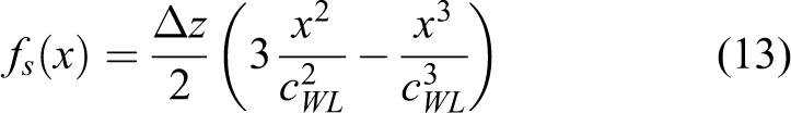
Δ_z is the vertical deformation distance of the end of the morphing trailing edge and c_WL is the chord length of morphing trailing edge.

If the median curve of the proposed mechanism fits the function curves above, the mechanism is satisfactory. ⁴ The function curves are shown in Figure 22 when Δ_z is 9 and c_WL is 100.

Figure 22.

Function curves.

In Figure 22, the circular curve is between the cantilever beam curve and the inverse cantilever beam curve, so this article selects the circular curve as the fitting objective. The aim is to make the fitting error for the circular curve and the median curve of the design scheme as small as possible. Therefore, the objective function is

$\min {\displaystyle \sum \sqrt{y{z}_i^2-y\_{\text{circle}}_i^2}}$

16

$\begin{array}{l}s.t.11\le l_{\text{FC}}\le 15\\ 11\le l_{\text{JH}}\le 15\end{array}$

y_zi – – is the vertical coordinate of the ith point on the median curve of the mechanism and $y\_{\text{circle}}_i$ – – is the vertical coordinate of the ith point on the circular curve.

The weighted adaptive AFS optimization algorithm with the embedded Hooke–Jeeves search method is then applied to optimize the problem. The optimization results are shown in Figure 23.

Figure 23.

Optimization results of the design scheme: (a) Iteration process of the modified AFS algorithm and (b) optimal solution for different generations of the modified AFS algorithm. AFS: artificial fish-swarm.

The optimization uses 20 artificial fish and 30 iteration generations. It costs 47.34957 s. This article also tries to do optimization using the traditional AFS algorithm by 20 artificial fish and 30 iteration generations. But it can’t get correct global solution in the given area. Then this article uses the traditional AFS algorithm by 300 artificial fish and 150 iteration generations. The correct solution can be obtained by costing 90.022699 s.

From Figure 23(a), the iteration converges at step 4. The optimal solution is FC = 11 cm, JH = 14.6135 cm. The initial length of both FC and JH is 9.1426 cm before the optimization. The initial fitting error is 1.8272, and the optimization reduces it to 0.2152. The effect of the optimization is obvious. The fitting graphs before and after the optimization are shown in Figure 24.

Figure 24.

Fitting graphs before and after the optimization: (a) before the optimization and (b) after the optimization.

Comparing Figure 24(a) with Figure 24(b), it is clear that the optimized model fits the circular curves more accurately. The optimized model data are input into FLUENT [version 6.3] to perform the aerodynamic simulation. When θ_equal is −5° and α is 5°, C _l is 0.85, C _d is 0.073, and the lift-drag ratio is 11.64. Before the optimization, C _l is 0.929, C _d is 0.081, and the lift-drag ratio is 11.469. Therefore, the optimization decreases C _l and C _d by 8.5% and 9.88% and increases the lift-drag ratio by 1.5%.

The results indicate that the airplane can achieve higher aerodynamic efficiency by lower C _l and C _d. The results also indicate that the optimized model can achieve a higher maximal lift-drag ratio. Therefore, the optimization effectively improves the design scheme.

Conclusion

This article proposes a camber morphing wing model. A mathematical model is set up and a kinematic simulation is performed to verify the kinematic performance. The kinematic results indicate that the kinematic performance is satisfactory. An aerodynamic model is set up and some aerodynamic analysis has been done. The results indicate that the design scheme can effectively improve the aerodynamic performance by changing the camber of the wing. This article proposes a modified optimization algorithm called the weighted adaptive AFS optimization algorithm with embedded Hooke–Jeeves search method. Calculation of the maximum unitary function and binary function verifies that the performance of this algorithm is excellent. It needs fewer artificial fish and iteration generations. It occupies less computer resources. The proposed algorithm can effectively improve the convergence velocity and obtain the accurate global solution. It is more robust by the comparison of test results among PSO, the filled function method, and the modified AFS. Finally, the mechanism is optimized, which significantly decreases the fitting error and improves the aerodynamic characteristics. Based on the optimization results, this article make a conclusion that the optimized mechanism can provide better aerodynamic shape that can provide better aerodynamic characteristics. For future work, the prototype is under manufacture. Some practical tests and verification will be done, such as kinematic experiments, aerodynamic experiments, and control experiments.