Planning with ants

Abstract

Rapidly exploring random trees (RRTs) have been proven to be efficient for planning in environments populated with obstacles. These methods perform a uniform sampling of the state space, which is needed to guarantee the algorithm’s completeness but does not necessarily lead to the most efficient solution. In previous works it has been shown that the use of heuristics to modify the sampling strategy could incur an improvement in the algorithm performance. However, these heuristics only apply to solve the shortest path-planning problem. Here we propose a framework that allows us to incorporate arbitrary heuristics to modify the sampling strategy according to the user requirements. This framework is based on ‘learning from experience’. Specifically, we introduce a utility function that takes the contribution of the samples to the tree construction into account; sampling at locations of increased utility then becomes more frequent. The idea is realized by introducing an ant colony optimization concept in the RRT/RRT* algorithm and defining a novel utility function that permits trading off exploitation versus exploration of the state space. We also extend the algorithm to allow an anytime implementation. The scheme is validated with three scenarios: one populated with multiple rectangular obstacles, one consisting of a single narrow passage and a maze-like environment. We evaluate its performance in terms of the cost and time to find the first path, and in terms of the evolution of the path quality with the number of iterations. It is shown that the proposed algorithm greatly outperforms state-of-the-art RRT and RRT* algorithms.

Introduction

The optimal path-planning problem, which can be formulated as the task of driving a robot from an initial state x _A to a goal state x _B with the minimum cost, is one of the most fundamental problems in robotics. Despite a vast literature, it is still a challenging problem in many situations. Furthermore, in safety-of-life applications, such as search-and-rescue missions, or disaster relief, we aim to find the best possible path in a given time. Sampling-based methods, such as rapidly exploring random trees (RRTs), ¹ are widely used to solve this problem, since the method offers low computational complexity and is efficient in finding a solution. However, the performance of the method can be increased by modifying the way in which the state space is sampled. Rapidly exploring random trees typically perform a uniform sampling of the state space. The uniform sampling treats all samples equally; instead, new samples can be picked at locations where some utility function is optimized. Thus, we aim to sample at locations with a high utility; this utility function is constructed so as to either optimize a time to find a feasible solution, or to improve an already found solution.

Thus, our goal in this work is to answer the question of how to sample to optimize the selected utility function. Furthermore, the definition of the utility function allows us to formulate a framework that is able to incorporate heuristics that will guide the sampling strategy according to the user requirements. This would enable us to extend the original RRT* algorithm ² to informative path-planning and exploration applications in unknown environments, where our goal is to sample more often where there is more information, or to employ the user’s prior knowledge to perform a more intelligent sampling that optimizes some predefined criteria, for instance, avoiding harsh terrains in search and rescue missions. This could easily be introduced into our utility function. However, in this work, we focus on the shortest path-planning problem and formulate a utility function that optimizes the path cost with respect to distance. We suggest further extensions of the algorithm in the concluding discussion of possibilities for future work.

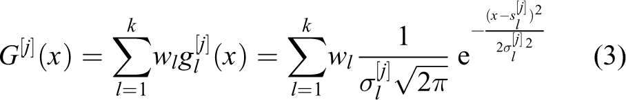
Inspired by machine-learning techniques, we augment our sampling strategy by taking the already accumulated samples into account. This can be interpreted as continuous learning of the probability density function, which represents the optimal sampling distribution at each moment and sampling according to it. To determine the optimal sampling distribution, we rely on ant colony optimization (ACO) for continuous domains (ACOℝ). We chose ACOℝ because it offers superior performance compared with both Monte-Carlo methods and other swarm optimization techniques. ³ The ACOℝ algorithm distributes virtual ants according to a utility function that evaluates the ants’ relevance and so determines the sampling distribution (as illustrated in Figure 1). The utility function is constructed to trade exploitation of the state space, that is, optimization of the constructed tree, and exploration of the state space, which favours a growth of the tree in as yet explored regions of the state space. Given the tree we have constructed so far, we analyze: (i) how much the sample exploits the current solution; (ii) how much a sample contributes to exploration of the state space. Based on that, we update our ants, which will modify the sampling distribution and, in consequence, the way we construct our tree to solve the path-planning problem.

Figure 1.

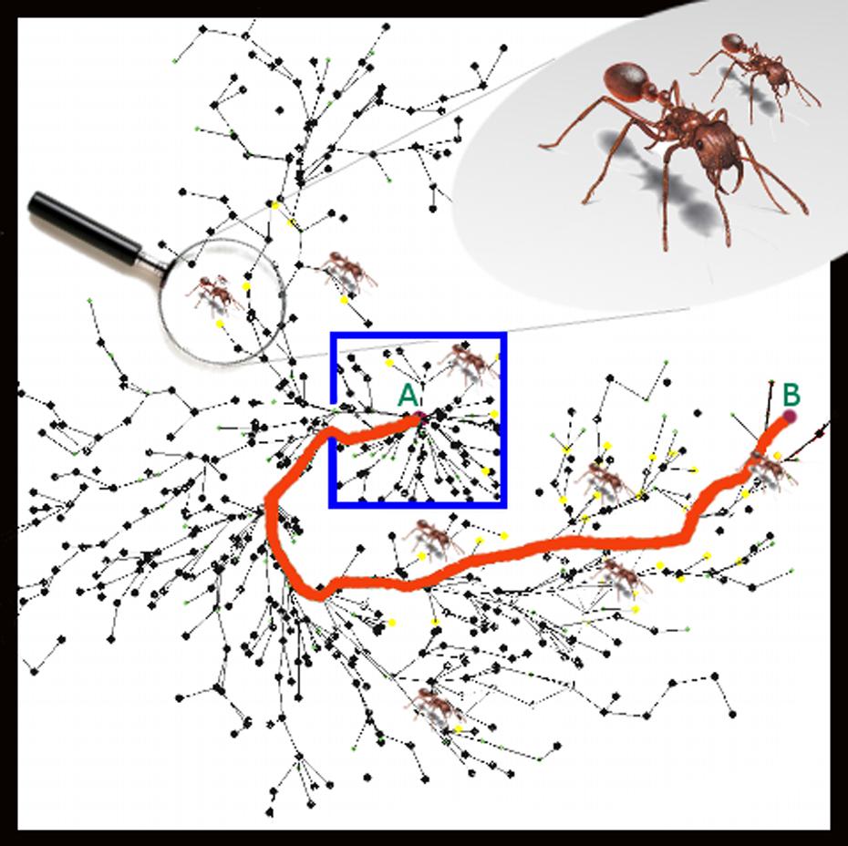
Example of one path generated with the proposed ACO-RRT* algorithm. We build a rapidly exploring random tree based on a modified sampling strategy that learns from previous experience.

Related work

Sampling-based path-planning algorithms are widely used because of their efficiency in providing path-planning solutions in high-dimensional spaces. These methods are well exemplified by probabilistic roadmaps (PRMs) ⁴ and rapidly exploring random trees (RRTs); ¹ a modification of the RRT algorithm, called RRT*, is also known to achieve asymptotic optimality with respect to a given cost function. ²

In recent years, a great amount of sampling-based path-planning algorithms have been proposed. ^{5 –11} These works have in common that they outperform the RRT* algorithm by modifying and optimizing some of the subroutines that compose the original RRT* algorithm. However, the cited algorithms are specifically designed to solve the optimal shortest path-planning problem under certain restrictions. Here, we aim to go one step further and propose a framework that allows us to introduce some heuristics into the original RRT and RRT* algorithms. These heuristics are incorporated into the algorithm by modifying the sampling distribution, which is learnt online according to those heuristics as we sample the state space. The advantage of defining such heuristics is twofold: (i) it enables the introduction of some additional knowledge to solve the path-planning problem more efficiently; (ii) it could be used in conjunction with any of the aforementioned works to improve their performance. Specifically, in this work we will show that our approach, combined with shortest path heuristics, outperforms the state-of-the-art RRT and RRT* algorithms.

Sampling-based path planners consist of several subroutines that can be optimized individually to improve the algorithm’s performance, which also make the methods very attractive. Denny et al. proposed a ‘lazy planning’ to improve the collision checking by the assumption that only 10% of the collisions checks are positive. ¹² Conversely, algorithms like RRT connect ¹³ and the one proposed by Urmson and Simmons ¹⁴ increases the algorithm performance by heuristically biasing the tree growth. This tree growth has also been adapted by Denny et al., ¹⁵ who adapted the branch size according to the space in heterogeneous environments. In contrast to previous works, here we focus on a modification of the sampling strategy. Essentially, if we can identify regions of higher importance, that is, regions in the state space that could help us to improve our current path, then we should sample these regions more often.

It is possible to dichotomize sampling strategies for path planning into importance sampling and adaptive sampling. Importance sampling methods exploit some predefined a-priori sampling strategy. Examples include goal-biased sampling, ¹⁶ medial-axis sampling, ¹⁷ where samples are taken from the medial axis of free space, and the bridge test, ¹⁸ which is designed to solve narrow passage problems. These methods are specifically designed to solve concrete problems. Alternatively, in adaptive sampling methods, the samples are drawn from a distribution that is adapted based on the information obtained from previous samples, which makes them more flexible. Siméon et al. propose the visibility PRM algorithm, ¹⁹ which just takes samples from the unexplored area within the planner visibility region. Although the constructed roadmaps are significantly smaller, the computation of the visibility region is expensive. Adaptive dynamic domain RRT adapts the previous concept to the RRT algorithm. ²⁰ In this work, we additionally consider the importance of the previous samples, which are not necessarily within the visibility region. This is exploited for PRMs through an utility-guided sampling by Burns and Brock. ²¹ There, the authors do not aim to learn the sampling distribution, but to perform a Monte-Carlo sampling and select the samples with a higher utility. However, our focus lies in rapidly exploring random trees, owing to their efficiency, since they do not require any pre-computation time, as in PRMs. Adaptive sampling within the RRTs framework has also been exploited in recent works. ^{22 –25} In contrast to our algorithm, these are able neither to incorporate nor to learn arbitrary heuristics.

The work of Rickert et al. ²⁶ inspires the definition of our utility function. In their work, Rickert et al. propose the exploring-exploiting tree algorithm, which balances exploitation and exploration to construct the tree more effectively. Yet this method requires some environment-dependent pre-computing time to grow the tree, which does not make it suitable for online planning. The exploration-exploitation trade-off has also been employed in several works. ^{27 –29} Alterovitz et al. ²⁸ propose the rapidly exploring roadmaps algorithm. This algorithm first finds a solution, as in RRTs, and then refines this solution. Balancing exploration and exploitation is also employed by Persson and Sharf, ²⁹ who generalize the A* algorithm to allow sampling-based motion planning. Also Akgun and Stilman ²⁷ have developed an algorithm that trades off exploration and exploitation to improve the RRT* in high dimensions. This is done by introducing sampling heuristics. Our algorithm is also based on sampling heuristics, which are learnt using machine learning. In contrast to the aforementioned studies, ^{27 –29} our framework allows us to introduce sampling heuristics that are not just specifically designed for the optimal shortest path planning but also for different applications.

Our goal in this paper is not just to define a framework that can incorporate arbitrary heuristics. In addition, we aim to learn the sampling distribution of the planning algorithm that better fits the user-defined heuristics. This is done by introducing machine-learning techniques. Morales et al. ³⁰ divide the planning problem into several subproblems, and then employ machine learning to select a roadmap from a set that is more adequate to solve each of the subproblems. In the last step, the selected roadmaps are fused to obtain a global one. Machine learning is also introduced by Diankov and Kuffner ³¹ into A* to select the best heuristic from a set in order to improve the algorithm performance. Both of these algorithms ^30,31 require a discrete predefined set from which they select the best roadmap or heuristic, respectively. In contrast, we aim to apply machine learning to learn not a discrete set but a continuous distribution.

This paper is strongly influenced by the idea of cross-entropy motion planning outlined by Kobilarov. ³² Here, Kobilarov ³² learns the sampling distribution from previous samples by evaluating its entropy. Its limitation comes from the high computational requirement to calculate the sampling distribution for the environment, which does not make it feasible for real-time applications. We improve this concept by using an ant colony optimization algorithm to learn the sampling distribution. ³ Ant colony optimization has also been used, by Mohamad et al., ³³ in the context of PRMs. The goal of Mohamad et al. ³³ was to reduce the number of intermediate configurations from an initial to a goal position. Although it has a different objective, that work serves as an inspiration to incorporate the ACO into a sampling-based path planner. Learning the sampling distribution, together with the definition of a novel utility function, lets us derive a scalable algorithm suitable for real-time path-planning applications.

In the remainder of this paper, we briefly describe the rapidly exploring random trees and ant colony optimization algorithms that serve as the basis of our work. We then introduce the proposed algorithm and extend it to allow an anytime implementation. We evaluate and discuss the algorithm performance and finally draw conclusions and discuss avenues for future work.

Background

Rapidly exploring random trees

The rapidly exploring random trees (RRTs) algorithm is a solution to the path planning problem in complex high-dimensional spaces. ¹ The RRT algorithm iteratively constructs a graph $\mathcal{G}(\mathcal{V},\mathcal{E})$ (tree) with a set of vertices ν and edges Ε, with the goal of establishing a path between x _A and x _B in the state space – a feasible trajectory ${\mathcal{T}}_{A,B}(\mathcal{G})$ . The key steps of the RRT algorithm are summarized in Algorithm 1.

The algorithm is realized as follows. We draw a sample x_rand randomly from a uniform distribution defined over free space using the function SampleFree. Then the Nearest function finds the nearest neighbour (in terms of the cost-to-reach) of x_rand from the set of vertices ν. We use the function Steer to simulate driving the robot from x_nearest to x_rand according to our controller. We drive the robot a maximum distance η. This is a user-selected parameter, which sets the maximum branch size. As the output we obtain the state x_new. If the trajectory $\mathcal{T}(x_{\text{nearest}},x_{\text{new}})$ does not collide with any obstacles, we add the vertex x_new and the edge $\mathcal{T}(x_{\text{nearest}},x_{\text{new}})$ to the tree G. Given the current tree, we search the best path ${\mathcal{T}}_{A,B}(\mathcal{G})$ from x _A to x _B using the function FindBestPath. If there is no feasible path, the output would be a void set. We repeat this process during n iterations.

The RRT* algorithm is an evolution of the RRT algorithm, which has been shown to be asymptotically optimal. ² We describe the RRT* in Algorithm 2. It differs from RRT in two aspects: choosing a parent and rewiring. In contrast to RRT, we choose the parent of x_new as the node from the set X_near that allows us to reach x_new with the minimum cost. X_near is calculated using the function Near, which is defined as

$\mathtt{N}\mathtt{e}\mathtt{a}\mathtt{r}(x,\mathcal{V}):=\left\{\parallel x-x\text{'}\parallel \le \mathit{r}(\text{card}(\mathcal{V}))\right\}$

1

with

$r(\text{card}(\mathcal{V}))=\min \{\gamma {(\log (\text{card}(\mathcal{V}))/\text{card}(\mathcal{V}))}^{1/d},\eta \}$

2

where $\text{card}(\mathcal{V})$ is the number of elements in set ν, γ is a constant and d is the number of dimensions of the state space. The RRT* algorithm also incorporates a rewiring process to find an optimal trajectory. This is done by finding minimum cost sub-paths. Here, we define two different costs: $\mathtt{\text{Cost}}(x,\mathcal{G})$ is the cost-to-reach sample x from x _A following the tree G. $\mathtt{\text{Cost}}(\mathcal{T}(x,x\text{'}))$ would be the cost of going directly from x to x', regardless of the obstacles. In this work, we define the cost between two samples $\mathtt{\text{Cost}}(\mathcal{T}(x,x\text{'}))$ as the Euclidean distance between them. The cost $\mathtt{\text{Cost}}(x,\mathcal{G})$ is the sum of these Euclidean distances along the edges towards x.

Ant colony optimization for continuous domains

Ant colony optimization is a nature-inspired algorithm to solve hard combinatorial optimization problems. ³⁴ Its driving principle comes from the behaviour of ants when searching for food. First, they leave the nest walking in random directions. Once they find a food source, they come back to the nest, leaving a pheromone trail on the ground. The pheromone deposited depends on the quality and quantity of the food and guides the other ants to the food source. Based on the same principle, ant colony optimization for continuous domains (ACOℝ) is proposed to solve continuous optimization problems. ³ This work inspires our sampling strategy, in which the ants, according to their utility, will decide where to sample next.

The ants are stored in a table T, as depicted in Figure 2. Each row contains one of the k ants, where $s_l=[s_l^{[1]},s_l^{[2]}\mathrm{,}\dots ,s_l^{[d]}]$ is the vector of coordinates describing the lth ant’s location and d is the number of dimensions of the state space. The ant’s utility is given by u_l, which determines the importance of the lth ant. The utility is defined according to the algorithm’s optimization objective.

Figure 2.

T-table of the ACOℝ algorithm. It stores the k ants, sorted according to their utility given by the elements of u. Together with the ants’ coordinates, the elements of w determine the probability density function described by the ants.

The algorithm works as follows. First, we take a sample $x_{\text{rand}}=[x_{\text{rand}}^{[1]}\mathrm{,...},x_{\text{rand}}^{[j]}\mathrm{,...},x_{\text{rand}}^{[d]}]$ , where each of the components $x_{\text{rand}}^{[j]}$ is drawn from a Gaussian kernel probability density function

$G^{[j]}(x)={\displaystyle \sum _{l=1}^k}{w}_l{g}_l^{[j]}(x)={\displaystyle \sum _{l=1}^k}{w}_l\frac{1}{{\sigma }_l^{[j]}\sqrt{2\pi }}{\text{e}}^{-\frac{{(x-s_l^{[j]})}^2}{2{\sigma }_l^{[j]}{}^2}}$

3

with $j=1,2,\mathrm{...},d,\text{ and }{\sigma }_l^{[j]}$ the lth ant’s standard deviation in dimension j. The standard deviation is calculated as the average distance from the lth ant to the rest of the ants stored in T

${\sigma }_l^{[j]}=\xi {\displaystyle \sum _{e=1}^k}\frac{|s_e^{[j]}-s_l^{[j]}|}{k-1}$

4

where ξ > 0 is the pheromone evaporation rate, which avoids the algorithm converging too quickly before approaching the optimal solution. The parameter w_l from w is set as

$w_l=\frac{1}{qk\sqrt{2\pi }}{\text{e}}^{-\frac{{(l-1)}^2}{2q^2{k}^2}}$

5

where q is a user-defined parameter. When q is small, the best ranked solutions are strongly preferred. The vector of weights w is normalized so that the integral of the probability density function $G^{[j]}(x)$ over the entire space is equal to one. The value of w_l is initialized and is not modified during the execution of the algorithm.

Next, we sort the table T in descending order according to the utility given by vector u and insert the new sample x_rand. The sample x_rand will now become an ant. In this way, samples with a higher utility will move up the table and will be selected with a higher probability. If the sample’s utility is higher than the last ranked solution s _k , this last one will be removed from the table T to keep k ants in the algorithm. This loop goes on during n iterations.

ACO-RRT* algorithm

In this work, we propose the ACO-RRT* algorithm, which aims to improve on the RRT and RRT* performance by modifying the sampling distribution using ant colony optimization for continuous domains. Our motivation lies in learning from the experience. This means that, after sampling, we evaluate how much that sample contributed to improve our current path. This evaluation will influence how we obtain the next sample.

The algorithm consists of five steps (see Figure 3). First, we initialize the ants that will generate future samples. Second, we sample from the distribution described by the current ants. Then we update our tree according to the original RRT/RRT* algorithm. After that, we calculate the utility of that sample based on how much it could improve the current path. This is divided into two factors: (i) exploitation of the current solution and (ii) exploration of the state space to find a new, better solution. Based on that utility, we update the ants and resample according to the new distribution. The algorithm is formulated in Algorithms 3, 4 and 5, and is described in detail in the following subsections.

Figure 3.

ACO-RRT* algorithm block diagram. Each of the five blocks points to its respective lines from Algorithm 4.

Initialize ants

The first part of the algorithm consists of filling the table T with k ants (see Algorithm 3). We take a sample from a uniform distribution defined over the obstacle-free space (line 2). Then we insert its position coordinates in row l, where $x_{\text{rand}}^{[j]}$ represents the coordinate of x_rand at the jth dimension (lines 3 and 4). We initialize the utility u_l to zero. To calculate the utility, we require the exploitation and exploration utility as well as the α that trades off the two factors. These three elements ( ${\mathcal{F}}_l\mathrm{.}{U}_{\text{exploit}},{\mathcal{F}}_l\mathrm{.}{U}_{\text{explore}},{\mathcal{F}}_l\mathrm{.}\alpha$ ) are stored in set ℱ _l and initialized to zero. (The notation A.b makes reference to the element b that is part of set A.) The parameter w_l is computed according to equation (5) (lines 5 and 6). This initialization is only performed once, at the beginning of the algorithm.

Sample ACO

Given the table T, we sample from the probability density function described by the ants (line 4 in Algorithm 4). The following method is equivalent to sampling directly from the distribution described by equation (3). First we select an ant l with a probability

$p_l=\frac{w_l}{{\displaystyle \sum _{e=1}^k}{w}_e}$

6

with w_e given by equation (5) and $l=1,2,\mathrm{...},k$ . The new sample will be $x_{\text{rand}}=[x_{\text{rand}}^{[1]}\mathrm{,...},x_{\text{rand}}^{[j]}\mathrm{,...},x_{\text{rand}}^{[d]}]$ . The position coordinate $x_{\text{rand}}^{[j]}$ is taken from a Gaussian distribution with $x_{\text{rand}}^{[j]}~\mathcal{N}(s_l^{[j]},{\sigma }_l^{[j]}{}^2)$ . This function outputs the new sample x_rand, as well as the ant index l that generated it. We use rejection sampling to select a sample that belongs to the free space.

This modification of the sampling strategy implies that the algorithm cannot guarantee the theoretical asymptotic optimality from RRT*. However, simulation results suggest that the proposed algorithm is able to approach the optimal solution. The explanation for such behaviour lies in the fact that the ants are associated with Gaussian probability density functions. Samples extracted from such a function can take values from an infinite domain that results in sampling over the complete state space. Even in the worst case, when all ants could converge to a single point, the variance of the distributions associated with the ants will be always slightly greater than zero. This fact guarantees that the state space will always be fully sampled and, therefore, the algorithm will approach the optimal solution.

Construct tree

The next step is to construct the tree according to the basic rapidly exploring random tree path planner. This step corresponds to lines 4–8 in Algorithm 1 (RRT) and lines 4–23 in Algorithm 2 (RRT*). This function needs the x_rand sample and the current tree. The output of this function is the new vertex x_new added to the tree as well as the new constructed tree G. Based on the new sample and the current tree, we calculate the utility function that will modify how the ants sample the states’ space.

Calculate utility

The key part of the algorithm is the calculation of the utility of the x_new sample. It corresponds to lines 6–18 in Algorithm 4. We define the utility function as a trade-off between exploitation and exploration. Exploitation (i) tries to go directly to the goal position using the shortest possible path, if no path has been found, and, (ii) once a path has been found, tries to improve it. Exploration aims to sample at those locations have not yet been sampled. It helps us to: (i) find a first path by exploring the state space and (ii) search for new better paths once we have found a solution. The utility function $U(x,\mathcal{G})$ of sample x given the tree G is defined as

$U(x,\mathcal{G})=\alpha \cdot U_{\text{exploit}}(x,\mathcal{G})+(1-\alpha )\cdot U_{\text{explore}}(x,\mathcal{G})$

7

where α models the trade-off between exploitation and exploration, $U_{\text{exploit}}(x,\mathcal{G})$ is the exploitation utility, and $U_{\text{explore}}(x,\mathcal{G})$ is the exploration utility.

Exploration utility

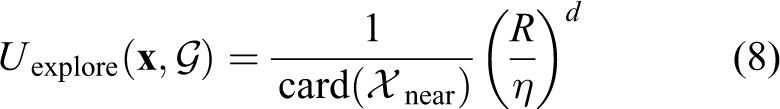
The exploration utility $U_{\text{explore}}(x,\mathcal{G})$ represents the density of samples in the tree G in the vicinity of sample x and is defined as

$U_{\text{explore}}(x,\mathcal{G})=\frac{1}{\text{card}({\mathcal{X}}_{\text{near}})}{\left(\frac{R}{\eta }\right)}^d$

8

with ${\mathcal{X}}_{\text{near}}\leftarrow \mathtt{\text{Near}}(x,\mathcal{V})$ the set of neighbours of x given by equation (1), $\text{card}({\mathcal{X}}_{\text{near}})$ the number of elements in the set X_near, η a parameter of the RRT/RRT* path planner and R the connection radius. We define $R=r(\text{card}(\mathcal{V}))$ for RRT* with $r(\cdot )$ given by equation (2), and $R=\eta$ for RRT.

The first term of the product models a decay of the exploration utility as proportional with respect to the number of elements in X_near. That implies that a sample that has a low number of neighbours in the current tree G will have a high exploration utility. Therefore, the exploration utility function will bias the exploration towards the not-yet-sampled state space. However, the number of neighbours of a sample depends on the connection radius R given by the RRT/RRT* algorithm. The bigger the connection radius, the higher the probability of having a larger number of neighbours. As the tree growths, the connection radius decreases. To make the exploration utility independent of the tree’s current state, we introduce a second term ${\left(R/\eta \right)}^d$ to act as a normalization factor.

Exploitation utility

The exploitation utility takes advantage of the acquired knowledge about the state space. Here, we distinguish two modes: no path found and path found, so that we can incorporate the information about the current solution. To add more flexibility to the algorithm, we assign to it the parameter α, which trades off exploitation and exploration in equation (7), one of the two possible values: (a) $\alpha =\widehat{\alpha }$ if no path was found; (b) $\alpha =\stackrel{⌣}{\alpha }$ otherwise.

No path found

Before finding a first path, we bias the sampling to connect the state x with the goal as quickly as possible regardless the obstacles. ¹⁶ Conversely, the exploration utility will bias the growth to obtain a path free of collisions. In this mode, we define the exploitation utility as

${\widehat{U}}_{\text{exploit}}(x,\mathcal{G})=1-\frac{\mathtt{\text{Cost}}(\mathcal{T}(x,x_B))}{c_{\text{max}}}$

9

where the cost to go directly to the goal from x, $\mathtt{\text{Cost}}(\mathcal{T}(x,x_B))$ , is normalized by the maximum cost c_max to reach the goal from any of the possible states. We can observe that sampling in the goal state will have the maximum utility since it will direct the tree growth towards the goal position.

Path found

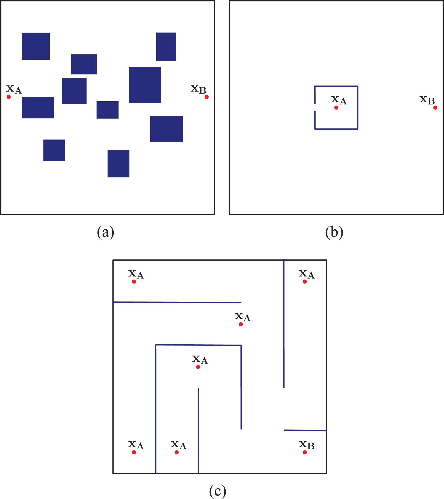
Once we have found a path, we can exploit this information to derive a richer exploitation utility function. We consider two possible situations: path improvement (see Figure 4(a)), and no path improvement (see Figure 4(b)).

Figure 4.

Graphical representation of the exploitation utility in the path found mode: (a) path improvement; (b) no path improvement. The black square represents an obstacle. The red dot corresponds to the sample x. The black lines and green dots represent the current tree G. The superposed thick blue line is the best found path before sampling the state x. The dashed yellow line is the new best path after sampling x. Arrows represent the direct path between one state and the goal x _B .

Consider that sample x leads to an improvement on the current path. Then we expect that this region of the state space could help us to improve the solution again in a future iteration. Therefore, we formulate the exploitation utility to quantify this improvement

${\dot{\stackrel{⌣}{U}}}_{\text{exploit}}(x,\mathcal{G})=\frac{c_{\text{path}}-\mathtt{\text{Cost}}(x_B,\mathcal{G})}{c_{\text{path}}-\mathtt{\text{Cost}}(\mathcal{T}(x_A,x_B))}$

10

with $\mathtt{\text{Cost}}(x_B,\mathcal{G})$ the cost of the best path after sampling x, and c_path the cost of the previous path. The denominator normalizes the function so that it ranges between 0 (no path improvement) and 1 (the path is the best possible one).

In contrast, if sample x has not contributed to improve the solution, we define the exploitation utility to shape the path as a straight line connecting the initial and goal positions. This represents the best possible path regardless of the obstacles. Again, the exploration utility will compensate this bias to find the best feasible path considering the obstacles. This utility is given by

${\overline{\stackrel{⌣}{U}}}_{\text{exploit}}(x,\mathcal{G})=\frac{\mathtt{\text{Cost}}(\mathcal{T}(x_A,x_B))}{\mathtt{\text{Cost}}(x,\mathcal{G})+\mathtt{\text{Cost}}(\mathcal{T}(x_A,x_B))}$

11

It is important to note that, once we have found a first path, we only introduce the ant in table T if it could improve the current solution (line 8). This is equivalent to setting the exploration and exploitation utilities to zero (line 15). By doing this, we allow the algorithm to sample in the future again in that region, which could incur in a path improvement.

Update ants

The last step is to update the ants in table T, according to Algorithm 5. One of the inputs is the minimum cost path ${\mathcal{T}}_{A,B}(\mathcal{G})$ from the initial to the goal position given by the tree G. The function FindBestPath finds it, returning a void set if no path has been found yet (line 23 in Algorithm 4). The first time a path is found we reset the utility values T.u and the parameters in T.ℱ, since the ants that we will store from this point on will have more information based on the current found path (lines 2 and 3).

The sample x_new was generated from the lth ant. The utility of this ant should be updated to incorporate the current information provided by the tree (lines 5–12). One example could be an ant that had a great exploration utility when it was stored, but several iterations later the area associated with the ant is fully explored. In line 8, we introduce a soft pruning condition that allows the algorithm to shape the sampling distribution according to the most promising areas, given the current knowledge about the state space. We insert the lth ant in table T according to the updated utility u_l, calculated using equation (8) from the elements of vector ℱ _l . Then, the ant associated with x_new is inserted into the table in the position given by its utility u_i that is calculated from ℱ _i (lines 13–15). Here, we have made a simplification that consists of two heuristics: (i) the utility of the new ant is the same as the utility of the l th ant; (ii) the introduction of a new sample in the table does not incur a modification of the exploration utility of the rest of the ants contained in the table. These two heuristics allow us to reduce the algorithm’s computational complexity, since they avoid recalculating the utilities each time we introduce a new ant into the table. Despite this simplification, these heuristics have been shown to work well, since the next time an ant is selected its utility will be recalculated according to the updated information. The last step of this algorithm is to remove the last row of table T after a new ant has been added (line 14). This is done to keep k ants in the table.

This complete loop is repeated during n iterations. The output of the algorithm is the trajectory ${\mathcal{T}}_{A,B}(\mathcal{G})$ .

Anytime ACO-RRT*

The main drawback of the ACO-RRT* algorithm is that it needs more time to find a first path than does the basic RRT/RRT*. This is because of the time needed by the ants to converge the first time. However, the solution obtained has a better quality; that is a smaller cost. There are situations, for example in search and rescue missions, where finding a first solution rapidly is crucial. Then, if we had more time, we could improve it to reach our goal faster. Inspired by Ferguson and Stentz, ³⁵ we exploit this concept in our anytime ACO-RRT* algorithm. First, we run the fastest algorithm (RRT) to find a first solution ${\mathcal{T}}_{A,B}(\mathcal{G})$ . Second, we initialize our tree G as the found path $\mathcal{G}(\mathcal{V},\mathcal{E})={\mathcal{T}}_{A,B}(\mathcal{G})$ . Then we improve the current solution using ACO-RRT*, taking that tree as input. This mechanism allows us to combine the best of both algorithms to increase the algorithm’s performance.

Simulations and discussion of results

We tested the ACO-RRT* algorithm performance with a holonomic robot in three simulated scenarios (see Figure 5). We chose a holonomic robot, since it enables us to abstract the algorithm capabilities from the robot’s kinodynamic constraints. We assume that the robot corresponds to a single point. However, more complex robot shapes could easily be introduced within this framework. The three scenarios correspond to realistic scenarios that could be encountered while navigating an indoor facility. Moreover, similar scenarios have been considered to evaluate some of the most recent state-of-the art methods. ^7,24 Analysis in more complex scenarios and the consideration of kinodynamic constraints is left for future research. All scenarios measure 100 m × 100 m and the goal is to find the optimal path that goes from x _A to x _B . Since Scenario 3 is more structured, the placement of the initial position plays a crucial role. Therefore, in Scenario 3 we consider different possible starting positions x _A , which are randomly selected in each simulation run. For the evaluation we consider a goal region centred around the goal position, not just a single state. Scenario 1 is composed of 10 rectangles of different sizes and the optimal path measures 88 m. Scenario 2 contains a narrow passage, which is often considered one of the most challenging path-planning problems. The optimal path in this scenario is 63 m. Scenario 3 corresponds to a maze-like environment. This last scenario allows us to test the algorithm performance in a more structured scenario.

Figure 5.

Tested scenarios: (a) Scenario 1; (b) Scenario 2; (c) Scenario 3. We aim to find the optimal path that goes from x _A to x _B . All scenarios measure 100 m × 100 m.

We carried out the simulations using a Intel Xenon E31225 processor at 3.10 GHz with 8 GB of RAM. We ran each simulation 100 times, according to the parameters shown in Table 1.

Table 1.

Simulation parameters. For each simulation, we ran the algorithm for 220 s.

n (s)	η (m)	k (ants)	q	ξ	$\stackrel{⌣}{\alpha }$	$\widehat{\alpha }$
220	5	100	50	0.4	0.3	0.1

We evaluated the following parameters: (i) time to find the first path and its associated cost; (ii) evolution of the cost of the best found path over time; (iii) performance of the anytime implementation; (iv) influence of the different parameters in the algorithm performance.

Time to find first path and associated cost

One of the key figures to evaluate the performance of the path-planning algorithm is the number of iterations needed to find a first path. This is strongly correlated with the cost associated to that path. In Figure 6, we evaluate both indicators for Scenarios 1, 2 and 3. For Scenarios 2 and 3, we represent the time instead of the number of iterations, to demonstrate the algorithm’s performance in an actual system. We compared the ACO-RRT* algorithm with the ACO-RRT, RRT* and RRT algorithms. We did not perform a comparison against the cited state-of-the-art works because they follow a different goal, that of approaching the optimal solution to the path planning problem as quickly as possible. By contrast, the objective of our paper is to show that our algorithm is able to learn some user predefined heuristics and then use them to improve the solution of the original RRT/RRT* algorithms.

Figure 6.

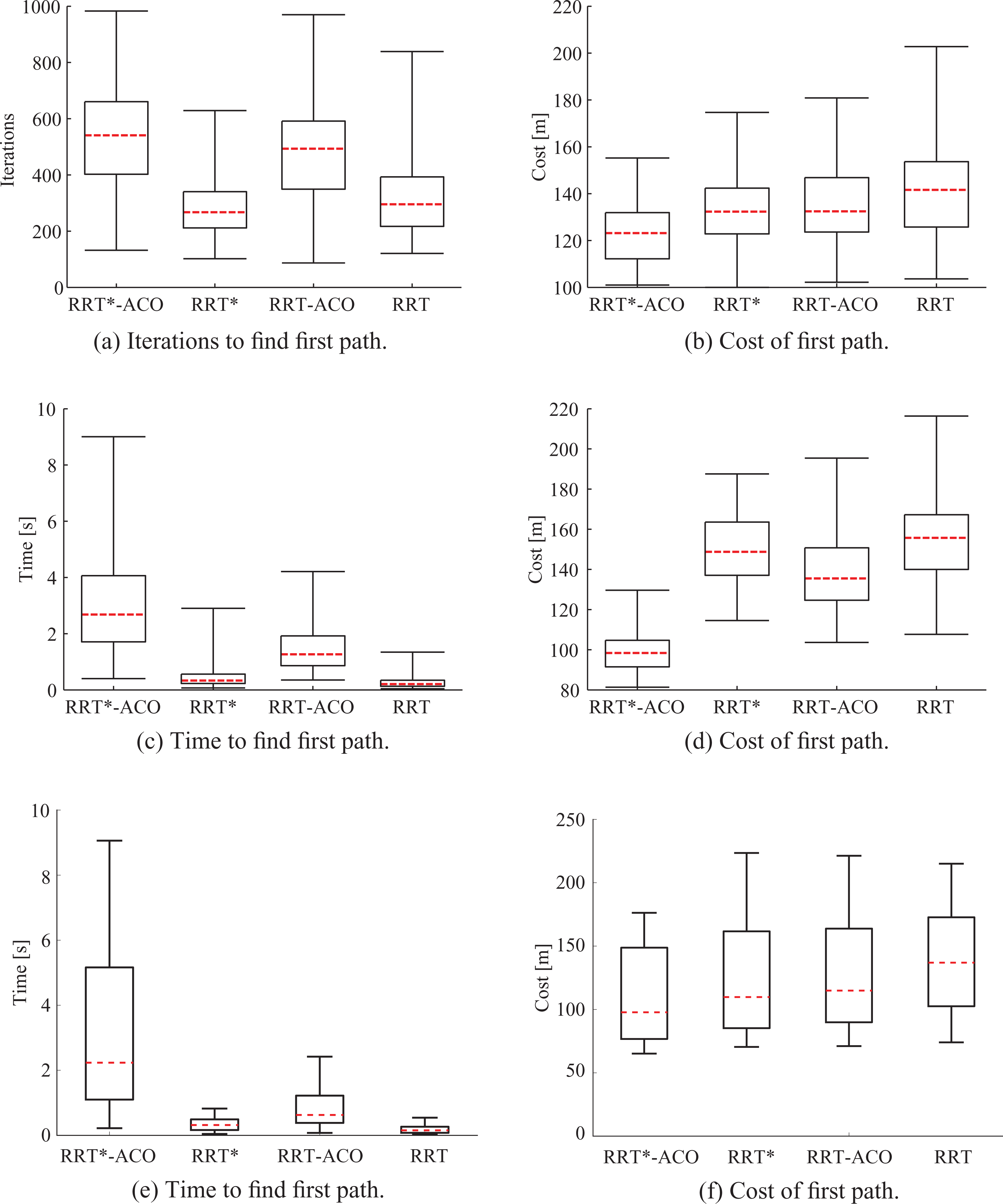
(a, b) Scenario 1. Multiple rectangles. (c, d) Scenario 2. Narrow passage. (e, f) Scenario 3. Maze. Box plot representation of the number of iterations and time to find a first path and its associated cost.

Figure 6 shows a box plot representation of the obtained results, where the dashed red line is the median of the data, the bottom and top of each box represent the 25th and 75th percentiles, and the two strokes encompass the minimum and maximum values. We observe that the ACO-RRT* algorithm finds a better, but slower, solution when compared with the other algorithms. The ACO-RRT* algorithm is slower because the ACO requires some time to place the ants in the best positions to guide the tree’s growth. During the first iterations of the algorithm, the ants are not correctly placed and therefore the planner cannot find a path between the initial and goal position. Conversely, we can conclude that RRT is the fastest algorithm to find a first solution to the path-planning problem, although it has the highest cost. We exploit this capability in our anytime implementation to find rapidly a first solution.

Algorithm performance with time

Once we have found a first path, we aim to improve it to reach the optimal solution. Figure 7 shows the evolution of the best path found over the number of iterations and time. We accompany these figures with a simulation of the algorithm’s complexity for the three scenarios. The results of the proposed ACO-RRT* algorithm are compared with ACO-RRT, RRT* and RRT algorithms.

Figure 7.

(a, b) Scenario 1: multiple rectangles. (c, d) Scenario 2: narrow passage. (e, f) Scenario 3: maze. Evolution of the best path cost over time and iterations after finding a first solution. The right hand side shows an evaluation of the algorithm time complexity. (a) Path cost versus iterations. (b, d, f) Time versus iterations. (c, e) Path cost versus time.

The curves in Figure 7 correspond to the mean value calculated over 100 runs. For each of the curves in Figures 7(a), (c) and (e), we have considered the worst case; that is each of the curves starts when a path was found in all the 100 runs. We observe that the ACO-RRT* algorithm offers a superior performance over time. However, for scenario 3, the performance is similar to the one offered by RRT*. This is because Scenario 3 is more structured and therefore, once the algorithm finds a first solution, it has little room for improvement. These results naturally led us to formulate the anytime ACO-RRT* algorithm. Although the solution offered by the RRT algorithm in the first place is of worse quality, we expect to improve it using ACO-RRT*. We expect this combination to incur an increase in performance over time.

Note that the introduction of the ACO increases the algorithm’s computational complexity. This is mainly because of the time needed to compute the ant’s utility and update the table that contains the ants. However, this additional complexity is beneficial, since the ACO-RRT/RRT* offers a better performance.

Anytime ACO-RRT* performance

Figure 8 shows the performance of the anytime implementation of the algorithm. We would assume that the RRT and anytime curves should start at the same position, since both of them start running the RRT algorithm. However, here we represent the first moment in which we have found a path for all the 100 algorithm runs. They would then start at the same point if the number of runs approaches infinity. This algorithm is the fastest to find a first path (equal to RRT) and has the same evolution of the performance over time (equal to ACO-RRT*).

Figure 8.

Scenario 1: multiple rectangles, anytime ACO-RRT* performance. (a) Box plot representation of the time to find a first path. (b) Evolution of the best path cost over time once we have found a first solution.

Performance with respect to algorithm parameters

For Scenario 1, we evaluated the evolution of the path cost over time with respect to the number of ants, the exploitation–exploration trade-off parameter, and the evaporation rate; while keeping the not-analyzed parameters constant, according to Table 1. We did not simulate the influence of varying q, since this is strongly correlated with k. This allows us to keep q fixed and just modify the number of ants k.

Figure 9 shows the performance with respect to the number of ants. We also performed simulations with a smaller number of ants but the algorithm was not able to converge to any solution in the given planning time. We observe as well that 50 ants corresponds to the best solution. Increasing the number of ants, however, incurs a decrease in performance. The explanation of such behaviour comes from the trade-off that exists between including more ants to better learn the sampling distribution, and the complexity added at the sampling procedure when increasing the number of ants.

Figure 9.

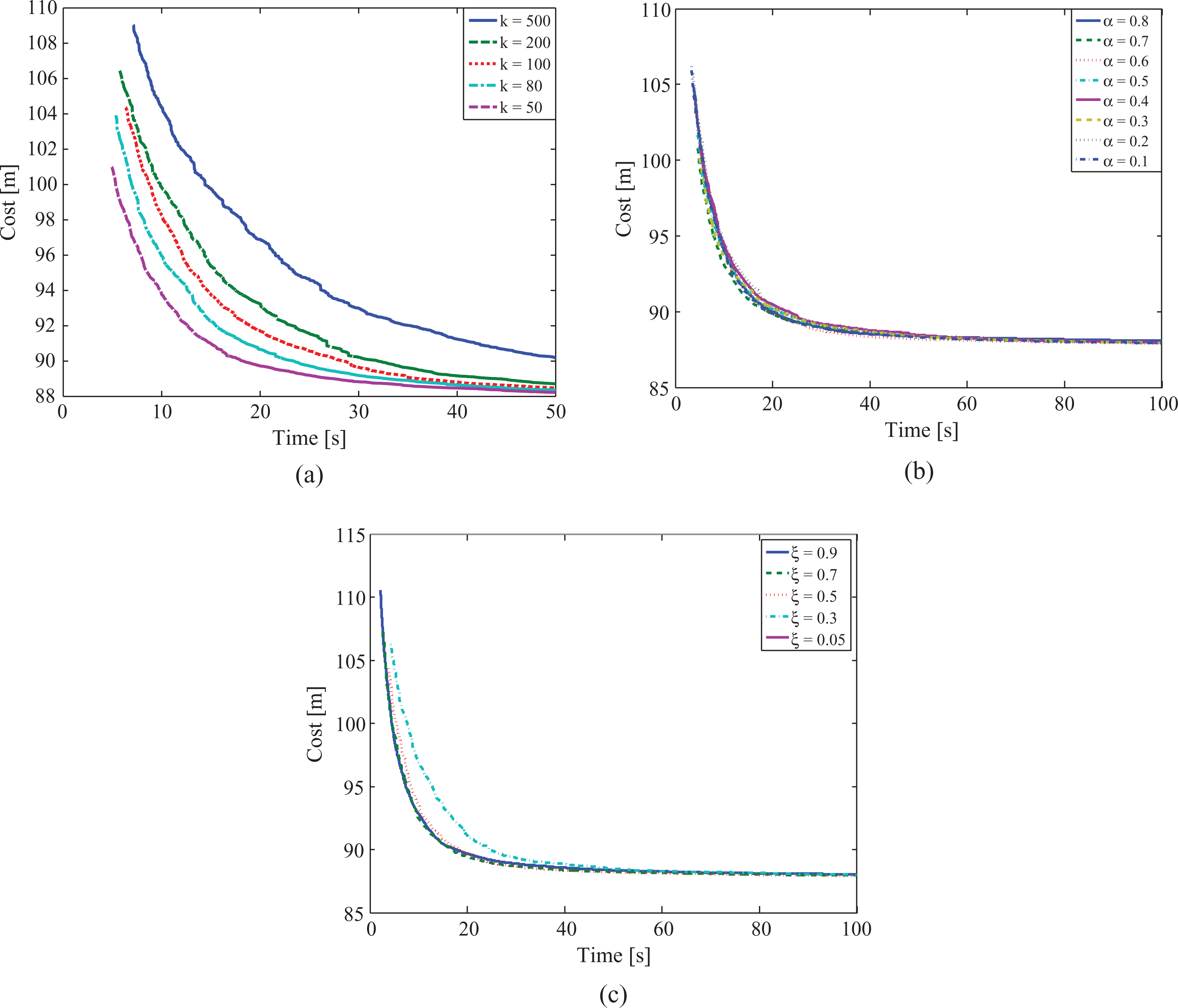
Scenario 1: multiple rectangles; Analysis of the algorithm performance with respect to: (a) number of ants, k; (b) the exploitation–exploration trade-off parameter once we have found a first path, $\stackrel{⌣}{\alpha }$ ; (c) evaporation rate, ξ. Each simulation corresponds to the variation of the specific parameter, while leaving the rest constant according to the values of Table 1.

To analyze the impact of the α factor in the algorithm performance over time, we keep constant $\widehat{\alpha }$ and vary $\stackrel{⌣}{\alpha }$ between 0 and 1 (see Figure 9). As we could expect, for extreme values of $\stackrel{⌣}{\alpha }$ , the algorithm does not find a solution. For the remaining values, the performance varies only slightly.

In Figure 9, we observe as well that the algorithm does not converge only for the extreme values of the convergence rate ξ. As in the previous case, it is important that performance does not drastically change as we vary this parameter.

Examples of paths planned with the ACO-RRT* algorithm

We have analyzed the different parameters that influence the algorithm’s performance. In addition, we include in Figure 10 three snapshots of the paths planned after running our proposed ACO-RRT* algorithm. The figures show the resulting trajectory, the samples that conform the tree, and the ants at the end of the algorithm’s execution. We can observe that most of the ants are placed in the region of the state space that contains the optimal trajectory. This results in the presence of more samples in this region, which is the goal of our algorithm. For Scenario 3, it can be seen that the first path found is already very close to the optimal path.

Figure 10.

Example of one path planned with the ACO-RRT* algorithm for each of the analyzed scenarios: (a) Scenario 1; (b) Scenario 2; (c) Scenario 3. The large pink dot is the starting position. The red square is the goal region. The final path is coloured red. The black dots are the samples generated by the algorithm. The yellow and pink dots represent the ants’ positions at the end of the algorithm’s execution. The ants represented with the pink dots are the ones that were placed on top of an obstacle during the algorithm’s execution.

Conclusions and future work

In this work, we have proposed and analyzed a novel path-planning algorithm (ACO-RRT*) based on rapidly exploring random trees (RRTs). We have modified the RRT algorithm sampling strategy so that the current tree influences the sampling. This is done by defining a novel utility function in combination with the ant colony optimization algorithm. The utility function is defined to trade off between (i) exploiting the current solution and (ii) exploring the states’ space. We have compared the ACO-RRT* algorithm performance with the RRT and RRT* algorithms in three challenging scenarios. The proposed algorithm is able to find a higher quality first path than the other alternatives (improvement factor between a 1.08 and 1.5). In addition, the results suggest that our algorithm approaches the optimal solution 3.6 faster than the RRT* algorithm. However, it takes more time to find the first path. To reduce this time, we extended the algorithm to an anytime version. Here, the algorithm searches a first path as quickly as possible regardless of the path’s cost, and then improves it using the ACO-RRT* algorithm. Simulations results demonstrate that this anytime ACO-RRT* outperforms the state-of-the-art RRT/RRT* algorithms. We also compared the algorithms’ performance, by varying the different parameters that conform the algorithms.

Future steps are to encompass the experimental validation of the algorithm with a robot-in-the-loop. We also aim to learn the optimal algorithm’s parameters. This could be done by reinforcement learning, where the robot could automatically tune these parameters by analyzing the current solutions as it moves. We are working to extend this framework to handle more complex objective functions; for example autonomous exploration and handling model uncertainty. In addition, a future goal is to perform path planning in an environment populated with obstacles and moving agents that can cooperate. In this situation, we believe we could obtain a great improvement by exchanging ants between agents. Here, we have proposed a framework to treat the rapidly exploring random trees algorithm. We believe that incorporating some of the state-of-the-art methods in this framework, by the definition of proper utility functions, will lead to a greatly superior performance.