Sage Journals: Discover world-class research

Abstract

Human hand functions range from precise minute handling to heavy and robust movements. Remarkably, 50% of all hand functions are made possible by the thumb. Therefore, developing an artificial thumb that can mimic the actions of a real thumb precisely is a major achievement. Despite many efforts dedicated to this area of research, control of artificial thumb movements in resemblance to our natural movement still poses as a challenge. Most of the development in this area is based on discontinuous thumb position control, which makes it possible to recreate several of the most important functions of the thumb but does not result in total imitation. This work looks into the classification of electromyogram signals from thumb muscles for the prediction of thumb angle and force during flexion motion. For this purpose, an experimental setup is developed to measure the thumb angle and force throughout the range of flexion and simultaneously gather the electromyogram signals. Further, various features are extracted from these signals for classification and the most suitable feature set is determined and applied to different classifiers. A “piecewise discretization” approach is used for continuous angle prediction. Breaking away from previous research studies, the frequency-domain features performed better than the time-domain features, with the best feature combination turning out to be median frequency–mean frequency–mean power. As for the classifiers, the support vector machine proved to be the most accurate classifier giving about 70% accuracy for both angle and force classification and close to 50% for joint angle–force classification.

Keywords

Electromyogram biosignal processing classification features extraction motion prediction.

Introduction

Among the major factors contributing to the dexterity and versatility of the hand is the uniqueness of the thumb. It is widely claimed by clinicians that more than 50% of all hand functions are made possible by the thumb.¹ It naturally follows that any damage to the hand and more specifically to the thumb will have a negative impact on human functioning. For this reason, many researchers and developers in biomechatronics have invested heavily in producing artificial limbs to be used in cases where there is a complete or partial loss of hand. One of the most successful prosthetic hands created in recent times has been PRODIGITS made by Touch Bionics in Scotland.² This was developed further into the i-Limb Ultra revolution, which is a more advanced prosthetic with features like lighter and more anatomically accurate fingers, powered thumb rotation, added dexterity (up to 24 different grip patterns), and even Bluetooth connectivity.³ Another such advanced prosthetic is the Bebionic3 by RSLSteeper⁴ that has 14 preprogrammed grip combinations for the most common hand movements like typing, precise handling, and so on. It is controlled by the muscle signals generated by the upper arm. However, as is apparent from a survey of the currently available prosthetics, most of the development in this area is based on discontinuous or discrete thumb position (force and angle) control, which makes it possible to recreate many of the most important functions/positions of the thumb but does not result in total imitation. These prosthetics are designed to emulate the movement, design, and performance of a natural hand as closely as possible in order to restore the lost functionality. It is therefore important that an artificial limb be developed that can mimic the actions of a real body part as closely as possible. There have been recent studies in this particular area, such as the one by Park et al.⁵ who suggested the use of biomechanical models to predict the force at the thumb tip based on the surface electromyogram (sEMG) signals. For this, they used the Hill-based muscle model, which uses the processed neural activity, muscle length, and contraction velocity to estimate the force generated by the muscle. This model was applied to five of the nine muscles (the remaining four muscle forces were estimated), and the resultant force at the thumb tip was estimated. Similarly, Ryu et al.⁶ have suggested a way for continuous position control of the wrist joint using a model-free technique. They use a multilayer neural network (NN), which is trained through back propagation to derive a time-continuous relationship between the electromyogram (EMG) signals and the wrist angle, which was then used to control a 1-degree of freedom manipulator. Different studies in recent times, such as the study by Aung and Al-Jumaily,⁷ Khushaba et al.⁸ and Zhang et al.⁹, have used different techniques for EMG classification, all with similar applications in biomechanics. In addition to the aforementioned studies, extensive review papers like those by Tao et al.¹⁰ and Fougner & Stavdahl³¹ have also been written on the subject and gave a very good idea of the general trends in this field.

To further research in the area of continuous thumb position estimation and control, an original experimental setup that measures the characteristic of the thumb motion is proposed. In the experiment, the EMG signal of muscles closely engaged in thumb activity for a certain motion performed under different weight/force categories is recorded and analyzed. The rest of the article is organized as follows: Section “Classification theory” gives a brief background of classification theory and its methods, while section “Experimental setup” explains the experimental setup designed for data collection and the procedure employed for it. Section “Signal processing” describes the EMG signal processing, which includes the process of feature extraction and classification, and section “Results and discussion” presents the results of the processing and its analysis. Finally, section “Conclusion” gives the conclusion and offers some recommendations for future work.

Classification theory

Whenever there are huge amounts of data, they must be intelligently analyzed and the information hidden in them must be sought, if the data is to be used in any meaningful way. This recognition of hidden patterns in huge data sets is known as data mining. Since data in the real world is always adulterated with noise and other irrelevant information, one of the biggest challenges in data mining is the ability to adapt to vastly varying and complex data sets. This permits more intelligent and “human-like” understanding and behavior, making data mining a branch of artificial intelligence with numerous applications in speech and face recognition, character recognition, and so on. In general, data mining combines signal and data acquisition, data preprocessing, feature extraction (data reduction), and “learning.”^11,12

Learning in the context of data mining refers to the ability to comprehend the data in a meaningful way and take decisions based on that. The four main approaches to learning are classification where a set of classified or labeled examples are used to form a scheme to classify unseen examples; association learning where any association within the data is identified regardless of whether there is any class or label attached; clustering that groups data that belong together; and numeric prediction where the learning leads to the prediction of a numeric quantity. In all of the aforementioned techniques, what is learned is called the concept; the outcome of the learning method is the concept description; the individual, independent data that is the input for the learning scheme and an example for the concept is called an instance; and the features or parameters that each value of the instance represents are known as attributes.¹¹

Classification is often referred to as a supervised process as the outcomes or classes of the instances are known and provided to the learning scheme beforehand as opposed to an unsupervised process where the outcomes are not known. Supervised learning being more concept-driven or concept-led is inductive in nature, while unsupervised learning is more data-driven or deductive. Success of the classification process is indicated by how well a learning scheme assigns classes to a set of instances. This is done by first feeding the scheme with a learning data set along with its classes and then testing the scheme on a different data set for which the classes are known but not provided. Many times the classification method is also judged on the basis of how well a concept is learned. In many cases, a particular set of instances may belong to more than one class. Here, the most common approach is to treat them as a series of different classification problems and identify each set of classes individually.¹¹

The classification process for EMG, like for all other applications, begins with feature extraction. This is the process of computing signal attributes and assembling them into a concise vector. It basically does data compression or reduction by removing unwanted or needless information from the raw signal.¹³ Once features have been extracted, the appropriate ones or an appropriate combination of features are selected.¹⁴ This final feature set is a meaningful representation of the EMG data, which is then fed into a classifier. The classification process has multiple stages as shown in Figure 1.

Figure 1.

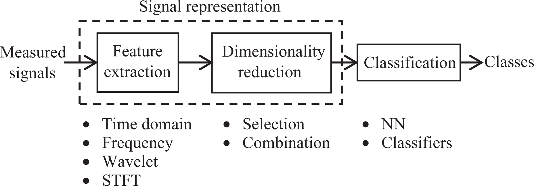
Classification process.

Some of the most commonly used classification techniques are described next.

Neural network

NNs are based on the natural neurotransmission model and are therefore commonly referred to as artificial NNs. One of its most commonly used implementations is the multilayer perceptron that functions on the basis of the back propagation method.¹⁵ It works by having an input layer of nodes that are all connected to all nodes of the following layer. These are in turn connected to the layer following them, and this continues till the last layer which is the output layer. This is depicted in Figure 2(a). The number of layers and nodes varies as per the application and type of data. All connections between the nodes have their own weight, which governs the impact that each input has on the subsequent layer. In this manner, the values are fed forward across the hidden layers to the output layer, which then either directly or through the application of some function give the final output. The weights of the connections are adjusted iteratively based on the accuracy of their outputs. NNs are adept at handling noisy or incomplete data, which makes them suitable for EMG classification. They have been used widely by researchers^16

–19 and three different NN models for EMG classification have been studied.

Figure 2.

Representation for (a) neural networks—top left, (b) SVM—top right, and (c) PART—bottom. SVM: support vector machine; PART: partial decision tree.

Support vector machines

A support vector machine (SVM) works on the idea of finding the maximum-margin hyperplanes that can discriminate between data belonging to different classes. This makes the SVM good at generalizing besides being computationally efficient and robust with large dimension data. The maximum-margin hyperplane is the one that is farthest away from the instance spaces of both classes. This ensures maximum separation between them and results in better classification. The instances that are closest to the maximum-margin hyperplane, that is, are at the edge of their respective class space, uniquely define or “support” it. Hence, the name SVM. This is illustrated in Figure 2(b). SVM also uses a regularization parameter that enables the accommodation of outliers and allows errors on the training set.²⁰ Another crucial advantage is that a linear SVM can make nonlinear decision boundaries using the “kernels.” Kernels map the nonlinear data to a linear space by applying the appropriate functions like radial basis function (RBF), polynomials, or the Pearson VII function-based universal kernel (Puk) as explained by Üstün et al.²¹ One manner of training the SVM is the sequential minimal optimization algorithm that works by breaking down large problems into smaller subproblems. This implementation transforms nominal attributes into binary ones and also normalizes all attributes by default.¹¹

Partial decision tree

A decision tree works using a specific attribute as a basis or root node that then branches out into different values for that attribute. In this way, the data set is split into subsets, one for every value of the attribute. The process is then repeated recursively for each branch, using only those instances that actually reach it. When all instances at a node have the same classification, that part of the tree stops growing. An example of a decision tree to see if the weather is good is shown in Figure 2(c). Decision trees, based on their approach of dividing the data set, are also known as “divide-and-conquer” techniques. There are other techniques that work on the principle of “separate-and-conquer,” that is, a rule is identified that covers many instances in the class (and excludes ones not in the class) and then separates them out. The process then continues with the remaining instances. The “separate” step is more efficient, because here the data set shrinks continually. A partial decision tree (PART) is a combination of both these approaches.¹¹

Experimental setup

As the motion of interest is thumb flexion, it is necessary to have a means of measuring the thumb angle throughout the range of this motion. Therefore, it was decided that two plates—a fixed, flat lower plate aligned to the radial side of the palm (the blade along the index finger) and another movable, flat upper plate aligned with the face of the thumb—that are joined at a hinge, would be used. This design proved to be quite advantageous as it allowed for free, unrestricted thumb motion and easy measurement of the thumb muscles. The motion of the upper plate is caused by the thumb, which means that the angle of the upper plate with respect to the lower plate is almost the exact indicator of the thumb angle caused by flexion. This angle is captured electronically by connecting a potentiometer to the axis of the hinge between the plates. The upper plate is attached to a pulley system that has weights suspended on the other end. The movement of the plate in this case is possible only if the thumb exerted a force to pull the weight and these weights could easily be adjusted to required values (three different weight sets were used for this study). The desired results for this experiment are the precise measurement of thumb position and EMG signals for each weight/force category during a flexion motion. To this end, the following guidelines and method were employed to conduct the experiment. The entire arrangement is illustrated in Figure 3.

Figure 3.

Experimental apparatus for data collection.

Angle measurement

Measurement of the angle was done in an effective manner using a rotary potentiometer. As the potentiometer is attached to the rotating axis of the hinge between the upper and lower thumb plates, its axis of rotation coincided with the joint between the thumb and palm. This is the joint around which thumb flexion takes place. Therefore, the rotation of the potentiometer provided an accurate measure of the thumb angle. The potentiometer had a range of 2 MΩ and is supplied with 0–5 Voltage DC (VDC) for power. The varying output of the potentiometer is sent to a 741 operational amplifier-based isolation amplifier or buffer with a −5 to 5 VDC power supply.

Force measurement

There were two different techniques available for measuring the force varying through the thumb motion. The first one, which was considered originally, was to get the actual force exerted by the thumb tip as it went through the flexion. This was made possible by embedding a force sensor in a specially designed groove in the upper plate (the small, black, circular device in the upper plate—as shown in Figure 3). The force sensor was placed such that the thumb tip would press down on the sensor in order to flex and press the upper plate downward. A cursory look at the force readings showed highly erratic and inconsistent behavior that would not be helpful in further processing or classification. The other technique, which was the one adopted, was to use different weight sets attached to the upper plate as a force/weight class by themselves. This meant that each weight set would be considered a different class. The experiment was carried out with six different weights, ranging from 100 g to 600 g. However, for the purpose of classification, two adjacent weights (100–200 g, 300–400 g, and 500–600 g) were taken as a single class, resulting in a final three classes.

EMG measurements

The EMG signals were acquired through the g.USBAmp, which is a biosignal acquisition and amplification device from gtec, Austria. For EMG acquisition, the sampling rate is set to 1200 Hz, and a high-pass filter with a cut-off at 2 Hz was used to remove the white noise, while a 50 Hz notch filter was used to remove power line disturbances.

Subject preparation and electrode placement

For EMG recording, the body of the subject is connected to the common ground to reduce noise and disturbances. The reference electrode for the gtec amplifier was placed on the wrist of the subject, while the ground electrode was placed on the elbow bone. The electrodes for the muscles were placed on the first dorsal interosseous located on the backside of the palm near the thumb joint, the flexor pollicis brevis located in the thenar eminence (the slight bulge in the palm at the base of the thumb), and the extensor pollicis brevis located in the forearm behind the thumb (as shown in Figure 4). Subjects were instructed to start the motion by moving the thumb from the vertical to the horizontal position in a slow, steady, and constant speed. Subjects were asked to hold their thumb at the maximum horizontal position for about 3 s before moving it back up to the original vertical position. This completed one trial of the motion, after which the subjects moved the thumb to a position of rest. A total of five male subjects were used in this study, all of whom were right handed. A minimum of five trials were done for each subject with a gap of about 5 s after each trial.

Figure 4.

Electrode placement.

Signal processing

Segmentation

Segmentation is to divide the continuous thumb movement into smaller sections or segments. For this particular case, the thumb flexion movement was divided into three segments. Here, the entire movement was divided into segments based on fixed intervals of the thumb angle. As a result, the entire flexion movement, ranging from 90° (where the thumb is perpendicular to the ground) to 0°, was divided into three intervals—the first and last segments covering 22.5° each and the middle segment covering 45° (this was done as the movement in the middle tends to be faster than at the extremes). Next, corresponding segments in each trial for a particular angle interval were concatenated together to form a data set or population/class (inclusive of all trials) for that specific angle interval. The same was done for all intervals and weight categories, resulting in a total of nine classes—three angle classes for each of the three force/weight categories. Each class of data was further divided into subsegments of hundred samples each. Each of these subsegments is treated as a separate section for time-domain (TD) feature extraction. For the calculation of frequency-domain (FD) features, however, subsegments of 512 samples with a 50% overlap were used. This is because the FD transform is dependent on Fast Fourier Transform (FFT), which requires the subsegment length to be a power of 2. A typical representation of thumb angle segmentation and the EMG signals for one segment is shown in Figure 5.

Figure 5.

Angle segmentation and corresponding EMG signals for segment 1, trial 1. EMG: electromyogram.

In an effort to further improve results, an alternative approach to segmentation was also tried, the details of which have previously been presented in the study by Siddiqi et al.²² The basic difference was that instead of having two smaller segments of 22.5° and a large mid-segment that covers 45° of motion, the entire motion was divided into three equal segments covering 30° each. The effect of this segmentation is presented and discussed in the Results section here as well, in order to compare the performance of the two segmentation approaches and highlight the difference between them.

Feature extraction

Feature extraction is the transformation of raw signals into a set of parameters that represent the signal. This transformation causes dimensionality reduction.²³ TD features are computed based on signals’ amplitude and do not require any complex calculation, whereas FD features are based on the frequency spectrum and are computed based on the Fourier transform. To have a discriminant representation of the EMG data, linear prediction (LP) along with other commonly employed time and FD features are applied to the data. These features have been discussed earlier in various works like those of Refs. ^23

–28. The commonly used TD features are LP coefficients (AR coefficients) and its error variance, Willison amplitude (WAMP), mean absolute value (MAV), simple square integral (SSI), modified MAV1, modified MAV2, slope sign changes, variance of the signal, waveform length (WL), standard deviation, difference absolute standard deviation value, zero crossing, skewness, and root mean square. The most common FD features include mean frequency (MNF), peak frequency, median frequency (MDF), mean power (MNP), and power spectrum ratio. The definitions and mathematical derivations for these commonly used features are given in the Appendix.

Selection of an effective subset of features is the most important factor in achieving high accuracy in results. For this purpose, the performance of each feature was first evaluated individually and the best-performing feature was used as a base to build the final feature set. A cursory examination of the accuracies achieved by different features revealed that the FD features fared better than the TD features, especially in force classification. This is possibly due to the short time window of the signal. Hence, the final feature set was built on only the FD features and their combinations. The features that form the base of the feature set include MNF, MDF, and MNP. A sample of the results that led to this conclusion is shown in the following section.

Classification

Classification, the last step in processing, is the process of identifying the class or category to which an observation belongs. This process of identification is carried out by training the classifier model using a set of data where the classes or categories are known. In this study, three different classification methods are applied to the extracted features. Each of the classifiers has a different approach or algorithm to assign a particular class to a new observation. The performances of these classifiers are compared based on the average accuracy achieved after a 10-fold cross-validation, that is, where the data is divided into 10 folds of equal size and at each iteration, 9 folds are used for training the classifier, while the tenth is used for testing. The test results of all iterations are averaged over all folds to obtain the cross-validation accuracy. The different classifiers employed were implemented using WEKA.¹¹ The selected classifiers are NNs, SVM (with Puk), and PART. Furthermore, there are two different approaches to use these classifiers—the first is the joint angle–force approach where both are estimated simultaneously and the other is where angle and force classification is done separately. Results for both are given in section “Results and discussion.”

Overall scheme

The general scheme followed for data processing starts with the segmentation of the thumb motion to match different force and angle classes. This means that the entire thumb motion is divided in a manner that each segment corresponds to a specific weight and force category or class. The angle category or class is determined by the angle intervals derived from the segmentation process, while the force/weight class is taken from different weight sets used. Different features were then extracted from sample windows (100 samples for TD and 512 for FD) of these segments and used as inputs for the classification of the different angle and force/weight classes. The results of the classification form the basis for establishing the most appropriate features, classifier, and overall strategy (joint or individual classification). The overall scheme for a single weight class is illustrated in Table 1.

Table 1.

Illustration of overall processing scheme.

	Number of samples in angle segment
Trial number for wt. class A (100–200 g)	1 (0–22.5°)	2 (22.5–67.5°)	3 (67.5–90°)
1	400	400	800
2	400	400	500
3	400	400	400
4	500	400	800
5	500	1200	2000
Data set size	2200	2800	4500
Number of TD windows (100 samples—disjoint)	22	28	45
Number of FD windows (FD-512 samples—overlapped)	7	10	16

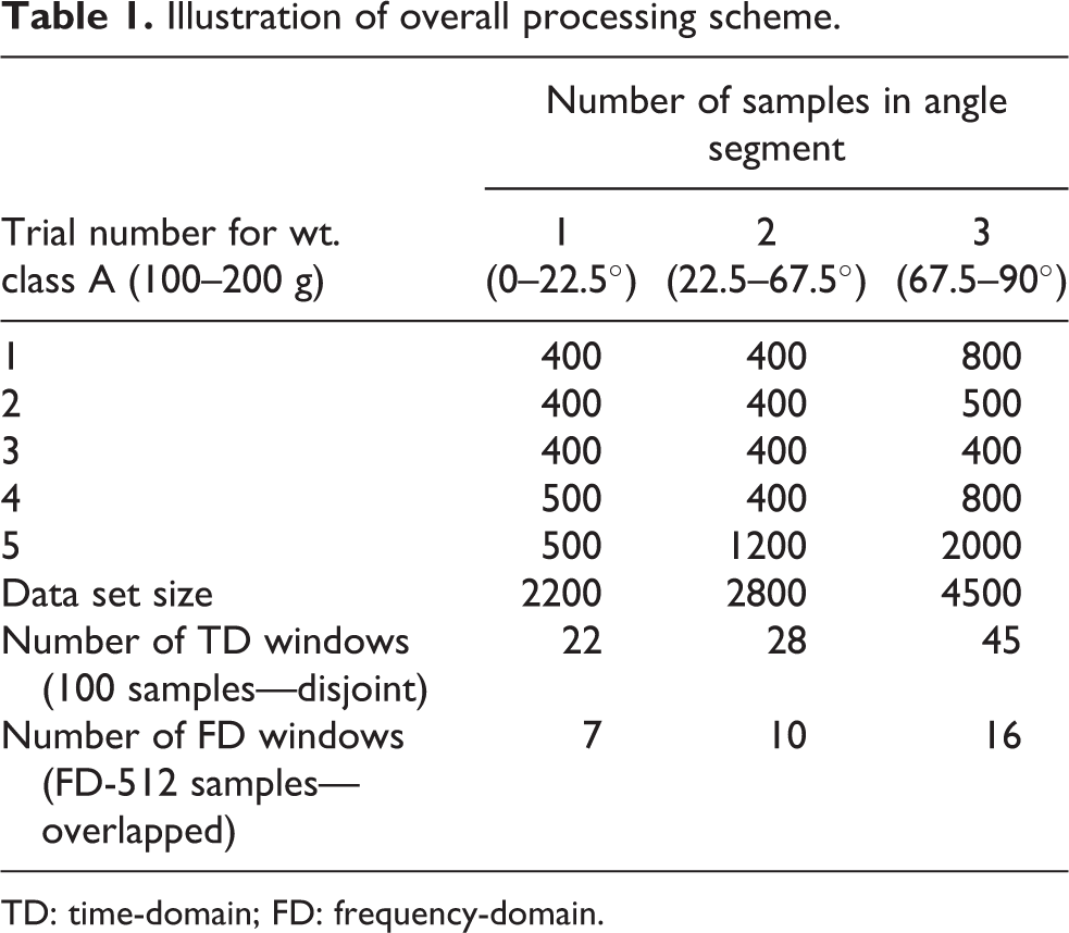
TD: time-domain; FD: frequency-domain.

In the aforementioned illustration, 22 instances of different TD features and 7 instances of different FD features are extracted from the windows (or subsegments) of the first angle segment for this particular weight class. So, the result is 22 values of each TD feature, like MAV, WAMP, and so on, and 7 values of each FD feature, like MNF, MDF, and so on, that form the input to the classifier, while angle class 1 (0–22.5°) and weight class A (100–200 g) form the outputs.

Results and discussion

Feature set finalization

To reach a decision on the final feature set, different TD and FD features were applied, individually and in combination, to a standard classifier and their accuracies were compared. The classifier used here was the NN model. An indicative sample of the results is shown in Table 2. As the base for the TD feature set was the AR coefficients, they were included in all combinations.

Table 2.

Results for time-domain and frequency-domain features.

Time domain features			Frequency domain features
Feature	Fr/Wt	Angle	Feature	Fr/Wt	Angle
AR–1*	35.13	56.16	MDF–MNF	34.15	51.93
AR–2	35.76	57.14	MNF–MNP	36.18	55.63
AR–3	35.95	55.88	MNF–MNP	37.02	59.10
AR–4	35.58	56.86	MDF–MNF–MNP	38.06	61.06
AR–1–2	35.25	57.10
AR–1–3	35.22	56.28
AR–1–4	36.20	57.56
AR–2–3	36.50	57.02
AR–2–4	36.80	57.51
AR–3–4	36.94	57.89
Average	35.93	56.94	Average	36.35	56.93
Maximum	36.94	57.89	Maximum	38.06	61.06

*Note: 1: MAV; 2: WL; 3: DASDV; 4: WAMP.

Considering the fact that the highest accuracy in both angle and force classification was achieved by a FD combination and also seeing that the average accuracy is either the same or greater for FD features, they were deemed to be the most appropriate to be included in the final feature set.

Final results

The average accuracy achieved across subjects for joint angle and force classification using the different classifiers is given in Table 3, while the average accuracies achieved for individual angle and force/weight classification are given in Table 4.

Table 3.

Summary of joint classification results.

Feature	NN	PART	SVM	Average	Maximum
MDF–MNF	40.54	33.16	42.99	38.89	42.99
MNF–MNP	48.24	50.29	53.35	50.62	53.35
MNF–MNP	52.08	52.09	57.76	53.98	57.76
MDF–MNF–MNP	52.93	53.35	57.11	54.46	57.11
Average	48.45	47.22	52.80	49.49	52.80
Maximum	52.93	53.35	57.76	54.46	57.76

NN: neural network; PART: partial decision tree; SVM: support vector machine; MDF: median frequency; MNF: mean frequency; MNP: mean power.

Table 4.

Summary of individual angle and force classification results.

	Angle classification
Feature	NN	PART	SVM	Average	Maximum
MDF–MNF	59.90	56.32	65.11	60.44	65.11
MNF–MNP	71.20	72.99	74.38	72.86	74.38
MNF–MNP	76.55	75.03	78.43	76.67	78.43
MDF–MNF– MNP	75.39	75.27	76.57	75.74	76.57
Average	70.76	69.90	73.62	71.43	73.62
Maximum	76.55	75.27	78.43	76.67	78.43
	Force classification
Feature	NN	PART	SVM	Average	Maximum
MDF–MNF	58.13	53.40	63.16	58.23	63.16
MNF–MNP	59.82	63.29	65.94	63.02	65.94
MNF–MNP	61.97	63.60	67.95	64.51	67.95
MDF–MNF– MNP	64.15	63.47	69.31	65.64	69.31
Average	61.02	60.94	66.59	62.85	66.59
Maximum	64.15	63.60	69.31	65.64	69.31

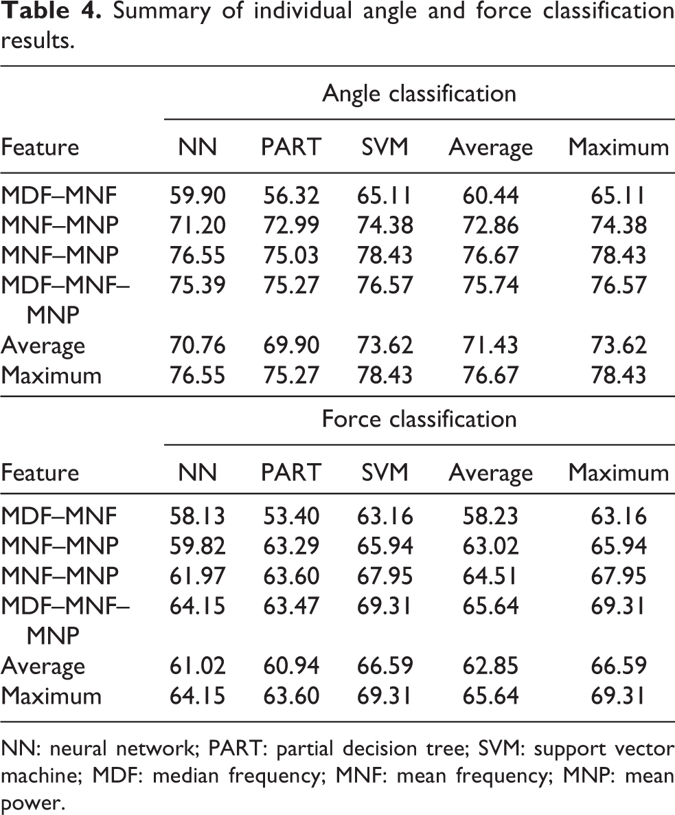
NN: neural network; PART: partial decision tree; SVM: support vector machine; MDF: median frequency; MNF: mean frequency; MNP: mean power.

The results from individual classification yield much better results than joint classification. The angle classification accuracy, when done individually, is around 70% for all classifiers with the average being 71.43%. The best performing classifier is SVM and the best feature combination here is MNF–MNP that gives the highest accuracy of 78.43%. For force classification, the average accuracy is 62.85% across different classifiers with the highest average accuracy shown by SVM (66.59%). The best performing feature here is MDF–MNF–MNP giving 69.31%. For joint classification, MNF–MNP gives the best accuracy (57.76%), with the MDF–MNF–MNP combination giving a strikingly close result. Even for joint classification, the best performing classifier turns out to be SVM and the best performing feature combination is MNF–MNP. However, based on average accuracy, the MNF–MDF–MNP combination is better for joint classification.

The markedly better performance of individual force/angle classification as compared to joint classification was expected as the classifier deals with only three classes at a time in the first case and with nine classes in the latter. Obviously, the chances for misclassification are significantly greater in joint classification. Another interesting, but not expected, attribute of the results was the FD features performing better than the TD ones. There could be different explanations for this, the first being that the motion being studied is continuous as opposed to a stationary posture. This might cause more variation and consequently more unpredictability in the temporal EMG signal, making the frequency spectrum more useful. It is also possible that the FD provides more determinant features since the motion, especially in the case of varying force/weights, is closely associated with the firing rate of the EMG signal. It is even possible, although not very likely, that the difference in the segment size for different feature sets has an effect on the performance. These reasons need to be explored further and warrant a separate study of their own.

The SVM classifier seems to be well suited to this application, first because of its relatively better performance and also for its ability to sharply demarcate adjacent classes. In this particular case, even a misclassification between instances that are close by in adjacent classes might not affect the overall performance of the final system. This is because the motion being predicted is continuous and so follows a path that goes through all the classes (angle intervals) sequentially. So, a mistake in identifying the adjacent classes (angle intervals) will not have a major impact on the motion path. So, it is safe to assume that the SVM will produce even better results in actual application. The use of a supervisory controller or classifier that takes into account the previous instances will also greatly improve the accuracy.

Alternative segmentation

The alternative segmentation strategy was applied to angle classification as that is where its effect would be most prominent. The approach followed to build a feature set here was roughly the same. First, a base for the feature was selected, and then based on the effect of different features on the overall classification accuracy, the most contributing features were made part of the final set. Thereafter, different combinations of these features were used for the classification process. It is noteworthy that the best performing features here were the TD features.

Although, the fourth-order Auto Regressive (coefficients) (AR) has been suggested in earlier research,²⁹ an investigation is done on the AR model order that best fits this specific recorded data and results in higher classification accuracy. To provide a uniform standard for assessing the accuracies, a simple logistic classifier with 10-fold cross validation is used to build the feature set. Different orders of AR coefficients (along with the respective error variance) are tested and comparing the results leads to the selection of the second-order AR coefficients as the base feature. The features that affect the accuracy positively are subsequently included in the feature set, and these include modified Willison amplitude (MWAMP), SSI, and WL. A summary of the results achieved through this approach (with different classifiers) is presented in Table 5.

Table 5.

Summary of classification results—alternative segmentation.

Feature	Simple logistic	SVM	NN	Naïve Bayes	Average
AR	85.72	84.68	82.21	83.95	84.14
AR–MWAMP	86.22	86.42	83.87	84.43	85.23
AR–SSI	85.82	86.46	84.04	85.32	85.41
AR–MWAMP–SSI	85.01	87.55	85.02	83.88	85.37
AR–MWAMP–SSI–WL	84.14	87.55	84.97	84.04	85.18
Average	85.38	86.53	84.02	84.32

SVM: support vector machine; NN: neural network; MWAMP: modified Willison amplitude; SSI: simple square integral; WL: waveform length.

It becomes evident from the results that equal segmentation results in a much better accuracy of classification. Also notable is the fact that TD features perform better than the FD features here. Overall, the maximum average accuracy, 87.55%, is achieved by SVM using the AR–MWAMP–SSI and AR–MWAMP–SSI–WL combinations. The least accurate results were given by the RBF–NN using just Auto Regressive (2nd Order) with (error) Variance (AR(2)-Vr), managing an average accuracy of 82.21%. Different classifiers performed best with different features; however, the SVM classifier performed better than the others consistently as was the case earlier.

Conclusion

From this study, it can be concluded that the piecewise discretization approach to classification of continuous data is promising and shows good results. The most appropriate feature set determined in this study, based on results from different classifiers, is MNF–MNP for angle classification and MNF–MDF–MNP for force and joint classification. In the equal segmentation approach, the best feature set for angle classification was determined to be AR–MWAMP–SSI–WL. The best performing classifier in all situations is found to be SVM with Puk. A likely course of action for future work in this area would be to expand this study further using a larger number of subjects. Moreover, the types of motion studied should also be increased to include different positions and postures. In processing, various combinations of features should be evaluated based on their performance in a number of different classifiers. A possible approach to the study of joint force/angle estimation could be to utilize two parallel schemes simultaneously, one for force classification and the other for angle. As is abundantly clear, different methods for segmentation, feature extraction, and classification yield vastly different results for different objectives. Therefore, it would be prudent to not adopt a uniform approach for all cases. Another important research topic to pursue in classification would be to study the effect of EMG segment size on the accuracy of TD and FD features.

Footnotes

Acknowledgments

The work presented was carried out in the Biomechatronics Research Laboratory of International Islamic University Malaysia. The authors wish to gratefully acknowledge the grant funding from the Ministry of Higher Education Malaysia (SF15-015-0065).

Declaration of conflicting interests

The author(s) declared no potential conflicts of interest with respect to the research, authorship, and/or publication of this article.

Funding

The author(s) received no financial support for the research, authorship, and/or publication of this article.

Appendix—Features derivation

Linear prediction (LP): LP is one of the basic techniques for removing signal redundancy. It approximates the value of the current sample y(n) as a linear combination of past samples. The mathematical expression for this parameter is given by

where a_i are the LP coefficients (LPCs), $\hat{y} (n)$ is the predicted signal, y(n − i) is the ith previous sample of the EMG signal, and P is the prediction order. The error between the actual sample and the predicted sample is

According to LP analysis, the EMG is described in terms of the all-poles filter coefficients and the prediction error. Prediction error is characterized by its variance defined by

where $\bar{e}$ is the arithmetic mean of the prediction error vector e.

Modified Willison amplitude (MWAMP): WAMP counts the number of times that the absolute value of difference between EMG signal amplitude of two consecutive samples exceeds a predetermined threshold value. The threshold value is defined by the method proposed in the study by Khorshidtalab et al.³⁰

Mean absolute value (MAV): This parameter estimates the MAV of each segment by adding the absolute value of all the values x_i –ith point, the current point, of signal x- and dividing it by the length of the segment

Log detector (log): This feature estimates the muscle contraction force that is defined as

Simple square integral (SSI): SSI calculates the energy of EMG signal according to

Modified mean absolute value1 (MMAV1): MMAV1 is an extension of MAV method using the defined weighting function w(i)

Modified mean absolute value2 (MMAV2): It has a continuous weighting function of w(i). This function is known as an improvement to the modified version of MAV

Modified slope sign changes (MSSC): Slope sign changes represent the number of times that the slope of waveform changes its sign. This parameter is a measure of frequency information in TD. The required threshold meant to reduce the noise is defined through the method described in the study by Khorshidtalab et al.³⁰ Given three consecutive samples, x_i − 1, x_i , and x_i + 1, the slope sign change is incremented if

and

Variance (VAR): VAR is a measure of the variation of data points with respect to the mean. It depicts the extent to which the data are spread around its mean

Waveform length (WL): WL is the cumulative length of the waveform over the segment. It indicates a measure of waveform amplitude, frequency, and duration all within a single parameter

Standard deviation (STD): This feature represents the deviation of the mean for each segment

Difference absolute standard deviation value (DASDV): This parameter is the standard deviation value of the wavelength, and it is defined as

Zero crossing (ZC): ZC is the rate of sign changes along a signal. This parameter is a measure of frequency information of the EMG signal that is defined in TD. It is a number of times that amplitude values of the signal cross the zero amplitude level.

Skewness: This parameter measures the degree of deviation from the symmetry of a normal distribution. This measure has the value of zero when the distribution is completely symmetrical or some nonzero values when the EMG distribution is asymmetrical with respect to the baseline

Root mean square (RMS): RMS is an effective, widely used feature for a variety of biosignals including EMG. RMS is a particular case of v-order. V-Order (V) is a nonlinear detector that implicitly estimates muscle contraction force. An optimal value for v has been reported to be 2, which leads to the definition of RMS feature

Note: In all equations, N is the length of the segment, k is the current segment, x_i is the current point of signal, and i is the index of the current point.

Mean frequency (MNF): MNF is the average frequency of the signal. It is calculated as the sum of the product of the power spectrum and frequency divided by the total sum of the spectrum intensity. It is also known as the central frequency (fc). It is expressed as

where f_i is the frequency of the spectrum at frequency i, P_i is the power spectrum at frequency i, and M is the length of the frequency bin.

Median frequency (MDF): MDF is the frequency at which the power spectrum density is split into two equal halves; in other words, MDF is half of the total power. It can be expressed as

Peak frequency (PKF): PKF is the frequency that holds the maximum power (Biopac Systems, Goleta, CA, USA). It is given by

Mean power (MNP): MNP is the average power of the power spectrum (Biopac Systems). It is calculated as

Total power (TTP): TTP, also known as energy, is the aggregate of the full power spectrum (Biopac Systems). The definition is given by

Frequency ratio (FR): FR was proposed to distinguish between contraction and relaxation of muscles in the frequency domain. It is the ratio between the low-frequency and the high-frequency components of the signal. The equation is defined as

where LFB and HFP are the low-frequency band and high-frequency band, respectively. The threshold for dividing the high and low frequencies is decided either experimentally or using the MNF.

Power spectrum ratio (PSR): PSR is a combination of PKF and FR. It is defined as the ratio of the energy P₀, which is near the maximum power spectrum value, to the total energy of the power spectrum. It is calculated by

where n is an integral limit for PKF.

References

MDGuidelines. Burn of wrist and hand, http://www.mdguidelines.com/burn-of-wrist-and-hand (accessed 4 February 2015).

Eisenberg

. Grabbing gracefully, with replacement fingers, http://www.nytimes.com/2010/04/11/business/11novel.html?_r=4& (2010, accessed 4 February 2015).

Melanson

. Touch Bionics’ latest ‘i-limb’ offers a powered rotating thumb, smartphone controls, http://www.engadget.com/2013/04/11/touch-bionics-ilimbultra-revolution-hand/ (2013, accessed 4 February 2015).

RSLSteeper. Bebionic3, http://bebionic.com/the_hand/features (accessed 4 February 2015).

Park

Kwon

Lee

. Real-time thumb tip force predictions from noninvasive biosignals and biomechanical models. Int J Precis Eng Manuf 2012; 13(9): 1679–1688.

Ryu

Han

Kim

. Continuous position control of 1 DOF manipulator using EMG signals. In: 3rd international conference on convergence and hybrid information technology,ICCIT’08, November 2008, Vol. 1, pp. 870–874. Busan, South Korea: IEEE, 2008.

Aung

Al-Jumaily

. sEMG based ANN for shoulder angle prediction. Procedia Eng 2012; 41: 1009–1015.

Khushaba

Kodagoda

Takruri

. Toward improved control of prosthetic fingers using surface electromyogram (EMG) signals. Expert Syst Appl 2012; 39(12): 10731–10738.

Zhang

Hou

Z-GZ

. sEMG-based continuous estimation of joint angles of human legs by using BP neural network. Neurocomputing 2012; 78(1): 139–148.

10.

Tao

Xie

Zhang

. Review of EMG-based neuromuscular interfaces for rehabilitation: elbow joint as an example. Int J Biomechatron Biomed Robot 2013; 2(2/3/4): 184.

11.

Mark

Eibe

Geoffrey

. The WEKA data mining software: an update. ACM SIGKDD Explor Newslett 2009; 11(1): 10–18. WEKA 3, developed by Machine Learning Group, University of Waikato, New Zealand.

12.

Marques De Sa

JP.

Pattern recognition: concepts, methods, and applications. Springer Science & Business Media, Springer-Verlag Berlin Heidelberg New York, 2001.

13.

Kil

Shin

. Pattern recognition and prediction with applications to signal characterization. Washington: American Institute of Physics, 1996.

14.

Englehart

Hudgins

Parker

. Classification of the myoelectric signal using time-frequency based representations. Med Eng Phys 1999; 21(6): 431–438.

15.

Zecca

Micera

Carrozza

. Control of multifunctional prosthetic hands by processing the electromyographic signal. Crit Rev Biomed Eng 2002; 30(4–6): 459–485.

16.

Farry

Walker

ID,

Baraniuk

. Myoelectric teleoperation of a complex robotic hand. IEEE Trans Robot Automat 1996; 12(5): 775–788.

17.

Khushaba

Al-Jumaily

. Fuzzy wavelet packet based feature extraction method for multifunction myoelectric control. Int J Biol Med Sci 2007; 2(3): 186–194.

18.

Al-Assaf

Al-Nashash

. Surface myoelectric signal classification for prostheses control. J Med Eng Technol 2005; 29(5): 203–207.

19.

Abou-Chadi

Nashar

Saad

. Automatic analysis and classification of surface electromyography. Front Med Biol Eng 2001; 11(1): 13–29.

20.

Burges

. A tutorial on support vector machines for pattern recognition. Data Min Knowl Disc 1998; 2(2): 121–167.

21.

Üstün

Melssen

WJ,

Buydens

. Facilitating the application of support vector regression by using a universal Pearson VII function based kernel. Chemometr Intell Lab Syst 2006; 81(1): 29–40.

22.

Siddiqi

Sidek

SN,

Khorshidtalab

. Signal processing of EMG signal for continuous thumb-angle estimation. In: 41st annual conference of the IEEE industrial electronics society (IECON 2015), Yokohama, Japan, 9–12 November 2015.

23.

Rechy-Ramirez

. Stages for developing control systems using EMG and EEG signals: a survey. Technical Report, CES-513 in School of Computer Science and Electronic Engineering, University of Essex, United Kingdom, 2011.

24.

Englehart

Hudgins

. A robust, real-time control scheme for multifunction myoelectric control. Biomed Eng IEEE Trans 2003; 50(7): 848–854.

25.

Bronzino

. The biomedical engineering handbook, Vol. 1. Boca Raton: CRC Press, 1995.

26.

Phinyomark

Limsakul

Phukpattaranont

. A novel feature extraction for robust EMG pattern recognition. Journal of Computing, arXiv preprint arXiv:0912.3973, 12 2009, 1(1), pp 71–80.

27.

Huang

Chen

. Development of a myoelectric discrimination system for a multi-degree prosthetic hand. In: Proceedings of 1999 IEEE international conference on robotics and automation, 1999, Vol. 3, pp. 2392–2397. Detroit, MI, USA: IEEE.

28.

Chu

Moon

Mun

. A real-time EMG pattern recognition system based on linear-nonlinear feature projection for a multifunction myoelectric hand. Biomed Eng IEEE Trans 2006; 53(11): 2232–2239.

29.

Paiss

Inbar

. Autoregressive modeling of surface EMG and its spectrum with application to fatigue. Biomed Eng IEEE Trans 1987; BME-34(10): 761–770.

30.