Sage Journals: Discover world-class research

Abstract

In micro-line segments machining, transition curves with high harmonic components are more prone to causing vibration issues in the feed drive system, which affects machining efficiency and quality severely. To construct low harmonic trajectories, this paper proposes a corner smoothing algorithm that uses the Trajectory Pattern Method (TPM). The transition curve construction and axial motion scheduling are performed with a specified fundamental frequency in one step, which reduces the smoothing process time and avoids excitation of natural modes of vibration of the system. The synthesized trajectories and axial kinematic profiles are all smooth and only contain the selected fundamental frequency and its first two odd harmonics, which minimizes the number of high harmonic components in the required actuation forces/torques and avoids excitation of the system modes of vibration. Linear programming is used to synthesize the trajectories. The proposed algorithm is shown to achieve near time-optimal trajectories. The provided experimental analysis and comparisons demonstrate that the proposed algorithm achieves smooth axial kinematic profiles with low harmonic contents, which would improve machining efficiency and quality.

Keywords

Trajectory pattern method low harmonic vibration corner smoothing axial motion planning

Introduction

The most common practice in CNC machining is to express tool paths by small line-segments. Research work into high-speed and high-quality machining has concentrated on methods to improve smoothness of trajectories. To this end, several researchers have investigated methods for smooth tool path generation.^1,2 Some researchers have focused on the Local Smooth Method (LSM), in which transition curves are constructed at the junction of small line-segments to improve corner smoothness and velocity since it is simple to implement and is easily controlled. For example, Lv et al.³ used arcs to blend small line-segments. Zhang et al.⁴ constructed transition curves with quintic polynomials and Ernesto and Farouki⁵ used rational quadratic Bézier curves. These three algorithms, however, only provide G1 continuity, that is, continuous velocity, at the corner, which would lead to vibration caused due to the present normal acceleration. To obtain G2 continuity, that is, continuous curvature, Du et al.⁶ smoothed small line-segments with cubic Bézier curves. The calculation of a proper transition length, however, requires a significant amount of time. To reduce vibration during the machining process, Pythagorean-Hodograph (PH) spline has drawn a lot of attention for corner smoothing studies because it provides analytical solution of arc-length related to spline parameters. Shi et al.^7,8 developed corner smoothing algorithms for multi-axis tool paths based on quintic PH splines, which avoided the approximation errors of arc-length calculation. In order to simultaneously achieve real-time interpolation and higher order continuous motion, Hu et al.⁹ proposed a C3 continuous analytical corner smoothing algorithm by inserting the specially designed micro PH splines among linear tool path segments. Then, Hu et al.¹⁰ extended the algorithm to construct C3 continuous trajectories for five-axis machine tools. Fan et al.¹¹ enhanced the continuity further by utilizing two quartic Bézier curves to achieve G3 continuity, that is, smooth curvature. Smooth transition curves and tangential motion profiles can be achieved by above algorithms. However, the methods require two computational steps. In the first step, parametric curves are used at the corners to construct the transition schemes. In the second step, tangent motion profiles are scheduled based on the synthesized trajectories. These algorithms are therefore inefficient. In addition, sudden changes in the axis velocity, acceleration, and/or jerk profiles are encountered since only tangential kinematic limits are considered.

In recent years, one LSM has drawn researchers’ attention, in which in one step, the transition schema construction and motion scheduling are performed. Biagiotti and Melchiorri¹² smoothed tool paths using finite impulse filters. The method, however, leads to large contour errors and unavoidable time delay. Tajima and Sencer¹³ developed a direct axis motion profile blending approach to obtain transition curves. Sudden changes in axis jerk may, however, occur at corners due to the use of a method based on jerk-limited acceleration and deceleration process. Zhang and Du¹⁴ used a jounce-limited velocity planning method to achieve transition curves and smooth axis acceleration profiles, but axis jerk profiles are still not smooth.

It is important to note that when expressed in Fourier Series, all above synthesized trajectories, such as those based on polynomial, Akima, or B spline curves contain significant high harmonic components. In addition, the nonlinearity of the machine system dynamics would require actuating forces/torques with even higher harmonic content to follow the prescribed trajectories. The lack of control over the harmonic content of the required actuating forces/torques and their frequencies in currently available and published methods for trajectory synthesis leads to excitation of natural modes of vibration of machining systems. The commonly used actuator input filtering does not alleviate the problem since the filtered components are needed to achieve the prescribed motion and results in path and trajectory errors.

Rastegar¹⁵ introduced the concept of trajectory patterns and their application to synthesis of trajectories with low harmonic content such that the harmonic content of the required actuation forces/torques is controlled and does not contain significant high harmonic content.^15–18 The Trajectory Pattern Method (TPM) was then introduced for trajectory synthesis and model-based control of high-speed and precision machinery.^15,16 Using TPM, the fundamental frequency of the synthesized trajectories can be selected such that together with all its harmonics that appear in the trajectory and the required actuating forces/torques would not excite the natural modes of vibration of the system. In TPM, trajectory patterns are classes of parametric trajectories that are used to synthesize trajectories with the desired characteristics and derive the system inverse dynamics in an algebraic form.^15,16 The actuating forces/torques can then be readily optimized and used in a model-based control schema to achieve high-speed and high-precision operation of the system.

It has been shown that the trajectory patterns that are constructed with sinusoidal functions with an appropriate fundamental frequency can be used to synthesize trajectories with low harmonic content that would satisfy the dynamic response limitations of the system actuators while avoiding excitation of the natural modes of vibration of the system.^16,18

In this paper, a corner smoothing algorithm is presented that uses harmonic based trajectory patterns for high-speed and high-quality machining. In Section 2, it is shown that transition curve construction and axis velocity planning with a specified fundamental frequency can be performed in one step using the TPM. The synthesized trajectories and axis kinematic profiles are smooth and only contain the fundamental frequency and its first two harmonics. Linear programming is used to synthesize the trajectories and the proposed algorithm is shown to achieve near time-optimal trajectories. In Section 3, the effectiveness of the proposed algorithm is illustrated through the results of computer simulations studies. Conclusions of the present study are presented in Section 4.

Low harmonic transition schema

In this section, a Trajectory Pattern Method (TPM) based transition schema, which achieves smooth axis motion profiles with chord error and axis kinematic constraints is presented. In this scheme, trajectory patterns that are synthesized with a fundamental frequency and its first two harmonics are used to achieve minimum trajectory harmonic content.¹⁸

Trajectory pattern

The class of trajectory patterns used in the present study is harmonic based and is formed by a fundamental sinusoidal function and (n − 1) number of its harmonics:

f (t) = \sum_{i = 0}^{n} [a_{i} \cos (2 π i f t) + b_{i} \sin (2 π i f t)], n \in N

(1)

where a_i and b_i are trajectory parameters; t is the time, $t \in [0, T]$ , and T is the motion period; f is the selected fundamental frequency of the trajectory pattern.

In this paper, the trajectory pattern (1) that consists of a fundamental frequency sinusoidal function and its first two odd harmonics is used to construct the kinematic functions of the transition schema. The velocity function is then expressed as,

\begin{matrix} v (t) = a_{0} + a_{1} \cos (2 π ft) + a_{3} \cos (6 π ft) \\ + a_{5} \cos (10 π ft) \end{matrix}

(2)

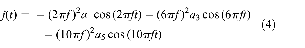
From equation (2), the acceleration and jerk functions are then derived as,

\begin{matrix} a (t) = - 2 π f a_{1} \sin (2 π ft) - 6 π f a_{3} \sin (6 π ft) \\ - 10 π f a_{5} \sin (10 π ft) \end{matrix}

(3)

\begin{matrix} j (t) = - (2 π f)^{2} a_{1} \cos (2 π ft) - (6 π f)^{2} a_{3} \cos (6 π ft) \\ - (10 π f)^{2} a_{5} \cos (10 π ft) \end{matrix}

(4)

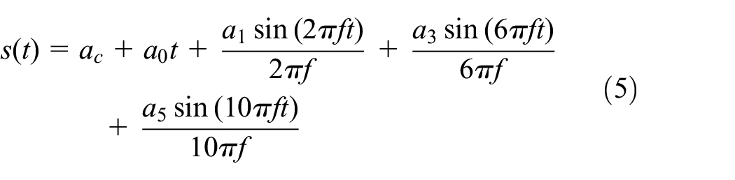
By integrating equation (2) with respect to the time t, the displacement function is derived as,

\begin{matrix} s (t) = a_{c} + a_{0} t + \frac{a_{1} \sin (2 π ft)}{2 π f} + \frac{a_{3} \sin (6 π ft)}{6 π f} \\ + \frac{a_{5} \sin (10 π ft)}{10 π f} \end{matrix}

(5)

Transition schema construction

Figure 1 shows the flow diagram of the developed transition schema. The transition schema construction includes five modules: an initialization module; a boundary conditions definition module; a motion profile constraint definition module; the contour error constraint definition module; and a trajectory parameters calculation module. The above modules are described in more detail in the following sections.

Figure 1.

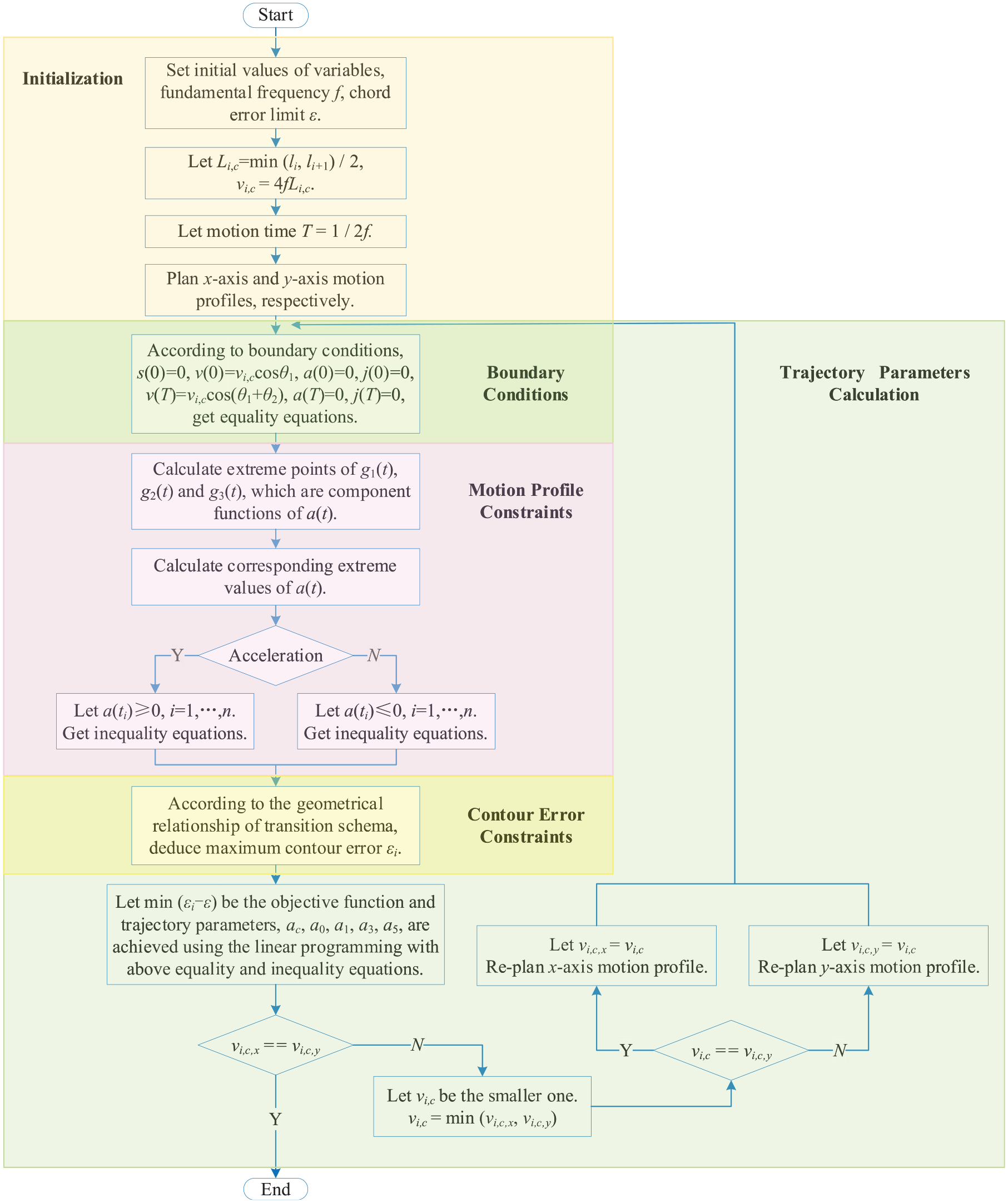
Flow diagram of the developed transition schema.

Initialization module

Figure 2 presents the proposed transition schema. In Figure 2, let the point P_i_,s be the origin to establish the x–y coordinate system and lengths of line-segments P_i₋₁P_i and P_iP_i₊₁ be l_i and l_i₊₁, respectively. The two line-segments P_i₋₁P_i and P_iP_i₊₁ form a corner, with θ₁ indicating the angle between the vector $P_{i - 1} P_{i}$ and the positive x-axis and θ₂ indicating the angle between the vectors $P_{i - 1} P_{i}$ and $P_{i} P_{i + 1}$ . The dotted curve is the transition schema that is to be synthesized by the proposed algorithm, for which the corner length for the line-segments P_i, _sP_i and P_iP_i,e is hereinafter indicated by L_i_,c. To simplify the transition curve construction process and obtain smooth axial motion profiles as shown in Figure 3, the line-segments P_i_,_sP_i and P_iP_i,e are set to have equal lengths and equal initial and final tangential velocities of v_i_,c, accelerations of a_i_,c = 0 and jerks of j_i_,c = 0. The point P_i_,m as shown in Figure 2 is the mid-point of the transition schema.

Figure 2.

Transition schema.

Figure 3.

Smooth axial motion profiles: (a) displacement, (b) velocity, (c) acceleration, and (d) jerk.

The user is to provide the required chord error ε and the fundamental frequency f of the trajectory pattern, which must be selected such that together with its first two odd harmonics, the natural modes of vibration of the system are not excited.

Boundary conditions

From the indicated end conditions and equations (2)–(5), the following boundary conditions are obtained,

s_{x} (0) = a_{c} = 0

(6)

v_{x} (0) = a_{0} + a_{1} + a_{3} + a_{5} = v_{i, c} \cos θ_{1}

(7)

a_{x} (0) = 0

(8)

j_{x} (0) = - (2 π f)^{2} a_{1} - (6 π f)^{2} a_{3} - (10 π f)^{2} a_{5} = 0

(9)

\begin{matrix} v_{x} (T) = a_{0} + a_{1} \cos (2 π fT) + a_{3} \cos (6 π fT) \\ + a_{5} \cos (10 π fT) = v_{i, c} \cos (θ_{1} + θ_{2}) \end{matrix}

(10)

\begin{matrix} a_{x} (T) = - 2 π f a_{1} \sin (2 π fT) - 6 π f a_{3} \sin (6 π fT) \\ - 10 π f a_{5} \sin (10 π fT) = 0 \end{matrix}

(11)

\begin{matrix} j_{x} (T) = - (2 π f)^{2} a_{1} \cos (2 π fT) - (6 π f)^{2} a_{3} \cos (6 π fT) \\ - (10 π f)^{2} a_{5} \cos (10 π fT) = 0 \end{matrix}

(12)

From equations (6)–(12), it is clear that if the cycle time T is set equal to half the fundamental frequency period, that is, if $T = \frac{π}{2 π f} = \frac{1}{2 f}$ , equation (11) is then always satisfied and the required equality condition that have to be satisfied become the following:

s_{x} (0) = a_{c} = 0

(13)

v_{x} (0) = a_{0} + a_{1} + a_{3} + a_{5} = v_{i, c} \cos θ_{1}

(14)

v_{x} (T) = a_{0} - a_{1} - a_{3} - a_{5} = v_{i, c} \cos (θ_{1} + θ_{2})

(15)

j_{x} (0) = - j_{x} (T) = - a_{1} - 9 a_{3} - 25 a_{5} = 0

(16)

Motion profile constrains

To achieve the desired motion profiles shown in Figure 3, the condition a(t) ≥ 0, $t \in [0, T]$ must be guaranteed, which indicates that v(t) is a monotonically increasing function from v_s to v_e. From equation (3), it can be seen that the acceleration a(t) is a sum of three sine functions and can be expressed as,

a (t) = g_{1} (t) + g_{2} (t) + g_{3} (t)

(17)

where

g_{1} (t) = - 2 π f a_{1} \sin (2 π ft)

(18)

g_{2} (t) = - 6 π f a_{3} \sin (6 π ft)

(19)

g_{3} (t) = - 10 π f a_{5} \sin (10 π ft)

(20)

The functions g₁(t), g₂(t), and g₃(t) with arbitrary amplitudes and the resulting acceleration a(t) are plotted as shown in Figure 4. As expected, and can be seen in Figure 4, the extreme values of a(t) can only occur at one of the extreme points of the fundamental frequency function g₁(t), or the functions g₂(t) and g₃(t). This is easily seen to be the case since the functions g₂(t) and g₃(t) are the first two odd harmonics of the fundamental sinusoidal function g₁(t). Therefore, the condition, a(t) ≥ 0, $t \in [0, T]$ , can be satisfied only if a(t) ≥ 0 at all extreme points of g₁(t), g₂(t), and g₃(t).

Figure 4.

Acceleration component profiles.

The extreme points of the functions g₁(t), g₂(t), and g₃(t) may be calculated as follows:

As an example, for the function g₁(t), the extreme of this sin(j) function occurs at j = (2k + 1)π/2, $k \in Z$ , where Z is the set of all integers. Then from equation (18), the extreme point equation of g₁(t) are at,

2 π ft = \frac{2 k + 1}{2} π, k \in Z

(21)

Therefore, from equation (18) for the time $t \in [0, T]$ , k is limited to,

- \frac{1}{2} \leq k \leq \frac{1}{2}, k \in Z

(22)

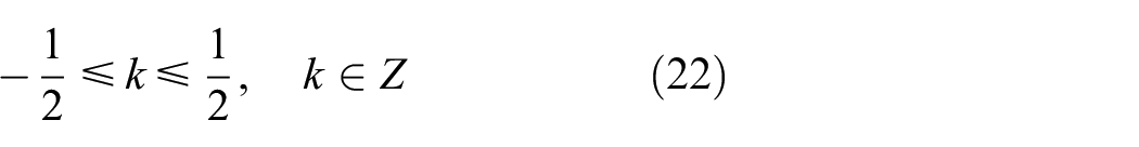
Then in general, for all integers k satisfying equation (22), the extreme point times are determined for the function from equation (21). For the case of the g₁(t), the extreme point is readily seen to be at,

t = \frac{1}{4 f}

(23)

For the functions g₂(t) and g₃(t), the extreme point times are similarly determined to be at (see Figure 4),

\begin{matrix} t_{1} = \frac{1}{20 f}, t_{2} = \frac{1}{12 f}, t_{3} = \frac{3}{20 f}, t_{4} = \frac{1}{4 f}, t_{5} = \frac{7}{20 f}, \\ t_{6} = \frac{5}{12 f}, t_{7} = \frac{9}{20 f} \end{matrix}

(24)

Now due to symmetry of the functions about t = T/2, to achieve the desired condition of a(t) ≥ 0, $t \in [0, T]$ for the synthesized motion profiles, the trajectory pattern parameters must be calculated such that the following inequality conditions are satisfies,

a (t_{i}) \geq 0, i = 1, 2, 3, 4

(25)

Contour error constraints

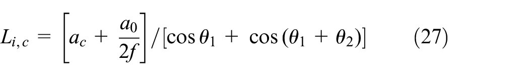
To control machining accuracy, the chord error should be bounded. In Figure 2, the transition schema is seen to be symmetric about the bisector of the angle $∠ P_{i - 1} P_{i} P_{i + 1}$ since the initial and final tangential velocities, accelerations, and jerks are the same. The distance between the points P_i and P_i_,m is therefore the contour error maximum ε_i. The computing process of the maximum is as followed:

For the corner motion displacement during the period T, from Figure 2, the corner length L_i_,c and the displacement s_x(T), equation (5), are expressed as,

\begin{matrix} L_{i, c} [\cos θ_{1} + \cos (θ_{1} + θ_{2})] = s_{x} (T) \\ = a_{c} + a_{0} T + \frac{a_{1} \sin (2 π fT)}{2 π f} + \frac{a_{3} \sin (6 π fT)}{6 π f} \\ + \frac{a_{5} \sin (10 π fT)}{10 π f} = a_{c} + \frac{a_{0}}{2 f} \end{matrix}

(26)

The corner length L_i_,c is then determined from equation (26) as,

L_{i, c} = [a_{c} + \frac{a_{0}}{2 f}] / [\cos θ_{1} + \cos (θ_{1} + θ_{2})]

(27)

The projection of corner error ε_i on the x-axis is seen in Figure 2 to be,

ε_{i, x} = ε_{i} \cos (\frac{π}{2} + θ_{1} + \frac{θ_{2}}{2})

(28)

The x coordinate of the point P_i is also seen to be,

x_{i} = L_{i, c} \cos θ_{1}

(29)

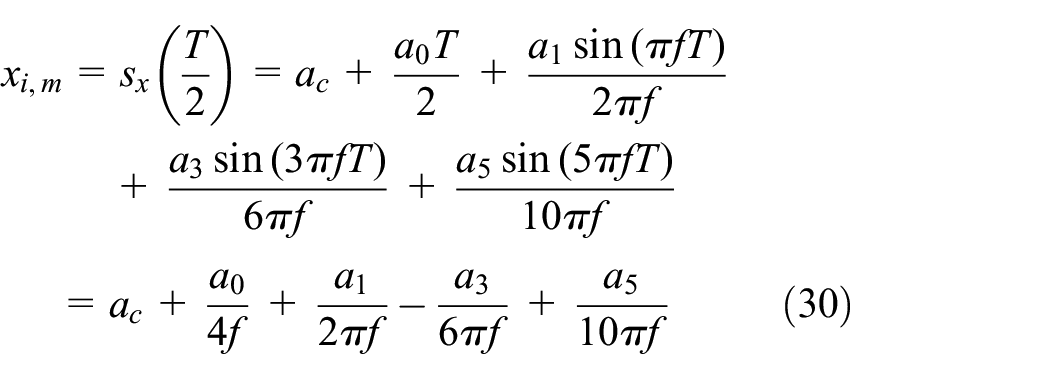
From equation (5) at the time t = T/2, the x coordinate of the point P_i_,m is,

\begin{matrix} x_{i, m} = s_{x} (\frac{T}{2}) = a_{c} + \frac{a_{0} T}{2} + \frac{a_{1} \sin (π fT)}{2 π f} \\ + \frac{a_{3} \sin (3 π fT)}{6 π f} + \frac{a_{5} \sin (5 π fT)}{10 π f} \\ = a_{c} + \frac{a_{0}}{4 f} + \frac{a_{1}}{2 π f} - \frac{a_{3}}{6 π f} + \frac{a_{5}}{10 π f} \end{matrix}

(30)

As can be seen in Figure 2, the x-axis contour error ε_i,x is,

ε_{i, x} = x_{i, m} - x_{i}

(31)

Substitute equations (27)–(30) into equation (31), the maximum chord error ε_i is obtained as,

ε_{i} = [a_{c} r_{1} + \frac{a_{0}}{4 f} r_{2} + \frac{a_{1}}{2 π f} - \frac{a_{3}}{6 π f} + \frac{a_{5}}{10 π f}] / r_{3}

(32)

where

r_{1} = \frac{\cos (θ_{1} + θ_{2})}{\cos (θ_{1} + θ_{2}) + \cos θ_{1}}

(33)

r_{2} = \frac{\cos (θ_{1} + θ_{2}) - \cos θ_{1}}{\cos (θ_{1} + θ_{2}) + \cos θ_{1}}

(34)

r_{3} = \cos (\frac{π}{2} + θ_{1} + \frac{θ_{2}}{2})

(35)

To control the machining accuracy, we should guarantee 0 ≤ ε_i ≤ ε.

Trajectory parameters calculation

To calculate the trajectory parameters for the x-axis motion profiles, the initial corner velocity v_i_,c is set at its desired value. From equations (14) and (15), the trajectory parameter a₀ is then derived as,

a_{0} = v_{i, c} [\cos θ_{1} + \cos (θ_{1} + θ_{2})] / 2

(36)

Substitute equations (13) and (36) into equation (27), the corner velocity v_i_,c in terms of the corner length L_i_,c is given as,

v_{i, c} = 4 f L_{i, c}

(37)

Now let L_i_,c be defined as the shorter of half the lengths of the line-segments P_i₋₁P_i and P_iP_i₊₁, that is, l_i and l_i₊₁, respectively, as,

L_{i, c} = min (\frac{l_{i}}{2}, \frac{l_{i + 1}}{2})

(38)

Substituting equation (38) into equation (37), the initial velocity v_i_,c is then calculated.

It is noted that the boundary conditions, equations (13)–(16); motion profile constraints, equation (25); and the contour error constrain, equation (32), are all linear functions of the trajectory parameters a_c, a₀, a₁, a₃, and a₅. Thus, their optimal values can be calculated using linear programming. The linear programming problem for determining optimal trajectory parameters to achieve minimum chord error ε_i becomes,

min (ε_{i} - ε)

(39)

subject to : {\begin{matrix} a_{c} = 0 \\ a_{0} + a_{1} + a_{3} + a_{5} = v_{i, c} \cos θ_{1} \\ a_{0} - a_{1} - a_{3} - a_{5} = v_{i, c} \cos (θ_{1} + θ_{2}) \\ - a_{1} - 9 a_{3} - 25 a_{5} = 0 \end{matrix}

(40)

{\begin{matrix} a (t_{i}) \geq 0, i = 1, 2, 3, 4 \\ ε \geq ε_{i} \geq 0 \end{matrix}

(41)

If the motion is in a deceleration phase, then the acceleration constraint becomes a(t) ≤ 0, $t \in [0, T]$ . For the y-axis, its trajectory parameters are computed by replacing cosθ₁, cos(θ₁ + θ₂), and cos(π/2 + θ₁ + θ₂/2) with sinθ₁, sin(θ₁ + θ₂) and sin(π/2 + θ₁ + θ₂/2), respectively, in equations (6)–(41).

To synchronize the corner motion, the x-axis and y-axis motion trajectories should be constructed with the same corner velocity v_i_,c. The process can be as follows:

Step 1. Assume that v_i_,c,x, v_i_,c,y are corner velocities computed by the described x-axis and y-axis trajectory synthesis process, respectively. Let v_i_,c be the smaller one of v_i_,c,x and v_i_,c,y as,

v_{i, c} = min (v_{i, c, x}, v_{i, c, y})

(42)

Step 2. If v_i_,c,x is the minimum, use the process described in the Section 2.2 and recalculate they-axis trajectory parameters with v_i_,c. If v_i_,c,y is the minimum, similarly recalculate the x-axis trajectory parameters with v_i_,c.

Step 3. By substituting the calculated trajectory parameters in equations (2)–(5), the synthesized trajectories are obtained. As can be seen, the trajectory velocity, acceleration, and jerk only contain sinusoidal functions with the selected fundamental frequency and its first two odd functions. As a result, by the proper selection of the fundamental frequency, excitation of the natural modes of vibration of the system is avoided.

Simulation validations

In this section, to demonstrate the effectiveness and performance of the proposed corner smoothing algorithm, the results of performed simulations on a typical selected system is presented and compared with results that would be obtained with one of the commonly used trajectory synthesis algorithms. Both algorithms were implemented in Visual Studio 2013 and MATLAB 2015 was used for plotting the results. The following typical settings were used: a fundamental frequency of f = 16 Hz, a sampling period of T = 2 ms, a chord error limit of ε = 0.1 mm, a programmed feedrate of F = 100 mm/s, acceleration limits of the drive axes Ax_max = Ay_max = 2000 mm/s², and jerk limits of the drive axes J_{x_}_max = J_{y_}_max = 100,000 mm/s³.

Case one

To evaluate the proposed algorithm, a jerk-limited algorithm,¹³ which constructs the transition schema and jerk-limited axial kinematic profiles in one step, is used as the comparison algorithm. As shown in Figure 5, a simple pattern with one acute angle is indicated as the desired tool path. The synthesized transition curves by applying the two algorithms are plotted. The cycle time with the proposed algorithm was calculated to be 0.0313 s, which is 9.5% faster than the jerk-limited algorithm of 0.0346 s. Figure 6(a) shows that neither algorithm exceeds the specified chord error limit ε. From Figures 5 and 6(b) to (f), we can see that the tangential and axial displacement and velocity profiles are all smooth. From Figure 6(g) to (i), it is observed that the tangential acceleration profiles of both algorithms are smooth, while the axial acceleration profiles of the comparison algorithm only have G0 continuity. In addition, since the comparison algorithm constructs axial kinematic profiles under axial acceleration and jerk limits, its jerk profiles exhibit sudden changes as shown in Figure 6(j) to (l). Noting that since such unsmooth acceleration and jerk profiles cannot be realized in the feed drive systems, the synthesized trajectories would most likely excite natural modes of vibration of the system. The proposed algorithm, however, has smooth tangential and axial velocity, acceleration, and jerk profiles, as shown in Figure 6, which the feed drive system should be capable of realizing without exciting natural modes of vibration of the system. The proposed algorithm should, therefore, achieve significantly better machining quality.

Figure 5.

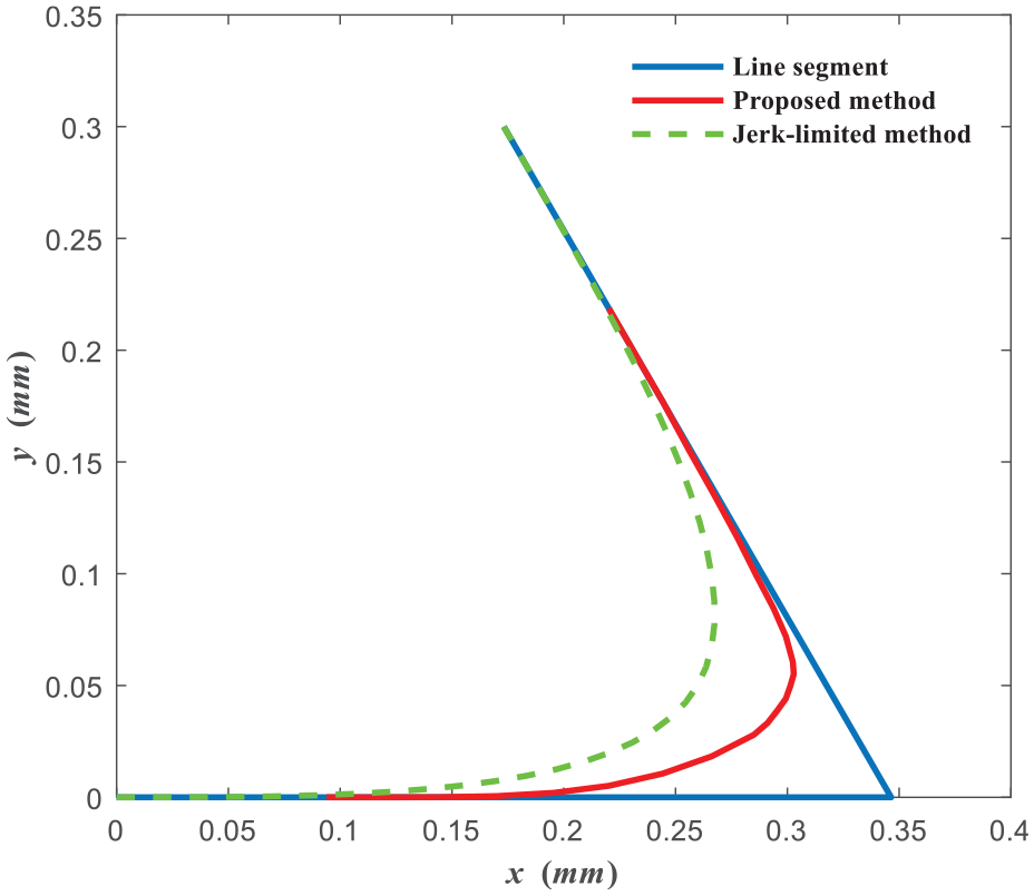
Tool path and synthesized trajectories.

Figure 6.

Comparison of the kinematic profiles for the Case one: (a) contour error, (b) x-axis displacement, (c) y-axis displacement, (d) tangential velocity, (e) x-axis velocity, (f) y-axis velocity, (g) tangential acceleration, (h) x-axis acceleration, (i) y-axis acceleration, (j) tangential jerk, (k) x-axis jerk, and (l) y-axis jerk.

To evaluate the proposed algorithm further, frequency spectrum distribution of the synthesized axial kinematic profiles is studied using Fourier integration. In the plots of Figure 7, it can be seen that the x-axis and y-axis displacements, velocities, accelerations, and jerks of the trajectories synthesized using the aforementioned jerk-limited algorithm contain a considerable number of high harmonic components, that is, harmonics with frequencies above the second odd harmonic of the fundamental frequency of the trajectory pattern. As a result, the related actuating forces/torques require producing high frequency components, which for high speed motions would in general be beyond their dynamic response and could excite natural modes of vibration of the system. As expected, Figure 7, the velocity, acceleration, and jerk profiles of the synthesized trajectory with the proposed algorithm only include the fundamental frequency and its first two odd harmonics.

Figure 7.

Comparison of the Fourier analysis for the Case one: (a) x-axis displacement of the jerk-limited algorithm, (b) x-axis displacement of the proposed algorithm, (c) y-axis displacement of the jerk-limited algorithm, (d) y-axis displacement of the proposed algorithm, (e) x-axis velocity of the jerk-limited algorithm, (f) x-axis velocity of the proposed algorithm, (g) y-axis velocity of the jerk-limited algorithm, (h) y-axis velocity of the proposed algorithm, (i) x-axis acceleration of the jerk-limited algorithm, (j) x-axis acceleration of the proposed algorithm, (k) y-axis acceleration of the jerk-limited algorithm, (l) y-axis acceleration of the proposed algorithm, (m) x-axis jerk of the jerk-limited algorithm, (n) x-axis jerk of the proposed algorithm, (o) y-axis jerk of the jerk-limited algorithm, and (p) y-axis jerk of the proposed algorithm.

To explain how trajectories with high harmonic components affect vibration of the machine tool, an undamped, 1-DOF, linear spring-mass system modeling the behavior of a vibration isolation system shown in Figure 8(a) is selected. Let the spring have a spring rate and free length of k and l, respectively. The mass of the block is m. The displacements of the mass and the system from their initial position are u and d, respectively. From the Newton’s second law, the system equation of motion is seen to be,

mu ″ = - k (u - d - l)

(43)

Figure 8.

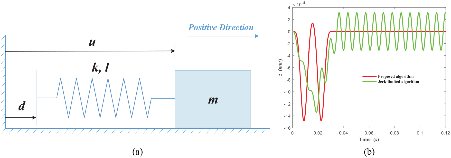
(a) Mass-spring system and (b) its vibrations.

Let $z = u - d - l, z ″ = u ″ - d ″$ , and set the natural frequency of the spring-mass system as

f_{n} = \frac{1}{2 π} \sqrt{\frac{k}{m}} = 144 Hz

(44)

Then, equation (43) can be rewritten as,

z ″ = - {(2 π f_{n})}^{2} z - d ″

(45)

Now as an example, take the y-axis motion profiles calculated using the aforementioned two algorithms as input to the dynamic system described by equation (45). The input motion d(t) is then y-axis acceleration profile, that is, $d ″ = a_{y} (t)$ .

Substituting $d ″ = a_{y} (t)$ into equation (45) and solving the resulting second order ordinary differential equation, the vibrational motion of the mass m of the spring-mass system of Figure 8(a) is determined.

As can be seen in Figure 8(b), the displacement z, which indicated the tool displacement, of the proposed algorithm is smoother than that of the jerk-limited algorithm. In addition, when the y-axis motion ends, the mass m comes to a stop with the proposed algorithm, while the mass of the jerk-limited algorithm continues to vibrate with its natural mode. It is noted that the trajectories synthesized using the jerk-limited algorithm contain a significant number of high harmonic content, which would in general cause excitation of the system modes of vibration irrespective of their frequencies. The synthesized trajectories of the proposed algorithm, however, only contain the selected fundamental frequency and two of its odd harmonics in its velocity, acceleration, and jerk terms (and even in their higher order derivatives), which would minimize the number of high harmonic components in the required actuation forces/torques. The fundamental frequency of the trajectory pattern can also be selected to avoid natural modes of vibration of the system. As a result, the system should be capable of operating with minimal vibration and achieve higher quality machining.

Case two

In this Case, a polynomial algorithm,⁴ a jerk-limited algorithm,¹³ and a jounce-limited algorithm¹⁴ are implemented as the basis for comparison with the proposed Trajectory Pattern Method (TPM) based algorithm. The polynomial algorithm constructs the transition schema with the quintic polynomial in arc length domain, then achieves tangential kinematic profiles by using a traditional tangential trigonometric velocity scheduling method. The jerk-limited algorithm uses a jerk-limited velocity scheduling method to obtain the transition schema and jerk-limited axial kinematic profiles in one step in time domain. The jounce-limited algorithm utilized a jounce-limited velocity scheduling method to construct smoother acceleration transition profiles, which can reach G3 continuity. The proposed algorithm adopts the TPM to get the transition schema and jerk-smooth axial kinematic profiles in one step in time domain as described in Section 2.

The simulation conditions of this Case are the same as those of the Case one. Figure 9(a) shows the trident-shaped pattern that is selected as the tool path. The synthesized corner tool paths with the above three algorithms are shown in Figure 9(b).

Figure 9.

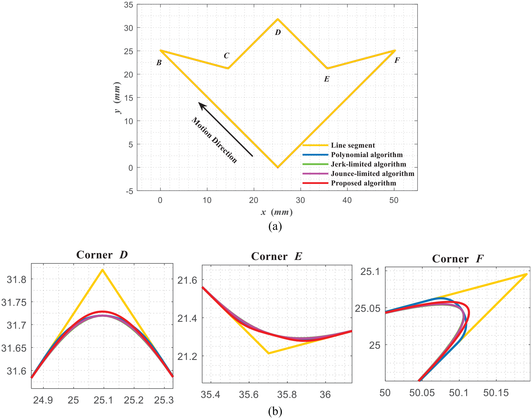
(a) Trident-shaped tool path and (b) enlarged corners.

The comparison of the simulation results is demonstrated in the plots of Figure 10. Figure 10(a) shows that tangential velocities of the four algorithms, which are all smooth and do not exceed the programmed feedrate F. As shown in Figure 10(b) and (c), axial velocity profiles of the jerk-limited, jounce-limited, and proposed algorithms are smooth and similar, while those of the polynomial algorithm is not smooth at the corners. In addition, Figure 10(d) to (g) show that axial acceleration and jerk profiles of the polynomial algorithm exceed specified limitations and fluctuate frequently around corners since this algorithm does not use an axial velocity planning method, but a traditional tangential velocity scheduling method. In the case of jerk-limited algorithm, its axial acceleration profiles are also not smooth and its axial jerk profiles exhibits sudden changes at the beginning and end of acceleration or deceleration periods around the corners. These fluctuations and sudden changes cannot be realized in the feed drive system, which makes the machining process prone to vibration.

Figure 10.

Comparison of kinematic profiles for Case two: (a) tangential velocity, (b) x-axis velocity, (c) y-axis velocity, (d) x-axis acceleration, (e) y-axis acceleration, (f) x-axis jerk, and (g) y-axis jerk.

As can be seen in the plots of Figure 10, in contrast to polynomial, jerk-limited, and jounce-limited algorithms, the proposed algorithm has smooth axial velocity, acceleration, and jerk profiles, which should make it achievable by the drive systems of the machinery system.

Fourier analysis results of the axial acceleration profiles of the four algorithms showing their frequency contents are shown in Figure 11. As can be seen in the plots of Figure 11(a) to (c) and (e) to (g) for the polynomial, jerk-limited and jounce-limited algorithms, respectively, the axial acceleration profiles of these three algorithms contain a large number of high frequency components since their trajectories are synthesized by polynomial basis curves. The trajectories of the proposed algorithm, however, are constructed with only three harmonic functions, a fundamental frequency sinusoidal function and its first two odd harmonics, in the present simulations with a fundamental frequency of 16 Hz and the first two odd harmonic frequencies of 48 and 80 Hz. The plots of (c) and (f) of Figure 11 also shows that the maximum axial acceleration frequency for synthesized trajectory with the proposed algorithm is 80 Hz, which should minimize the number of high harmonic components in the required actuation forces/torques and minimize the excitation of the system modes of vibrations. The proposed algorithm should, therefore, yield a significantly better machining quality and flexibility.

Figure 11.

Comparison of frequency distribution for Case two: (a) x-axis acceleration profile of polynomial algorithm, (b) x-axis acceleration profile of jerk-limited algorithm, (c) x-axis acceleration profile of jounce-limited algorithm, (d) x-axis acceleration profile of proposed algorithm, (e) y-axis acceleration profile of polynomial algorithm, (f) y-axis acceleration profile of jerk-limited algorithm, (g) y-axis acceleration profile of jounce-limited algorithm, and (h) y-axis acceleration profile of proposed algorithm.

The calculated computing and machining times and contour errors for the polynomial, jerk-limited, jounce-limited, and proposed algorithms are presented in Table 1. The results show that the computing time cost for the polynomial algorithm is almost twice that of the jerk-limited, jounce-limited, and proposed algorithms. It can also be seen that the machining time spent by the proposed algorithm is the shortest (1.7203 s), which is 4.7%, 1.8%, and 5.3% shorter than the jounce-limited (1.8058 s), jerk-limited (1.7515 s), and polynomial (1.8165 s) algorithms, respectively. The reason for the proposed algorithm providing the shortest machining time is due to the use of an axial velocity planning method and since no limit on the axial jerk maximum. It can, therefore, be concluded that the proposed algorithm is near time-optimal and satisfy the requirement of real-time machining, while yielding a significantly better machining quality.

Table 1.

Comparison of computing and machining times and contour error.

Algorithm	Computing time (s)	Machining time (s)	Contour error (mm)
			Max	Mean
Polynomial	0.7836	1.8165	0.0870	0.0023
Jerk-limited	0.4253	1.7515	0.0749	0.0019
Jounce-limited	0.4505	1.8058	0.0747	0.0020
Proposed	0.4742	1.7203	0.0740	0.0017

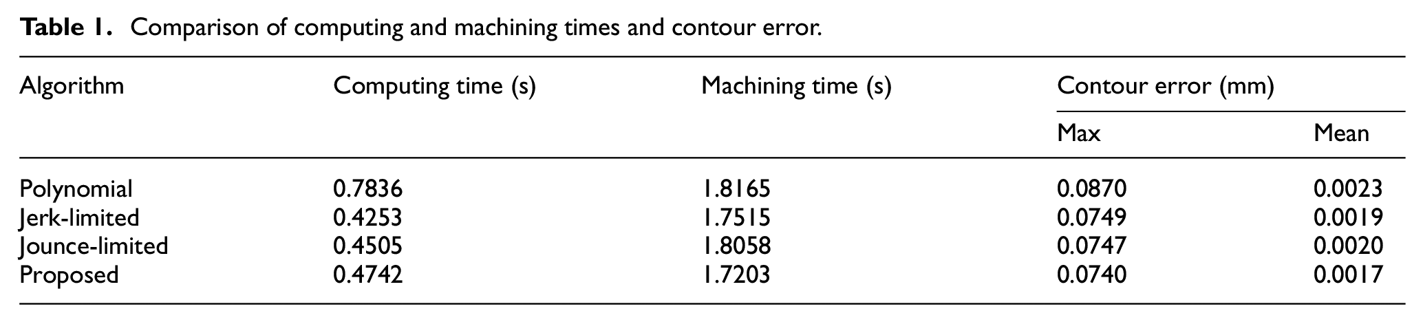
Figure 12 shows that none of the four algorithms exceeds the prescribed chord error ε, and that the maximum always happens around the corners. As can be seen in Table 1, the contour error maximum for the proposed algorithm is 0.0740 mm, which is 0.9%, 1.2%, and 14.9% lower than those of the jounce-limited, jerk-limited and polynomial algorithms, respectively. In addition, compared with the other three algorithms, the average contour error for the proposed algorithm is also smaller, that is, it is 0.0017 mm as compared to 0.0023 mm for the polynomial, 0.0019 mm for the jerk-limited, and 0.0020 mm for the jounce-limited algorithms. The proposed algorithm can, therefore, better satisfy machining accuracy requirements, while yielding a significantly better machining quality.

Figure 12.

Contour errors.

Conclusions

In this paper, a corner smoothing algorithm using the Trajectory Pattern Method (TPM) for high-speed and high-quality machining is proposed. In this algorithm, the transition schema and axial kinematic profiles are constructed simultaneously with a fundamental frequency sinusoidal function and its first two odd harmonics in time domain.

In comparison with previously published algorithms, the proposed algorithm has the following advantages: (I) the transition schema and axial kinematic profiles are constructed with a sinusoidal function with a selected fundamental frequency in one step, which reduces the smoothing process time, while avoiding excitation of the natural modes of vibration of the machinery system; (II) all velocity, acceleration, and jerk profiles are expressed by a sinusoidal function consisting of a selected frequency harmonic and its first two odd harmonics, which minimizes the number of high frequency harmonic components in the required actuation forces/torques, reducing their dynamic response requirements, and by proper selection of the trajectory fundamental frequency, the excitation of the system modes of vibration is minimized; (III) the proposed algorithm can realize smooth axial kinematic control action under chord error and dynamic response limitations of the axial drives, noting that for high-speed and high-quality machining, smooth axial kinematic profiles are more important than smooth tangential kinematic profiles; and (IV) the proposed algorithm is near time-optimal and can significantly improve machining efficiency and quality.

Since the proposed algorithm is a general corner smoothing method, it could be extended to five-axis machines and its machining efficiency and quality would be improved more significantly. However, compared to the three-axis machine, there are mainly two challenges for a five-axis corner smooth algorithm. First, the tool tip position and tool orientation need to be smoothed and synchronized. Second, due to the non-linear relationship between tool orientation vectors and rotary axis coordinates, the smooth motion of the rotary axis is not capable of being guaranteed by the smooth process of tool orientation vectors. Especially when tool orientation vectors approach singular points, fierce vibrations of the rotary axis would cause the servo alarm, even damage machine parts. Efforts should be, therefore, made to obtain smooth motion of rotary axes under the tool orientation deviation limitation in the five-axis tool center point interpolation processing.

Future work will focus on two aspects. First, we are in the process of implementing the proposed algorithm and more comparison algorithms on an open-source CNC system to analyze the performance further. Second, more limitation conditions will be considered in the proposed algorithm. We plan to publish the results shortly after.

Footnotes

Handling Editor: James Baldwin

Declaration of conflicting interests

The author(s) declared no potential conflicts of interest with respect to the research, authorship, and/or publication of this article.

Funding

The author(s) disclosed receipt of the following financial support for the research, authorship, and/or publication of this article: This work was supported by the Scientific Research Startup Foundation for High-level Talents of Nanjing Institute of Technology (Grant No. YKJ2019112), the Natural Science Foundation of Jiangsu Provincial of China (Grant No. BK20181024), and the Shuangchuang Doctoral Project of Jiangsu Province.

ORCID iDs

Hao Li

Zhuwen Yan

References

Hendrawan

Simba

Uchiyama

. Iterative learning contouring controller based on trajectory generation with linearly interpolated contour error estimation and Bézier reposition trajectory for computerized numerical control machine tool feed drive systems. Adv Mech Eng 2019; 11: 1–15.

Sun

Wang

, et al. A smooth tool path generation and real-time interpolation algorithm based on B-spline curves. Adv Mech Eng 2018; 10: 1–14.

Zhang

Yang

, et al. Study on the method of increasing turning velocity during CNC continuous machining. Manuf Technol Mach Tool 2008; 7: 79–83.

Zhang

Yang

, et al. Corner curve transition interpolation algorithm for high speed machining of micro-line segment. J Mech Eng 2010; 46: 183–191.

Ernesto

Farouki

. High-speed cornering by CNC machines under prescribed bounds on axis accelerations and toolpath contour error. Int J Adv Manuf Technol 2012; 58: 327–338.

Huang

Zhu

. A locally optimal transition method with analytical calculation of transition length for computer numerical control machining of short line segments. Proc IMechE, Part B: J Engineering Manufacture 2018; 232: 2409–2419.

Shi

Wang

, et al. Development of real-time look-ahead methodology based on Quintic PH curve with G² continuity for high-speed machining. Appl Mech Mater 2013; 464: 258–264.

Shi

Zhu

, et al. Corner rounding of linear five-axis tool path by dual PH curves blending. Int J Mach Tools Manuf 2015; 88: 223–236.

Chen

Jin

, et al. A real-time C3 continuous local corner smoothing and interpolation algorithm for CNC machine tools. J Manuf Sci Eng 2019; 141: 041004.

10.

Chen

Jin

, et al. A real-time C3 continuous tool path smoothing and interpolation algorithm for five-axis machine tools. J Manuf Sci Eng 2020; 142: 1–43.

11.

Fan

Lee

Chen

. A realtime curvature-smooth interpolation scheme and motion planning for CNC machining of short line segments. Int J Mach Tools Manuf 2015; 96: 27–46.

12.

Biagiotti

Melchiorri

. FIR filters for online trajectory planning with time- and frequency-domain specifications. Control Eng Pract 2012; 20: 1385–1399.

13.

Tajima

Sencer

. Kinematic corner smoothing for high speed machine tools. Int J Mach Tools Manuf 2016; 108: 27–43.

14.

Zhang

. Acceleration smoothing algorithm based on jounce limited for corner motion in high-speed machining. Int J Adv Manuf Technol 2018; 95: 1487–1504.

15.

Rastegar

. (IEEE). A basis trajectory approach to the inverse dynamics formulation of robot manipulators. In: IEEE international conference on systems engineering, Pittsburgh, PA, 9–11 August 1990, paper no. ICSYSE1990-203158, pp.308–311. New York: IEEE.

16.

Fardanesh

Rastegar

. A new model based tracking controller for robot manipulators using the trajectory pattern inverse dynamics. In: IEEE international conference on robotics and automation, Nice, France, 12–14 May 1992, paper no. ROBOT1992-219938, pp.2152–2157. New York: IEEE.

17.

Rastegar

Mattice

, et al. Trajectory pattern method applied to a nonlinear flexible pointing system. In: American control conference, San Francisco, CA, 2–4 June 1993, paper no. ACC1993-4793148, pp.1622–1626. New York: IEEE.

18.

Rastegar

Feng

. On the minimum harmonic trajectory pattern for point-to-point motion. In: ASME international design engineering technical conferences and computers and information in engineering conference, Washington, DC, 28–31 August 2011, paper no. DETC2011-47724, pp.359–363. New York: ASME.

A corner smoothing algorithm using Trajectory Pattern Method (TPM) for high-speed and high-quality machining

Abstract

Keywords

Introduction

Low harmonic transition schema

Trajectory pattern

Transition schema construction

Initialization module

Boundary conditions

Motion profile constrains

Contour error constraints

Trajectory parameters calculation

Simulation validations

Case one

Case two

Conclusions

Footnotes

Declaration of conflicting interests

Funding

ORCID iDs

References