
Abstract
In this study, a smooth and likelihood-based collision avoidance trajectory generation approach for autonomous navigation is presented. This article focuses on local trajectory planning for polygon shaped and differential drive vehicles, which aims to avoid obstacles when moving toward the goal. Starting from the Optimization-based Collision Avoidance framework, a new warm start method is introduced, in which the Fast Likelihood-based Collision Avoidance algorithm is modified to find a coarse trajectory which maximizes the likelihood to reach the goal. The constrained optimal control problem is reformulated to improve the smoothness and efficiency. To speed up the smoothing process, an iterative bounding box adjustment method is adopted to satisfy collision avoidance constraints. The proposed Smooth Likelihood-based Collision Avoidance (SLBCA) algorithm is robust and enables real-time optimization-based trajectory planning. Finally, extensive experimental evaluations are presented in simulations and real-world environments to demonstrate the smoothness and efficiency of SLBCA.
Keywords
Introduction
There is a growing demand for autonomous systems capable of safely locomoting in tight environments with dynamic obstacles while accomplishing complicated tasks. Prominent examples include self-driving cars, unmanned aerial vehicles, domestic service robots, and automated guided vehicles. To achieve full autonomy in these applications, one of the fundamental challenges in autonomous systems is concerned with the development of trajectory planning algorithms, which generate efficient and smooth motions, under the premise of avoiding obstacles. This challenge is further amplified when considering real-world operational constraints: autonomous vehicles often carry heavy or sensitive payloads, demanding precise motion control. To meet these requirements, the trajectory planning algorithm must account for kinodynamic constraints, collision avoidance, and real-time computation. The resulting output is a smooth trajectory, which is a spatial path augmented with a velocity profile that enables precise control of the vehicle's position over time.1,2 This trajectory generation forms the foundation for accurate path-following control.
The development of such trajectory planning algorithms in autonomous systems directly depends on advances in two core technical domains: path planning (for generating collision-free geometric paths) and trajectory optimization (for refining these paths into dynamically feasible motions).3–5 A large body of work exists on the topic of path planning, which involves searching a collision-free path from a start to a goal, given a representation of the environment. Existing path planners can be categorized into two major classes. One category is graph search-based methods, such as A*, D*, and D* Lite algorithms.6,7 The other category is sampling based methods,8–10 such as Rapidly exploring Random Tree (RRT), Probabilistic Roadmap (PRM), and their variants, have demonstrated promising results to handle maps in large scales, generating paths in a relatively short amount of time. While these conventional methods typically find the minimum cost path (often the shortest path) given a deterministically known map, a critical limitation is that the shortest path may guide the vehicle through narrow pathways leaving very few choices to avoid more obstacles. To address this issue, Zhang et al. 11 proposed a novel path planning method, that is, Fast Likelihood-based Collision Avoidance (FLBCA), which employs a probabilistic representation of the environment and seeks the highest probability of successful navigation.
Trajectory optimization builds upon the initial path to enforce dynamic feasibility and optimality, as the raw paths often lack smoothness and kinodynamic consistency. Thus, optimization-based trajectory planning methods address this by refining the path to minimize objectives such as control effort, traversal time or jerk while strictly maintaining obstacle avoidance. Historically, two major approaches of trajectory optimization have been researched. One category is the path/speed decoupled method. For example, the work in Lau et al. 12 first generates a path represented by joined quintic Bezier spline segments and then computes a velocity profile with piecewise constant accelerations. Another example is the planner integrated in the Apollo Autonomous Driving Platform, 13 which decouples the collision-free trajectory planning problem into a Dual-Loop Iterative Anchoring Path Smoothing (DL-IAPS) and a Piece-wise Jerk Speed Optimization (PJSO). 14 The other category is the path/speed coupled method which simultaneously solves the path and speed optimization problem. The Timed Elastic Band (TEB) approach 15 is proposed to optimize local trajectory with respect to dynamic constraints and nonholonomic kinematics while explicitly incorporating temporal information. TEB is available as open-source C++ code and integrated into ROS. 16 Arantes et al. 17 transformed the collision avoidance MPC into a Mixed-Integer Programming (MIP) problem by approximating the polyhedral obstacles and the ego vehicle as full dimensional polygons. However, the resulting optimization problem is computationally difficult to solve when the number of nearby obstacles is large. 18 To preserve continuity and differentiability of collision avoidance constraints, Optimization-Based Collision Avoidance (OBCA)19,20 expresses the collision avoidance problem as an optimal control problem and uses strong duality of convex optimization, also belongs to the path/speed coupled method. Inspired by OBCA, He et al. 21 proposed Temporal and Dual warm starts with Reformulated OBCA (TDR-OBCA) algorithm with improved robustness, driving comfort, and efficiency. It should be noted that these approaches usually have high computation complexity.
Building upon and extending the objectives of trajectory optimization, this article aims to solve the trajectory planning problem for polygon shaped and differential drive vehicles to enable smooth and fast autonomous movement in complex environments. The proposed method draws inspiration from the well-known Nonlinear Model Predictive Control (NMPC) framework.22,23 A notable example of the NMPC framework is the OBCA, in which both vehicle dynamics and collision avoidance are elegantly incorporated into a single large-scale NMPC problem with only continuous variables by formulating the collision avoidance constraints into their dual expressions exactly.19,20 Despite OBCA's advantages, two critical issues remain unsolved. First, a warm start algorithm should be well designed since a good initial guess will improve convergence speed and final solution quality. 21 The method for obtaining a warm start is problem-dependent and should be tailored to the system at hand. For instance, the well-known A* and Hybrid A* algorithms provide good initial guesses for quadcopter trajectory planning and automated parking problem, respectively. 24 However, they are unsuitable for warm-starting the problem in this study. Second, OBCA introduces additional dual variables along with corresponding nonlinear equalities and inequalities to represent the collision avoidance constraints accurately. 20 Consequently, it often suffers from high computation complexity and may fail to meet the real-time requirements in dynamic environments.
To address these issues systematically, this article proposes a Smooth Likelihood-Based Collision Avoidance (SLBCA) algorithm. For the first issue, a modified version of Fast Likelihood-Based Collision Avoidance (FLBCA) algorithm11,25 which employs a probabilistic representation of the environment is used to generate a warm start efficiently. Specially, the modified FLBCA is used for path planning, while a pose follower computes control commands to track the planned path. The vehicle's states over a period of time are simulated based on the differential motion model and saved as an initial trajectory. Benefiting from that FLBCA maximizes the likelihood of reaching the goal, this initial trajectory also has the highest probability of successful navigation and prefers opener spaces for traversal. It is worth mentioning that FLBCA is limited to circular or near circular vehicles, whereas SLBCA extends to full-dimensional polygon vehicles.
Note that FLBCA does not incorporate the motion smoothness, so this initial trajectory should be optimized further. During the smoothing process, an iterative bounding box adjustment method is adopted to handle the second issue, namely, the high computation complexity and real-time requirements caused by OBCA's dual variables and nonlinear constraints. Unlike the exact method used in OBCA, the proposed method greatly reduces the scale of the optimization problem by eliminating dual variables and their related constraints. This allows the initial trajectory to converge quickly to a smooth, safe and dynamically feasible trajectory in real-time. Specifically, the advantages of SLBCA can be summarized as follows:
The proposed SLBCA combines the merits of FLBCA and OBCA. While FLBCA and OBCA each offer distinct advantages, their integration poses challenges. First, FLBCA's probabilistic path planning assumes circular vehicle geometry, requiring fundamental modifications to handle polygonal shapes, which is a necessity for real-world applications. Second, OBCA's exact collision avoidance formulation, though mathematically elegant, introduces dual variables that severely limit real-time performance. Crucially, these methods operate on opposing principles: FLBCA prioritizes navigation likelihood through discrete path sampling, while OBCA enforces continuous optimization with smoothness guarantees. Bridging this gap demands a novel framework that preserves FLBCA's probabilistic advantages while embedding them within OBCA's optimization structure, all without compromising computational efficiency. These challenges motivate our proposed SLBCA architecture. The architecture of SLBCA is shown in Figure 1.

SLBCA architecture. SLBCA: Smooth Likelihood-based Collision Avoidance.
In summary, the proposed SLBCA generates smooth, safe, and efficient trajectories in real-time, while maximizing the probability of successful navigation. It is worth mentioning that the proposed method can be adapted to omnidirectional vehicles or unmanned aerial vehicles easily. To the best of the authors’ knowledge, no similar work has been demonstrated previously.
The rest of this article is organized as follows. In the third section, the optimization-based trajectory planning problem for polygon shaped and differential drive vehicles is introduced. After that, the fourth section presents the SLBCA in detail. Later on, experiments in simulations and real-world environments demonstrating the efficacy of the proposed algorithm are given in the fifth section. Finally, conclusions are drawn in the sixth section.
Problem statement
In this section, the kinematics model of differential drive vehicles is first introduced and then the local trajectory planning problem is formulated as a constrained optimal control problem, similar to OBCA, TDR-OBCA.19–21
The kinematics model can be described as x’ = f (x, u). The state of the vehicle is defined as x = [X, Y, θ]T ∈ ℝ3 under the global coordinate, where X and Y are the vehicle's position and θ the angle between the forward direction of the vehicle and the horizontal axis. The input u = [v, w]T ∈ ℝ2 consists of the linear and angular command velocities. At time step k, the state and input are xk = [Xk, Yk, θk]
T
and uk = [vk, wk]
T
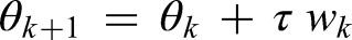
, respectively. The continuous time system can be discretized using a second-order Runge-Kutta method, given by


The local trajectory planning problem can be stated as follows. It takes the obstacles, a start state, a waypoint (or a goal) state as input and then generates a smooth obstacle-free local trajectory, which will be sent to a trajectory tracker to move toward the goal. Optimization-based approaches express the collision avoidance problem as an optimal control problem, and then it will be solved by numerical optimization techniques. The optimal control problem is to find a control sequence over a horizon K, making the vehicle to navigate from an initial state xS to a goal state xF, while minimizing the objective


Obviously, solving the problem in equation (3) is time-consuming because of its high degree of nonconvexity and nonlinearity. As is well known, it is very important to obtain a good initial guess (a warm-starting solution) because different initial guesses will lead to different local optimal solutions. In addition, the convergence rate and final solution quality will be greatly improved if a good initial guess is provided to the numerical solvers. However, computing a good initial guess is often difficult and highly problem dependent. Zhang et al. 24 demonstrate the efficacy of the OBCA methods on quadcopter navigation and automated parking problems. For quadcopter navigation, the well-known A* algorithm is used to find a path in the position space without collision with obstacles. Unfortunately, A* is not able to generate a good initial guess for the automated parking problem as it does not incorporate the vehicle's nonholonomic dynamics. To address this issue, Hybrid A*, a kinodynamic path planning algorithm, is adopted to provide an obstacle-free path for the self-driving vehicle using a simplified kinematic bicycle model. 5 And then all the warm-starting vehicle states and inputs that satisfy the system dynamics can be computed based on the Hybrid A* path.
However, A* and Hybrid A* are not suited to warm start the local trajectory planning problem for the polygon shaped and differential drive vehicle in this article. The reasons are listed as follows. Generally, A* is used to find the shortest path from start to goal if the vehicle geometry can be approximated as a circle. It may be too conservative to approximate the polygon-shaped vehicle by a circumscribed circle. Furthermore, due to the gridding, the A* path exhibits a zigzag pattern. Although the differential drive vehicle is able to move along the A* path, it has to turn on the spot at the join points of line segments frequently. Thus, the A* path is not smooth enough. Hybrid A* uses a simplified bicycle model to create candidate nodes and cannot be applied to generate the initial guess for the differential drive vehicle. Inspired by the path planning method in FLBCA, a new algorithm is proposed to generate a coarse obstacle-avoidance trajectory, providing a good warm starting for the optimal control problem in equation (3), which will be detailed in the “Simulations” and the “Real-world tests” sections.
Another key challenge in solving equation (3) is the presence of the collision-avoidance constraints
To compare with the proposed iterative method directly and apparently, the original formulation of OBCA is presented here. The optimization is performed over states


In OBCA, the vehicle geometry is modeled through the rotation and translation of an initial convex polygon
Core algorithms
In this section, the proposed SLBCA for differential drive vehicles is described. The “Modified FLBCA” section begins by introducing the modified FLBCA for path planning and then the “Coarse trajectory generation” section introduces the coarse trajectory generation approach based on the modified FLBCA. The “Iterative trajectory smoothing” section presents the iterative method to speed up solving the constrained and nonlinear optimal control problem. Finally, the “Comparative Analysis” section includes a comparison table that systematically contrasting the three methods across several critical dimensions.
Modified FLBCA
FLBCA is a path planning algorithm that maximizes the likelihood of successful navigation to the goal on the basis of a probabilistic representation of the environment. 11 The greatest advantage of FLBCA is the high efficiency as it moves the processing offline as much as possible to accelerate the online processing. FLBCA precomputes a motion primitive library and organizes it into groups. Figure 2 gives an example of seven path groups. The paths in a group split in multiple directions horizontally. As is shown in Figure 2, the path first splits in seven directions and each splits in another seven directions. As a result, each group has 49 paths. It is assumed that there are seven path groups every 10 degrees within the 360-degree range.

An example of seven path groups.
For the collision check FLBCA uses a voxel grid overlaid with sensor range and pre-establishes the correspondences between the voxels and paths, which are stored in an adjacency list. All the paths that are occluded by a voxel are labeled by only calculating the distance between the voxel and the path as the vehicle is approximated as a circle. For polygon shaped vehicles, the association will take more time because it has to check whether the vehicle collides with a voxel when it moves along the path. Fortunately, it can be computed off-line. The precomputed paths and adjacency list are loaded into the vehicle computer memory when the system starts. Therefore, FLBCA only needs to select the obstacle-free group with maximum likelihood toward the waypoint among 36*7 groups. For a complete description of the FLBCA, please refer to reference [11]
The optimal path selected by FLBCA is collision-free for circular vehicles. However, it may be unsafe for polygon-shaped vehicles. As depicted in Figure 3, θ indicates the vehicle's orientation angle measured from the horizontal axis, and φ corresponds to the initial path tangent angle relative to this axis. When the deviation between θ and φ exceeds a predetermined threshold, an in-place rotation maneuver is initiated to align the vehicle orientation with the desired path direction. To ensure safety during this maneuver, the modified FLBCA incorporates a rotation-aware collision check for polygon-shaped vehicles. Without loss of generality, a simple method for the rotation-aware collision check with a rectangular vehicle is illustrated, as is shown in Figure 3. Let α1 and α2 denote the maximum permissible clockwise and anticlockwise rotation angles of the rectangular vehicle, respectively. If the obstacle distance d1 exceeds the radius of the rectangle's circumcircle, the vehicle is collision-free. The ranges of α1 and α2 are both 0 to 360 degrees. If d1 is smaller than the radius of the rectangle's incircle, the vehicle has already collided with the obstacles. In this case, both α1 and α2 are 360 degrees. In the remaining case, that is, d1 lies between the radius of incircle and the circumcircle, α1, α2 could be computed easily. For the example given in Figure 3, the vehicle can rotate α1 degrees clockwise, and rotate α2 degrees anticlockwise. If α1 > θ – φ > 0 or –α2 < θ – φ < 0, the vehicle is safe to rotate in place.
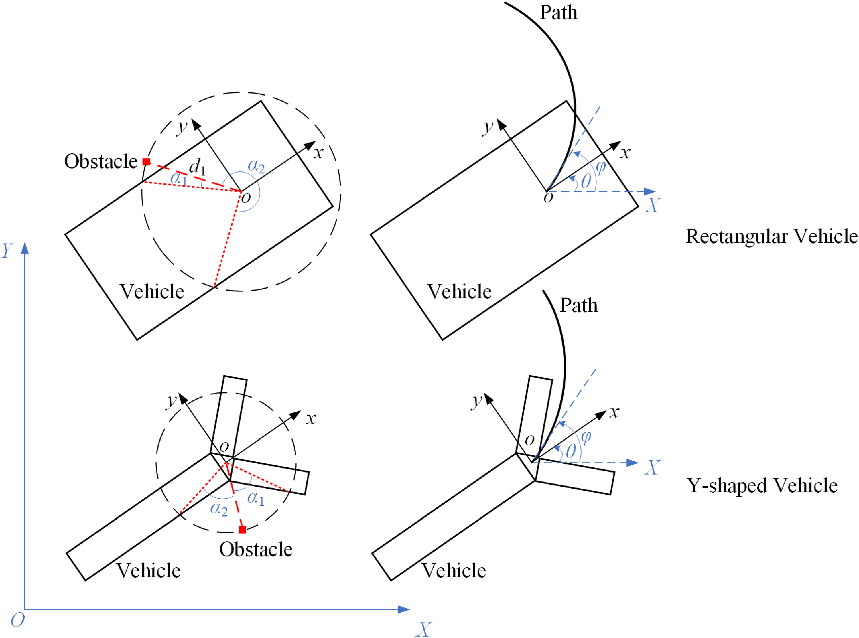
Illustration of rotation-aware collision check.
For a Y-shaped vehicle as shown in Figure 3, if the obstacle distance d1 exceeds the radius of its circumscribed circle, then in-place rotation is guaranteed to be collision-free. If d1 is less than the radius of the circumscribed circle, the maximum permissible clockwise and anticlockwise rotation angles (α₁ and α₂) can be easily determined via the geometric method shown in Figure 3. The in-place rotation is safe when either: α1 > θ – φ > 0 or –α2 < θ – φ < 0 is satisfied.
During the navigation of FLBCA, obstacles detected by perception sensors are represented as black grid points and are not inflated to maintain a safe margin. In practice, the assumed obstacle-free path may be too close to obstacles. In this article, FLBCA is used to generate the coarse trajectory as a warm start, and collision-free condition is guaranteed by bounding boxes, which will be detailed in the section “Iterative trajectory smoothing”. If the initial solution is too close to obstacles, some bounding boxes will be very small, thus the smoothness of the final trajectory will not be improved distinctly. Therefore, each obstacle is inflated by adding eight additional obstacles. Figure 4 illustrates the eight added obstacles with different inflation sizes.

Obstacle inflation with inflation size = 0, 1, 2, 3.
The modified FLBCA for path planning is presented in Algorithm 1, featuring two key improvements over the original FLBCA. First, it introduces rotation-aware collision checking to verify path safety by examining allowable rotation angles for nonoccluded candidate paths. Second, it implements adaptive obstacle inflation through a dynamic process that starts from size n and gradually reduces to 0. The algorithm terminates when either identifying a collision-free path group with maximum likelihood, in which case it returns the optimal path, or when no valid path is detected, resulting in a no-path-found output.
FLBCA avoids online search to reduce the computational complexity, enabling fast autonomous navigation in cluttered environments. Furthermore, FLBCA seeks the highest probability of successful navigation, leaving more choices for obstacle avoidance during the navigation. However, the main shortcoming is that the vehicle may not move smoothly. At each step, FLBCA merely maximizes the likelihood to successfully reach the goal in determining the immediate next step and the path group selected at each step may be unstable as the smoothness of vehicle movement is not considered. If the tangent direction at the start point of the selected path group differs much from the current orientation of the vehicle, the path follower, which controls the vehicle to move along the path as accurately as possible, will turn toward the desired direction while decelerating. Otherwise, the path follower will accelerate to the desired speed and move along the path. Therefore, the linear and angular speeds of the vehicle may vary frequently. To address this problem, the SLBCA is proposed, in which a coarse trajectory based on the modified FLBCA is generated firstly and then the coarse trajectory will be smoothed using an iterative trajectory smoothing approach, ensuring that it remains collision-free.

Coarse trajectory generation
This section presents the process of coarse trajectory generation. Given a waypoint, the movement of the vehicle can be simulated with a local path planner and a path tracking controller. The planning loop is assumed to work at a rate of 10HZ and the control frequency should be higher than the planning frequency in general, for example, 100HZ. Here, the modified FLBCA is used for path planning and the controller computes the control command to follow the planned path. The initial vehicle state and the control inputs are used to simulate the vehicle states over a period of time based on differential motion model. Finally, the simulated vehicle states

Iterative trajectory smoothing
As mentioned before, equation (4) elegantly incorporates both vehicle dynamics and obstacle avoidance into a single optimization problem, but usually incurs high computation costs. However, autonomous navigation systems require real-time local trajectory planning to account for dynamic changes. In order to speed up the trajectory smoothing process, the optimization model in OBCA is reformulated here, the dual variables 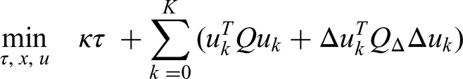


where 
With given fixed bounding boxes, equation (5) can be solved by a nonlinear numerical optimization solver. Thus, the remaining challenge is to determine proper sizes of the bounding boxes to ensure safety while not over-sacrificing the trajectory smoothness. An iterative approach is proposed. Once a local trajectory is optimized by solving equation (5), the iteration uses precise collision detection by checking the sensor data points and trajectory points one by one. It is worth mentioning that the precise shape of the vehicle is considered during the collision check. If the smoothed solution passes the collision check with all obstacles, the iteration will be terminated. Otherwise, the corresponding bounding box will be reduced. The overall algorithm is shown in Algorithm 3. The detailed procedure

of bounding box update is illustrated in Figure 5. For the smoothed trajectory at iteration i, if it collides with obstacles at time k, the corresponding state bounding box size is reduced by
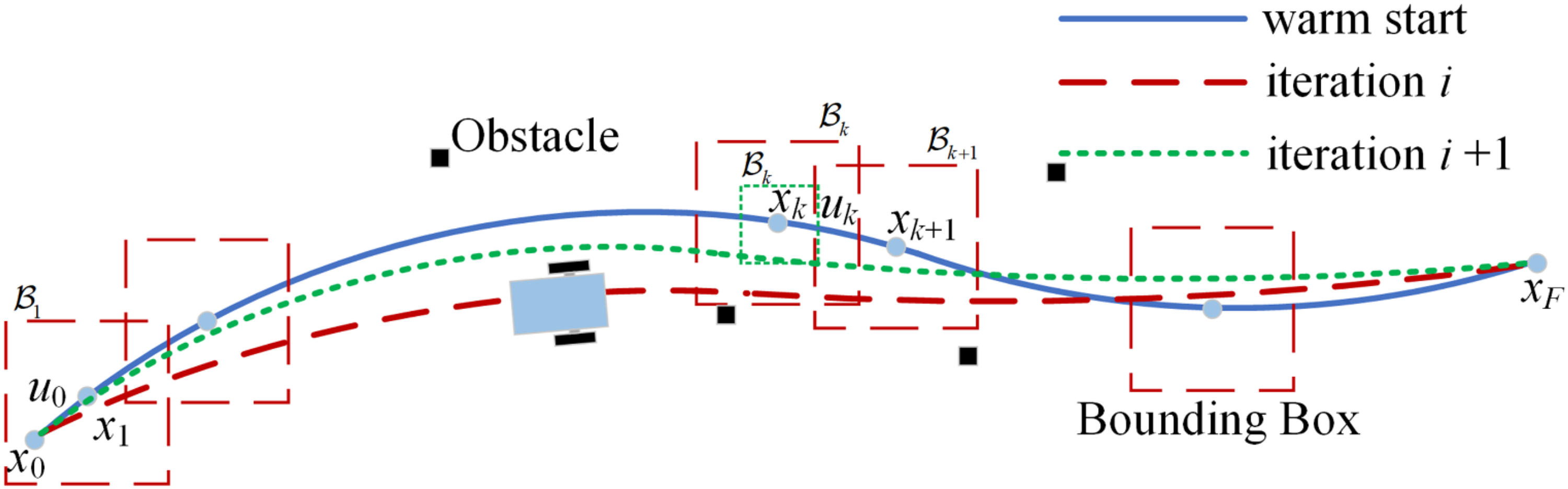
Illustration of detecting collision and updating bounding box
Comparative analysis
The proposed SLBCA combines strengths from both FLBCA and OBCA while addressing their limitations. As shown in Table 1, SLBCA inherits FLBCA's probabilistic navigation approach for warm-start generation while adopting OBCA's optimization framework for trajectory smoothing. Key innovations include: (1) extending collision checking to full polygonal shapes unlike FLBCA's circular approximation, (2) maintaining FLBCA's likelihood maximization principle within an optimization framework, and (3) replacing OBCA's computationally expensive dual formulation with iterative bounding boxes. This hybrid approach achieves real-time performance comparable to FLBCA while delivering smoothness and precision matching OBCA.
Comparative analysis of the proposed SLBCA, FLBCA, and OBCA.

FLBCA: Fast Likelihood-based Collision Avoidance; OBCA: Optimization-based Collision Avoidance; SLBCA: Smooth Likelihood-based Collision Avoidance.
Experiment results
In this section, the proposed SLBCA is validated in both simulations and real-world tests. In the simulation tests, it is demonstrated firstly that SLBCA is able to generate a coarse trajectory by the modified FLBCA and a smooth trajectory while ensuring safety by the iterative trajectory smoothing method. Next, the computation efficiency of solving equation (5), in comparison with that of equation (4) is shown. Then, SLBCA and FLBCA are compared in the same simulation environment, which proves the smoothness of SLBCA. At last, SLBCA is proved to be valid for polygon-shaped vehicles even in challenging scenarios where tight obstacle spacing restricts vehicle rotation and necessitates complex detour maneuvers. In the real-world tests, SLBCA is deployed on a real autonomous vehicle, and the smoothness and efficiency are validated in the real-world tests.
In all the simulations and real-world tests, the linear speed of the vehicle is limited between v
Simulations
The polygon-shaped vehicle is modeled as a rectangle of size 0.8 × 0.7 m and the distances from the rotation center to the front, rear, left, and right side are 0.2, 0.6, 0.35, and 0.35 m, respectively. All subsequent simulations were performed on a computer with an Intel i5-7400 processor clocked at 3.0 GHz. The simulations were implemented in C++ programming language. The problem described by equation (5) is solved with the nonlinear solver IPOPT. 29
The simulation scenario shown in Figure 6 is set to be 5.0 m wide and 10.0 m long. It is assumed that all the polygon-shaped obstacles are known in advance and converted to laser data points. As is shown in Figure 6, the coordinate origin is located at the lower left corner of the map, and the initial position of the vehicle is Xs = 2.0 and Ys = 2.0. Initially, the vehicle is standstill and oriented to the right, that is, vs = ws = θs = 0. For the end condition, the position is fixed at Xf = 8.0 and Yf = 2.0 and the orientation is not fixed, represented by a green dot in Figure 6. Given the vehicle's initial pose and the goal point, FLBCA is used for path planning and a path tracking module controls the vehicle to move along the planned path. Finally, the simulated vehicle states

The vehicle’ path corresponding to (a) the coarse trajectory generated by Algorithm 2 and (b) the smoothed trajectory obtained by Algorithm 3.

(a) Linear and (b) angular speed of the coarse and smoothed trajectory.
In order to demonstrate the computation efficiency of the proposed iterative trajectory smoothing algorithm, the computation time required for directly solving equation (4) and iteratively solving equation (5) are compared using the same warm start and IPOPT tool. The vehicle's initial pose and 25 goal positions selected on the map are shown in Figure 8(a). It can be seen from Figure 8(b) that the computation time required to directly solve equation (4) is about 20 times that of the iterative trajectory smoothing algorithm. This is not surprising since dual variables and corresponding nonlinear equalities and inequalities are not introduced to accurately represent the collision avoidance constraints, which greatly reduces the scale of the optimization problem.

(a) Selected goal positions and (b) computation time of solving (4) directly and solving (5) iteratively.
To further validate the effectiveness of SLBCA, we conducted extensive experiments in 100 randomly generated environments, performing 20 trials per environment to ensure statistical significance. Figure 9 shows an example environment. The proposed method SLBCA was compared with two state-of-the-art local trajectory planners: TEB, and Lattice Planner (LP). Figure 9 demonstrates that while TEB and LP can guide the vehicle through narrow passages, SLBCA tends to prefer open spaces even when this results in longer paths. This strategic behavior proves particularly advantageous in real-world applications where system uncertainties are unavoidable. We also tested a variant called SLBCA_c which uses circumscribed circles without rotation collision checks, and the results show it produces overly conservative paths, confirming the importance of our full collision avoidance formulation. Specifically, when vehicles attempt to navigate through narrow channels, they achieve only a 60% success rate due to various practical challenges such as localization errors and motor control inaccuracies. In contrast, when traversing through wider passages, the success rate reaches 100%. This key observation directly supports our claim that SLBCA maximizes the likelihood of successful goal attainment through its preference for safer, more open paths.

An example environment and the vehicle's actual path from each method.
FLBCA has been tested in a simulation environment, 30 in which FLBCA is used for local path planning and a pose follower is designed to control the vehicle to move along the planned path. The simulation environment is shown in Figure 10. Initially, the vehicle is standstill and starts at #4 goal point facing upwards. Then four goal points numbered #1, #2, #3, and #4 are published to the vehicle in sequence. When the vehicle is approaching the goal point and the distance between them is <0.5 m, another goal point will be published. Finally, the vehicle goes back to the start point. Figure 10(a) shows the vehicle's actual path. In the same simulation environment, the proposed SLBCA is used for local trajectory planning and a simple LQR controller is used for trajectory tracking. The vehicle's actual path is shown in Figure 10(b), which is similar to the path in Figure 10(a). The path using the FLBCA is close to obstacles. In contrast, the path using the SLBCA keeps a safe distance from the obstacles because each obstacle is inflated by adding eight additional obstacles. Furthermore, the path using the SLBCA is a bit smoother. Figure 11(a) presents the linear speed of the vehicle during the whole movement using the FLBCA and SLBCA and Figure 11(b) presents the angular speed. Obviously, the linear and angular speeds change dramatically, resulting in obvious oscillation if FLBCA is adopted. However, if the proposed SLBCA is used, the vehicle moves much more smoothly.

Vehicle's actual paths using (a) FLBCA and (b) SLBCA. FLBCA: Fast Likelihood-based Collision Avoidance; SLBCA: Smooth Likelihood-based Collision Avoidance.

(a) Linear and (b) angular speed commands using FLBCA and SLBCA in the simulation test. FLBCA: Fast Likelihood-based Collision Avoidance; SLBCA: Smooth Likelihood-based Collision Avoidance.
FLBCA can only be applied to circular or near circular vehicles as mentioned earlier. The following simulation demonstrates SLBCA's applicability to polygonal vehicles under challenging navigation conditions. We consider a rectangular vehicle (1.2 m × 0.7 m) with its rotation center at the geometric center. The vehicle is initially positioned in a tightly constrained environment between two closely spaced obstacles, a configuration that prohibits vehicle rotation and forces nonintuitive maneuvering. As shown in Figure 12, the vehicle must execute a carefully planned detour to reach the designated goal point, initially moving away from the target to circumvent the obstacles before reorienting toward the destination. Using SLBCA for local trajectory planning coupled with LQR control for trajectory tracking, the vehicle successfully navigates this challenging scenario, with the complete autonomous path execution clearly illustrated in Figure 12.

The actual path of the rectangular vehicle moving to the goal position.
Real-world tests
The proposed SLBCA is also tested in the real world with a rectangular differential drive vehicle shown in Figure 13(a). The distances from the center to the front, rear, left, and right side are 0.2, 0.6, 0.35, and 0.35 m, respectively. The vehicle is equipped with a 3D Velodyne laser scanner. A 2.8 GHz i7 embedded computer performs all onboard processing. Figure 13(b) provides an overview of the indoor test site with the start and goal points.
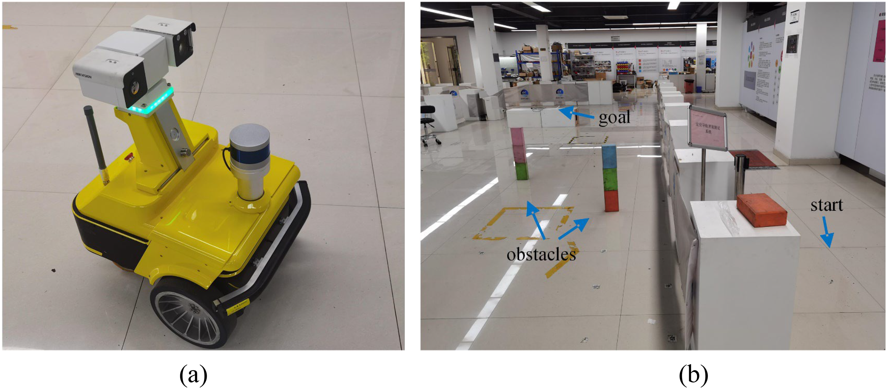
Real word test: (a) a photo of the experiment vehicle, (b) an overview of the test site with the start and goal point.
In this test, the autonomous navigation system mainly includes three parts: a global path planner, a SLBCA local trajectory planner, and a LQR tracking controller. After receiving a goal point, the global planner will generate a smooth and safe path connecting the start and goal points based on the map. With the global path, then a waypoint is chosen dynamically for the SLBCA local trajectory planning. The optimal local trajectory is passed into the LQR control module, which sends linear and angular speed commands to drive the ego vehicle following the provided trajectory. The actual path of the vehicle from start to goal is shown in Figure 14(a).

The actual path of the real vehicle using (a) SLBCA and (b) modified FLBCA. FLBCA: Fast Likelihood-based Collision Avoidance; SLBCA: Smooth Likelihood-based Collision Avoidance.
For comparison, the modified FLBCA is used for local path planning, while a pose follower is employed for path tracking. The actual path of the vehicle is given in Figure 14(b). Figure 15 shows linear and angular speed commands of the vehicle using modified FLBCA and SLBCA. It can be observed that when applying the modified FLBCA, the linear and angular speed commands oscillate noticeably, resulting in unsmooth vehicle movement. In contrast, linear and angular speed commands are much smoother with the designed SLBCA. Furthermore, the travel time of the vehicle is reduced from about 35 to 24 s.

(a) Linear and (b) angular speed commands using the modified FLBCA and SLBCA in real-world tests. FLBCA: Fast Likelihood-based Collision Avoidance; SLBCA: Smooth Likelihood-based Collision Avoidance.
Conclusion
In this article, the local trajectory planning problem for polygon shaped and differential drive vehicles is studied. SLBCA, a robust and efficient local trajectory generation algorithm for autonomous navigation in complex environments is proposed. SLBCA decouples the real-time motion planning problem as a front-end coarse trajectory generation and a back-end nonlinear trajectory optimization. As a result, the optimal trajectory generated by SLBCA is smooth and efficient, as well as maximizes the likelihood to successfully reach the goal. In order to speed up the trajectory optimization process, bounding boxes are used to ensure safety and their sizes are adjusted iteratively. In various simulations it has been shown that SLBCA is able to generate a coarse trajectory by the modified FLBCA and it can be smoothed in real-time by the iterative trajectory smoothing method. The proposed iterative method is about 10 times faster than the OBCA which solves the optimization problem directly. In addition, SLBCA proves effective for polygon shaped vehicles even in challenging conditions where tight obstacle spacing prevents vehicle rotation and requires complex detour maneuvers. The smoothness and efficiency of SLBCA have also been validated in real-world tests with a rectangular differential drive vehicle. Both in simulations and real-world tests, the vehicle moves more smoothly with SLBCA, compared to FLBCA. In addition, the real-world test shows that the efficiency is greatly improved as the travel time from start to goal is reduced from about 35 (modified FLBCA) to 24 s (SLBCA).
Supplemental Material
sj-txt-1-arx-10.1177_17298806251352007 - Supplemental material for Smooth likelihood-based collision avoidance for polygon shaped and differential drive vehicles
Supplemental material, sj-txt-1-arx-10.1177_17298806251352007 for Smooth likelihood-based collision avoidance for polygon shaped and differential drive vehicles by Yang Zhou and Linjie Kong in International Journal of Advanced Robotic Systems
Supplemental Material
Supplemental Material
Supplemental Material
Supplemental Material
Footnotes
Author contributions
YZ conceived and designed the study. YZ and LK developed the algorithm and performed the simulations and experiments. LK drafted the manuscript. YZ helped organized the manuscript.
Funding
The authors disclosed receipt of the following financial support for the research, authorship, and/or publication of this article: This work was supported by Zhejiang Provincial Department of Education Research Project under Grant [number Y202352455], and the Key Research Project of ZUME under Grant [number VU24B01].
Declaration of conflicting interests
The authors declared no potential conflicts of interest with respect to the research, authorship, and/or publication of this article.
Supplemental material
Supplemental material for this article is available online.
References
Supplementary Material
Please find the following supplemental material available below.
For Open Access articles published under a Creative Commons License, all supplemental material carries the same license as the article it is associated with.
For non-Open Access articles published, all supplemental material carries a non-exclusive license, and permission requests for re-use of supplemental material or any part of supplemental material shall be sent directly to the copyright owner as specified in the copyright notice associated with the article.