Sage Journals: Discover world-class research

Abstract

Due to edge feature defects of markers, the visual measurements for the servo control of planar manipulators often exhibit systematically distributed errors even after conventional distortion correction and camera calibration. Then, the measurement errors of visual servo system have strongly limited the absolute positioning accuracy for the feedback control of the planar manipulators. In this paper, a monocular visual measurement error prediction and feedback control method is proposed for a planar manipulator. First, the monocular vision captures markers and extracts pixel information regarding the manipulator's endpoint, while the data from the laser tracker is converted into the same coordinate system to compare and compensate the visual measurement errors. Second, the visual measurement errors of the entire workspace are obtained using visual measurement error prediction based on radial basis function neural network spatial interpolation. The measurement accuracy of the visual measurement system was improved by 91.1%. Finally, the visual measurement error prediction-based feedback controls are conducted for the positioning of planar manipulator. The experiments demonstrate that the positioning accuracy of the planar manipulator is significantly improved via the applications of the proposed method. Its positioning accuracy can reach ±0.2 mm.

Keywords

Planar manipulator visual measurement accuracy monocular vision RBF neural network

Introduction

The absolute positioning accuracy of the manipulator is one of the main indicators reflecting the performance of the manipulator, which can be improved by calibrating the positioning error of the end position of the manipulator. The absolute positioning accuracy of industrial manipulator can only reach about ±0.2 mm.¹ The primary measurement tools for planar manipulators include laser trackers and vision measurement systems, each offering different levels of accuracy.² Laser trackers offer micrometer-level measurement accuracy, rendering them ideal for applications demanding ultrahigh-precision positioning. However, their implementation presents principal disadvantage: (1) cost-prohibitive acquisition expenses, typically ranging from hundreds of thousands to millions of USD; (2) substantial physical footprint hindering rapid field deployment; (3) restricted software customization capabilities in commercial systems, particularly the inability to perform real-time manipulator motion monitoring due to inherent offline measurement architectures.³ The cost of the vision system is much lower than that of the laser tracker which can be as low as 10,000 yuan, and it is easy to deploy. Its disadvantage is that the measurement accuracy is quite different from that of a laser tracker.⁴

In recent decades, researchers have done a lot of work on visual measurement and control for the manipulators. Sébastien Briot et al.⁵ proposed a method based on vision sensor to guarantee stiffness and accuracy performance of a wooden robot. Their experimental results show that it is realistic to design a wooden robot with performance compatible with industry requirements in terms of stiffness (deformations lower than 400um for 20N loads). Its accuracy guaranteed repeatability lower than 60um in a workspace of 800mm*200 mm. Wang Jiawei et al.⁶ designed a monocular vision-based industrial robot grasping system to address the issue of loading workpieces that cannot align without deviation from the pose in teaching mode. After multiple grasping experiments, it was found that the position error of the grasping system is within 2 mm. Wang Chenxue et al.⁷ used the two-plane constraint errors model to analyze the images acquired by the camera to improve the absolute positioning accuracy of the manipulator from 1.234 mm to 0.453 mm. Junde Qi et al.⁸ used a compensation method combining analytical modeling for quantitative errors with spatial interpolation algorithm for random errors to do with the low absolute positioning accuracy. It is proposed based on the full consideration of the source and characteristics of positioning errors. Shi Yanqiong et al.⁹ proposed a method based on binocular vision to identify kinematic parameters. They improved the robot kinematics model, constructed the relative distance error function, and used the particle swarm optimization algorithm to iteratively solve the kinematic parameter error to compensate for the kinematic parameters. The experimental results show that the average distance error is reduced from 1.1601 mm to 0.2260 mm, and the accuracy is increased by 80.52%. The standard deviation was reduced from 0.6582 mm to 0.1412 mm, and the accuracy was improved by 78.55%. Davila-Rios I et al.¹⁰ proposed a visual-fuzzy composite control method for the welding process. This method uses a laser fringe beam and an area scan camera for structured illumination. The experiment shows that within the initial deviation range of ±10 mm (Y-axis)/±5 mm (Z-axis), the system can converge the error to less than 1.6 mm, which meets the cycle time requirements of the welding production line. Liu Wenjing et al.¹¹ proposed a manipulator-assisted machine vision system that can perform image acquisition of workpieces and process them preliminarily. Through an improved canny contour extraction algorithm and template matching based on Hausdorff distance, the system is capable of recognizing and locating different types of workpieces. Finally, experiments have verified that the positioning accuracy of the system is within 0.35 mm. Wang Junnan et al.¹² based their work on a two-degree-of-freedom manipulator. Through image analysis, they determined the coordinate values of the end-effector of the manipulator in Cartesian coordinate space. By subtracting the desired coordinate values from the obtained values, they utilized the resulting error as a compensation for the manipulator control system, thereby achieving complete closed-loop control of the entire system. Lai Jiawei et al.¹³ designed a target positioning and optical measurement system for the manipulator based on monocular vision, which obtained the image of the target in real time through monocular imaging and combined with the image analysis algorithm to calculate the relative position of the target and the manipulator. The spatial position information of the target is transmitted to the manipulator control module, and the movement of the manipulator is controlled to realize the grasping of the target. Through field experiments, the positioning error of the manipulator positioning system is within the range of 2 mm.

References ^7–9 establish an error model through the data collected by the visual system to identify the kinematic parameters of the manipulator, thereby correcting motion parameters to enhance the absolute positioning accuracy of the manipulator. However, they do not sufficiently account for the inherent measurement errors of the visual measurement system, which can become larger with increasing measurement distance. References^10–13 aim to improve visual measurement accuracy through image feature analysis and template matching, in conjunction with relevant control algorithms to enhance absolute positioning accuracy. However, vision-based servo control also faces the issue that as the number of feature points increases, the computational complexity also rises.

Based on this, this paper presents a calibration method for a combined laser tracker: synchronously collecting end-position data from the laser tracker (high-precision 0.01 mm) and monocular camera, and correcting visual measurement errors through data comparison. The visually compensated system can be used as a dynamic monitoring source for the positioning errors of manipulator throughout the entire workspace, ultimately achieving online correction and improvement of the absolute positioning accuracy of the planar manipulator through closed-loop feedback control. The overall research idea is shown in Figure 1. Firstly, the camera captures markers and extracts pixel information regarding the manipulator's endpoint through edge extraction and a least-square fitting procedure. Secondly, the data from the laser tracker is converted into the same coordinate system to compare and compensate the visual measurement errors. Thirdly, the continuous errors of the entire workspace are obtained using visual measurement error prediction based on inverse distance weighting (IDW) and radial basis function (RBF) neural network spatial interpolation, respectively. Finally, visual measurement error prediction is applied to feedback controls are conducted for a planar manipulator. Therefore, a laser tracker is used to improve the accuracy of visual measurement, and then the visual measurement system is equipped with feedback control method to solve the problem of low accuracy of the visual measurement system and the absolute positioning of the manipulator by discrete measurement of the laser tracker.

Figure 1.

Diagram of the overall research idea.

The kinematics model of the planar manipulator

The planar manipulator

The experimental platform is built around a custom-designed heavy-duty planar manipulator with arm span of 600 mm. It consists of a base, three arms composed of motors and gear reducers. The slip ring can facilitate circular rotation. The measurement unit features the Daheng Image Mercury II ME2P-2621-15U3 M industrial camera. This camera tracks a light source marker at the end of the manipulator to capture positional data. A Leica AT960 laser tracker is used to measure the laser ball installed at the manipulator's end, enabling simultaneous measurement of the same position by both the vision system and the laser tracker. The experimental platform is shown in Figure 2.

Figure 2.

Experimental platform.

To measure the position of the manipulator's end-effector, it is essential to install markers at the extremity of the arm. In the experiments, two small circular lamps and a laser tracking ball are attached to the end of the manipulator. The vision system and laser tracker simultaneously measure the track points of the end position. The lamps are inserted into circular openings for secure placement, while acrylic rods guide the emitted light. To minimize astigmatism, white film is applied to the surface of the openings. The circular light source is used because its features are simple and obvious. The laboratory environment is stable and by lowering the exposure of the camera, it is easy to obtain a photo with only the features of the light source markers. Then, the images containing the light source markers are processed in grayscale, preserving the pixels corresponding to the markers by using a specified gray threshold.

The retained circular light sources are then estimated and fitted by analyzing the gray distribution moments within the edge point neighborhood, using the Canny operator. Following this, the least-squares method is applied to the marker edges for circle fitting, allowing for the precise determination of the centers of the two markers. This process enables the vision system to extract pixel information related to the position of the manipulator's end-effector. The laser tracker offers an absolute measurement accuracy of 0.01 mm, allowing it to validate the visual measurement data. By subtracting the laser tracker data from the visual measurement data, the vision system's measurement errors can be determined.

The IDW method is applied to predict the measurement errors of the vision across the entire motion space of the manipulator, enhancing the accuracy of visual measurements. To further improve the measurement accuracy, an RBF neural network, which provides superior nonlinear fitting compared to the IDW method, is also employed to predict the vision system's measurement errors. After compensating for these errors, the positioning errors of the manipulator are controlled via feedback, enabling precise motion control under the corrected visual measurement system.

The kinematics model of the planar manipulator

The 3D model of the self-developed three-degree-of-freedom planar manipulator is shown in Figure 3, which provides a better understanding of the structure of the experimental planar manipulator.

Figure 3.

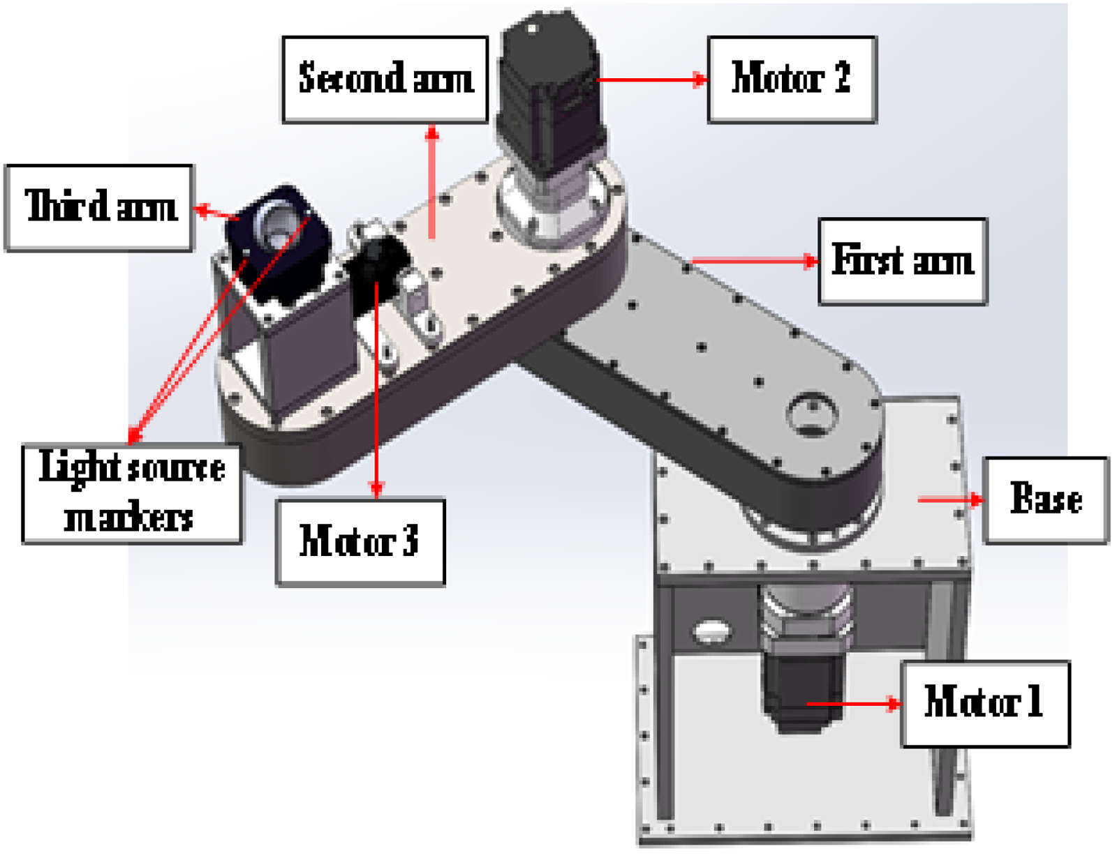
3D model drawing of the planar manipulator.

A schematic diagram of the plane manipulator is obtained with the base as the vertical projection plane, as shown in Figure 4.

Figure 4.

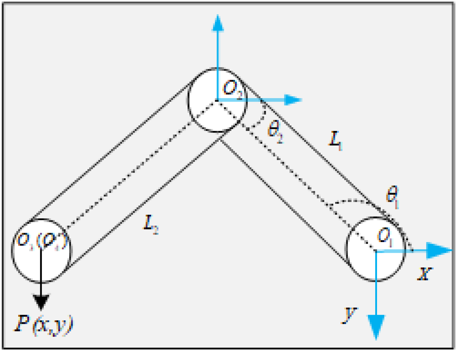
Schematic diagram of the manipulator vertical projection.

The theoretical length of the first arm, L₁ is the straight-line distance between O₁ and O₂, and θ₁ is the angle between the first arm and the X-axis in a clockwise direction. The theoretical length of the second arm L₂ is the straight-line distance between O₂ and O₃, and θ₂ is the angle between the second arm and the X-axis in a clockwise direction. The third arm L₃ is the straight-line distance between O₃ and O₄, because it is perpendicular to the end projection of the second arm and rotates coaxically with the end, O₃ coincides with the perpendicular projection of O₄, so the theoretical arm length L₃ of the third arm is 0 mm. P(x,y) is the end position of the manipulator. Establish the relationship between the ideal end position and the joint angle:

\begin{aligned} T & = A_{1} \cdot A_{2} \cdot A_{3} \\ = [\begin{matrix} \cos θ_{1} & - \sin θ_{1} & 0 & L_{1} \cos θ_{1} \\ \sin θ_{1} & \cos θ_{1} & 0 & L_{1} \sin θ_{1} \\ 0 & 0 & 1 & 0 \\ 0 & 0 & 0 & 1 \end{matrix}] \cdot [\begin{matrix} \cos θ_{2} & - \sin θ_{2} & 0 & L_{2} \cos θ_{2} \\ \sin θ_{2} & \cos θ_{2} & 0 & L_{2} \sin θ_{2} \\ 0 & 0 & 1 & d_{2} \\ 0 & 0 & 0 & 1 \end{matrix}] \cdot [\begin{matrix} \cos θ_{3} & - \sin θ_{3} & 0 & 0 \\ \sin θ_{3} & \cos θ_{3} & 0 & 0 \\ 0 & 0 & 1 & d_{3} \\ 0 & 0 & 0 & 1 \end{matrix}] \end{aligned}

(1)

T = [\begin{matrix} \cos (θ_{1} + θ_{2}) & - \sin (θ_{1} + θ_{2}) & 0 & L_{1} \cos (θ_{1}) + L_{2} \cos (θ_{2} + θ_{1}) \\ \sin (θ_{1} + θ_{2}) & \cos (θ_{1} + θ_{2}) & 0 & L_{1} \sin (θ_{1}) + L_{2} \sin (θ_{2} + θ_{1}) \\ 0 & 0 & 1 & d_{2} + d_{3} \\ 0 & 0 & 0 & 1 \end{matrix}]

(2)

[\begin{matrix} L_{1} \cos (θ_{1}) + L_{2} \cos (θ_{2} + θ_{1}) \\ L_{1} \sin (θ_{1}) + L_{2} \sin (θ_{2} + θ_{1}) \\ d_{2} + d_{3} \\ 1 \end{matrix}] = [\begin{matrix} x \\ y \\ z \\ 1 \end{matrix}]

(3)

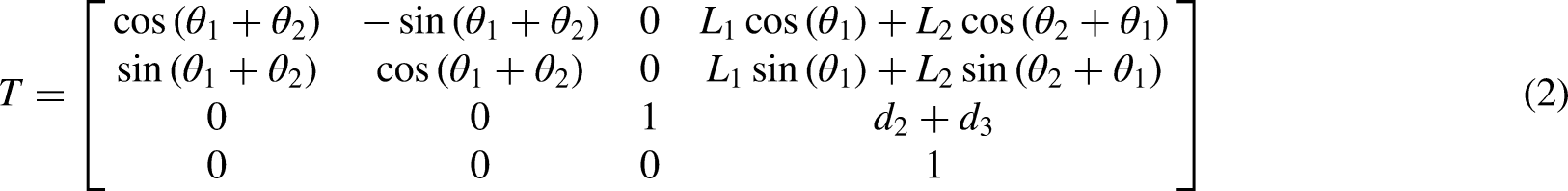
Among them, A₁, A₂, and A₃ in equation (1) are the transformation matrices of the three joint degrees of freedom of the manipulator, respectively. θ_i is the angle of rotation of the joint i, d_i is the offset distance between the axes of adjacent connecting rods, L_i is the length of the connecting rod i. According to the correspondence of equation (x), the forward kinematics model of the manipulator is expressed as follows:

{\begin{matrix} x = L_{1} \cos θ_{1} + L_{2} \cos (θ_{1} + θ_{2}) \\ \begin{matrix} y = L_{1} \sin θ_{1} + L_{2} \sin (θ_{1} + θ_{2}) \\ z = d_{2} + d_{3} \end{matrix} \end{matrix}

(4)

It is worth noting that the end of the manipulator involved in this paper moves in the XOY plane with the same z-axis height, and the Z-axis height is kept at d₂ + d₃, so the position change of the XOY plane is mainly considered in the absolute positioning study. According to the inverse solution of the formula, the relationship between angle and position is obtained as follows.

θ_{1} = 2_{atan} (\frac{\sqrt{- {(A^{2} + B^{2})}^{2} + 2 A^{2} (L_{1}^{2} + L_{2}^{2}) + 2 B^{2} (L_{1}^{2} + L_{2}^{2}) - {(L_{1}^{2} - L_{2}^{2})}^{2}} + 2 B L_{1}}{A^{2} + 2 A L_{1} + B^{2} + L_{1}^{2} - L_{2}^{2}})

(5)

θ_{2} = - 2_{atan} (\frac{\sqrt{- {(A^{2} + B^{2})}^{2} + 2 A^{2} (L_{1}^{2} + L_{2}^{2}) + 2 B^{2} (L_{1}^{2} + L_{2}^{2}) - {(L_{1}^{2} - L_{2}^{2})}^{2}} - 2 B L_{1}}{A^{2} + 2 A L_{1} + B^{2} - L_{1}^{2} + L_{2}^{2}}) + θ_{1}

(6)

Due to the limitation of part machining accuracy and manual assembly process, there is a systematic deviation between the actual kinematic model parameters of the plane manipulator (especially the actual length of the connecting rod) and the theoretical parameters, which leads to kinematic calibration errors). In addition, vision-based end-position measurement systems introduce systematic measurement errors that need to be compensated for by incorporating other high-precision measurement techniques. In this paper, the Leica AT960 laser tracker with a measurement accuracy of 0.01 mm is introduced as a calibration tool for the visual measurement system, and the visual measurement error of the measurement point is obtained by establishing the mapping relationship between the laser tracker data and the visual measurement error.

Monocular vision measurement error analysis for the planar manipulator

The process of monocular vision measurement

In the process of the experiments, the circular light source marks at the end of the manipulator are measured by the vision. The circular light source marks is shown as Figure 5.The pixel information of the end position of the manipulator is then transformed into the real spatial position of the end of the manipulator.

Figure 5.

Distribution of the markers and tracking balls.

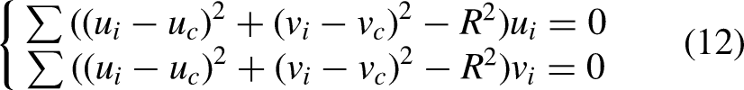
Due to the irregular edges of the circular marker pixels measured by the vision and the need to fit these pixels to a pixel center of gravity to represent the end position of the manipulator,¹⁴ the edge pixels of the circular marker are extracted, and then the center of the circle is fitted with the least square method as a series of discrete coordinate points.

For a set of discrete measurement points $(x_{i}, y_{i}) (i = 1, 2, \dots, m)$ , we let the center of the ideal circle be $P_{c} (x_{c}, y_{c})$ and the radius be R.¹⁵ Usually, the requirement for least-squares fitting is that the sum of squares of the distances reaches minimum, which can be depicted in the following expression:

f = \sum ((x_{i} - x_{c})^{2} + (y_{i} - y_{c})^{2} - R^{2})^{2}

(7)

The above equation can be further simplified as follows:

g (x, y) = (x - x_{c})^{2} + (y - y_{c})^{2} - R^{2}

(8)

The least-squares method should satisfy the following requirement:

\frac{\partial f}{\partial R} = 0

(9)

\sum g (x_{i}, y_{i}) = 0

(10)

Moreover, we make the following assumptions:

{\begin{matrix} u_{i} = x_{i} - \bar{x} \\ u_{c} = x_{c} - \bar{x} \\ v_{i} = y_{i} - \bar{y} \\ v_{c} = y_{c} - \bar{y} \end{matrix}

(11)

where

(u_{i}, v_{i})

is the offset of the data point

(x_{i}, y_{i})

relative to the center

({\bar{x}}_{i}, {\bar{y}}_{i})

of all data points;

(u_{c}, v_{c})

is the coordinate of the data point

(x_{c}, y_{c})

in the coordinate system (with data center

({\bar{x}}_{i}, {\bar{y}}_{i})

as the origin) after translation. Substituting equation (11) into equations (9)-(10), on can obtain the following:

{\begin{matrix} \sum ({(u_{i} - u_{c})}^{2} + (v_{i} - v_{c})^{2} - R^{2}) u_{i} = 0 \\ \sum ({(u_{i} - u_{c})}^{2} + (v_{i} - v_{c})^{2} - R^{2}) v_{i} = 0 \end{matrix}

(12)

Rearranging this equation yields the following:

{\begin{matrix} u_{c} = \frac{\sum u_{i} v_{i} (\sum u_{i}^{2} v_{i} + \sum v_{i}^{3}) - \sum v_{i}^{2} (\sum u_{i}^{3} + \sum u_{i} v_{i}^{2})}{2 \sum u_{i} v_{i} (\sum u_{i} v_{i} - \sum u_{i}^{2})} \\ v_{c} = \frac{\sum u_{i} v_{i} (\sum u_{i} v_{i}^{2} + \sum u_{i}^{3}) - \sum u_{i}^{2} (\sum v_{i}^{3} + \sum u_{i}^{2} v_{i})}{2 \sum u_{i} v_{i} (\sum u_{i} v_{i} - \sum u_{i}^{2})} \end{matrix}

(13)

{\begin{matrix} x_{c} = u_{c} - \bar{x} \\ y_{c} = v_{c} - \bar{y} \end{matrix}

(14)

R = \sqrt{\frac{\sum ({(x_{i} - x_{c})}^{2} + (y_{i} - y_{c})^{2})}{N}}

(15)

The image containing the feature marker information was fitted to the center of the circle by the least-squares method, as shown in Figure 6.

Figure 6.

Edge fitting diagram of two circular markers. (a) Edge fitting diagram of the first marker. (b) Edge fitting diagram of the second marker.

The measurement error analysis of monocular vision

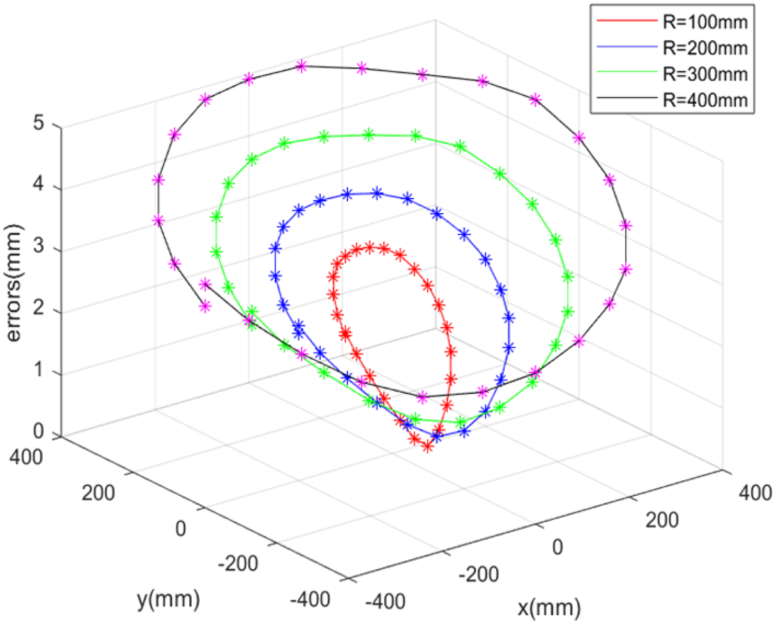
In this experiment, visual measurement is designed for all kind of different trajectories, such as circular trajectories. When the planar manipulator moves from one point to another point, a certain positioning error will occur compared with the ideal trajectory. The vision measures 25 discrete points on the circular trajectory with radii of 100 mm, 200 mm, 300 mm, and 400 mm, respectively. The difference between the measured data and the theoretical data is calculated to obtain the positioning and measurement errors.

The visual measured data includes the actual manipulator movement data and the visual measured errors, as shown in the following equation.

M_{v} = M_{p} + E_{v} = (M_{d} + E_{p}) + E_{v}

(16)

where M_v is the visual measurement data, M_p is the actual motion data of the manipulator, E_v is the visual measurement errors, M_d is the expected motion data of the manipulator, and E_p is the manipulator motion errors.

The laser tracker measured data includes the actual manipulator movement data and the measured errors of laser tracker, as shown in the following equation.

M_{l} = M_{p} + E_{l} = (M_{d} + E_{p}) + E_{l}

(17)

where M_l is the visual measurement data, M_p is the actual motion data of the manipulator, E_l is the errors of the laser tracker, M_d is the expected motion data of the manipulator, and E_p is the manipulator motion errors.

The distributed points measured in the end of the manipulator are shown in Figure 7.

Figure 7.

Distribution of measurement points in the end of the manipulator.

As shown in Figures 8 and 9, when monocular vision is employed to measure the trajectory of planar manipulator, it can be noted that the larger the working range of the manipulator's motion will lead to the greater the values of $(E_{p} + E_{v})$ and $(E_{p} + E_{l})$ . Additionally, if the positions are farther from the optical center, the field of view distortion errors will become more pronounced. Even after image distortion processing, the vision may still exhibit systematic errors. Consequently, as the motion range of the manipulator expands, the visual measurement errors also tend to increase. The laser tracker is also used to measure 25 discrete points on the circular trajectory with radii of 100 mm, 200 mm, 300 mm, and 400 mm.

Figure 8.

Manipulator motion errors and visual measured errors $(E_{p} + E_{v})$ .

Figure 9.

Manipulator motion errors and laser measured errors $(E_{p} + E_{l})$ .

The high-precision measurement of the laser tracker is used to compare the measurement accuracy of the vision and compensate the measurement errors of the vision. The results of visual measurement and laser tracker measurement are compared in Figure 10.

Figure 10.

Visual measured errors relative to laser tracker $(E_{v} - E_{l})$ .

Three experiments of the different trajectories are conducted to compare the errors for the laser tracking and the visual measurement. Then, the correlation analysis of the experiments is used to observe the correlation significance of the visual measurement errors.

Figure 11 and Table 1 show the results of the correlation analysis of circular trajectories with radii between 100 mm and 400 mm. The correlations of the four circular trajectories were 0.991, 0.996, 0.993 and 0.995, respectively. It can be seen that the correlation of visual measurement errors is very significant, and the correlation is greater than 0.95, indicating that the detection data obtained by the visual measurement system after many experiments are stable and the experimental data fluctuates little. There is a high correlation and high regularity of visual measurement errors in the whole motion space, which provides reliable theoretical support for the subsequent establishment of visual measurement error mapping relationship and improvement of the measurement accuracy of visual measurement system.

Figure 11.

Correlation of visual measurement errors.

Table 1.

Correlation analysis of the different trajectories.

Measurement trajectories	Coefficient of correlation
Radius of 100 mm	0.991
Radius of 200 mm	0.996
Radius of 300 mm	0.993
Radius of 400 mm	0.995

The vision measurement error prediction across the visual field range

After obtaining the visual measurement error data in The measurement error analysis of monocular vision section, this study employs the linear IDW method and nonlinear RBF neural network to interpolate the error data from discrete points, which can predict the visual measurement errors for the entire measurement field.

In this paper, a simple IDW linear fitting method is chosen because of its fast computational speed. However, it has limited predictive accuracy. In order to further improve the prediction accuracy of visual measurement error, the RBF neural network was selected. The reasons for choosing RBF neural network for prediction are: firstly, the RBF network can more accurately approximate the laws of the data, which is suitable for dealing with complex relationships in the data. Second, the training process of RBF neural networks is relatively simple, and the prediction speed of RBF networks is relatively fast compared to some other neural network architectures. This feature significantly reduces the time required for data processing in feedback-controlled experiments.

The effectiveness of both methods is compared, which are applied to improve the accuracy of the visual measurement and minimize the absolute positioning error of the planar manipulator. The angles of each joints are adjusted according the absolute positioning error and achieve the high-precision visual servo control for the planar manipulator via feedback control.

Inverse distance weighting spatial interpolation-based prediction method

In order to obtain the measurement errors across the whole visual field of the plane manipulator, the laser tracker is introduced to compare with the visual measurement. The result is used as the compensation to improve the measurement accuracy of vision. Here, the IDW spatial interpolation method is used to predict the visual measurement errors of the whole movement space.

As a linear interpolation method, IDW is one of the most commonly used spatial interpolation methods, where the sample points closer to the interpolation points are given a greater weight.^16,17 Moreover, their weight contribution is inversely proportional to the distance, and it can be calculated by the following equations.

Z (x, y) = \frac{\sum_{i = 1}^{n} \frac{Z_{i}}{d_{i}}}{\sum_{i = 1}^{n} \frac{1}{d_{i}}}

(18)

Z_{i} = \sqrt{x_{i}^{2} + y_{i}^{2}}

(19)

d_{i} = \sqrt{{(x - x_{i})}^{2} + {(y - y_{i})}^{2}}

(20)

where

Z (x, y)

is the value of the point to be estimated,

(x, y)

is the location of the point to be estimated,

Z_{i}

is the number of known points, and

d_{i}

is the distance between the estimated point and the known point.

Some regular spatial points are selected by the laser tracker to obtain the visual measurement errors. These points are used as training data, and other undetectable position points are selected as test data. The IDW method can predict the visual measurement errors of these undetectable locations, then one can obtain the prediction accuracy by comparing them with the real measured data via laser tracker (Figure 12).

Figure 12.

IDW spatial interpolation of estimated location points. IDW: inverse distance weighting.

It can be seen that the trend of visual measurement error of predicted points of Figure 13(b) is very close to that of visual measurement errors of Figure 13(a), which indicates that the visual measurement error of unknown points can be roughly obtained from known points using the IDW spatial interpolation method. In order to verify the specific prediction effect of the IDW spatial interpolation method, the prediction results of the predicted points were compared with the actual measurement results as shown in Figure 14.

Figure 13.

Surface diagram of the known points errors and prediction points errors. (a) Surface plot of known points visual measurement errors. (b) Surface plot of prediction points visual measurement errors.

Figure 14.

Actual measurement errors and the IDW prediction errors. IDW: inverse distance weighting.

As shown in Table 2, the mean errors of different circle trajectories are compared for actual visual measurements and IDW predictions. The estimated accuracy of the linear IDW method for random position visual measurement errors is 65.7% for circular tracks with radius 150 mm, 79.6% for circular tracks with radius 250 mm, and 85.3% for circular tracks with radius 350 mm, respectively. The prediction accuracy of linear IDW method is fluctuating for the circle trajectories with different radii. It indicates that the non-linearity in the visual measurement system has important impact on the prediction accuracy, which limits the effects of the linear IDW spatial interpolation method.

Table 2.

The IDW predicted the accuracy of the visual measurement errors.

Visual measurement errors under different circle trajectories	Actual mean error for each trajectory	IDW prediction mean errors	Prediction accuracy
Circle with radius 150mm	0.561mm	0.368 mm	65.7%
Circle with radius 250mm	1.020 mm	0.812 mm	79.6%
Circle with radius 350mm	1.621 mm	1.383mm	85.3%

IDW: inverse distance weighting.

Prediction method based on radial basis neural network

IDW spatial interpolation is a kind of weight coefficient assigned based on the distance between the estimated positions and the known positions. The data information of the estimated positions is obtained according to the weight relationship. However, the nonlinear motion data cannot be well estimated by IDW spatial interpolation, which can be solved by the RBF neural network spatial interpolation. Using the RBF as the activation function, RBF neural network can deal with the regularity that is difficult to parse in the system. It has good generalization ability and a fast-learning convergence speed.

The RBF neural network is a forward network composed of the input layer, the hidden layer, and the output layer.¹⁸ The first layer is the input layer, which is composed of input data. The second layer is the hidden layer, which is the transformation function of each element. The low-dimensional input is mapped to a high-dimensional space by a nonlinear Gaussian function. The third layer is the output layer, which responds to the input signals. 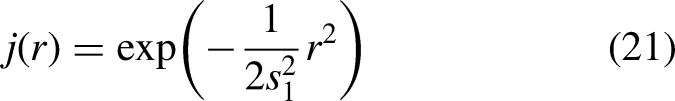The hidden layer to the output layer can be used to calculate the output value in the output layer by linear weighting, where the weight is w_i.¹⁹ In this study, the activation function used in the RBF neural network is the Gauss RBF.²⁰

j (r) = \exp (- \frac{1}{2 s_{1}^{2}} r^{2})

(21)

Y_{i} = \sum_{i = 1}^{n} w_{i} \exp (- \frac{1}{2 s_{1}^{2}} | | x_{j} - x_{i} | |^{2})

(22)

where

| | x_{j} - x_{i} | |

denotes the norm, x_j is the j_th input data, x_i is the data center point of sample i,

s_{1}

is the width parameter of the function, which controls the radial range of the function. w_i is the synaptic weight between the j_th node of the hidden layer and the K_th node of the output layer.

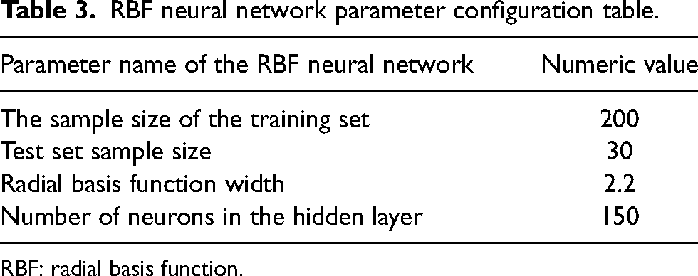
In this paper, 200 positions were collected as the training set sample and 30 positions were collected as the test set sample, and each sample was composed of three data elements: position x, position y, and the visual measurement error of the position. Taking position x and position y as inputs, and taking the visual measurement error of the position as output, the mapping relationship of the RBF neural network was established. The minimum root mean square error value was obtained by manually adjusting the width of the RBF, and then the optimal RBF neural network model was determined. Table 3 lists the parameters of the RBF neural network configured in this document.

Table 3.

RBF neural network parameter configuration table.

Parameter name of the RBF neural network	Numeric value
The sample size of the training set	200
Test set sample size	30
Radial basis function width	2.2
Number of neurons in the hidden layer	150

RBF: radial basis function.

In the experiment, in order to test the prediction effect of RBF neural network mapping relationship and the repeatability of the prediction results, in this paper, the visual measurement error data of 24 points on discrete circles with radii of 150 mm, 250 mm, and 350 mm were collected as the input data of RBF neural network, and the results of three predictions were made and the output visual measurement error results were recorded as shown in Table 4. Finally, the prediction accuracy is obtained by comparing the output results with the actual measured visual measurement error data at this point, and the prediction accuracy is shown in Table 5.

Table 4.

Standard deviation of prediction at 72 points.

Visual measurement errors under different circle trajectories	First RBF prediction output	Second RBF prediction output	Third RBF prediction output	Standard deviation
Circle with radius 150mm	0.504 mm	0.510 mm	0.510 mm	0.0035 mm
Circle with radius 250mm	0.891 mm	0.896 mm	0.898 mm	0.0036 mm
Circle with radius 350mm	1.545 mm	1.541 mm	1.549 mm	0.0040 mm

RBF: radial basis function.

Table 5.

Prediction accuracy of the RBF neural network.

Visual measurement errors under different circle trajectories	Actual mean errors for each trajectory	Predicted mean errors by RBF	Prediction accuracy
Circle with radius 150mm	0.561 mm	0.508 mm	90.5%
Circle with radius 250mm	1.020 mm	0.894 mm	87.6%
Circle with radius 350mm	1.621 mm	1.545 mm	95.3%

RBF: radial basis function.

From Table 4, it can be seen that the standard deviation of the visual measurement errors predicted by the RBF neural network for points on different discrete circles is less than 0.004 mm. This indicates a high absolute repeatability of its predictions and a very small range of measurement result fluctuations.

As shown in Table 5, the mean errors of different circle trajectories are compared for actual visual measurements and RBF neural network predictions. The estimated accuracy of the RBF neural network method for random position visual measurement errors is 90.5% for circular tracks with radius 150 mm, 87.6% for circular tracks with radius 250 mm, and 95.3% for circular tracks with radius 350 mm, respectively. The prediction accuracy of RBF neural network is greatly enhanced for the circle trajectories with different radii. It indicates that RBF neural network can deal with the non-linearity in the visual measurement system.

It can be seen that the trend of estimated errors of Figure 15(b) is very close to that of undetectable errors of Figure 15(a), which indicates that RBF neural network can well predict the estimated errors of the unknown points. In order to verify the specific prediction effect of the RBF neural network, the prediction results of the predicted points were compared with the actual measurement results as shown in Figure 16.

Figure 15.

Surface diagram of the raw data errors and interpolation errors. (a) Surface diagram of the raw data errors. (b) Surface diagram of the interpolation errors.

Figure 16.

Actual measurement errors and the RBF neural network prediction errors. RBF: radial basis function.

As can be seen from Table 6, the prediction accuracy of the RBF neural network is far better than that of IDW method. Then, the experiments of the absolute positioning for the planar manipulator use the RBF neural network method to predict the visual measurement errors. The RBF neural network method-based high-precision vision can replace the laser tracker to collect the positioning error and complete the feedback control for the planar manipulator.

Table 6.

The comparisons for the IDW and RBF method.

Visual measurement errors under different circle trajectories	Prediction accuracy of IDW	Prediction accuracy of RBF
Circle with radius 150mm	65.7%	90.5%
Circle with radius 250mm	79.6%	87.6%
Circle with radius 350mm	85.3%	95.3%
Overall mean	76.9%	91.1%

RBF: radial basis function; IDW: inverse distance weighting.

Visual measurement error prediction-based feedback control

As shown in The vision measurement error prediction across the visual field range section, the RBF neural network-based method has good performance to predict the visual measurement errors, which can be used to calculate the position deviations. According to the kinematic inverse solution of the planar manipulator, the compensations of joint's angles for feedback control are also computed for feedback control is to improve the movement accuracy of the planar manipulator. The control process can be simplified to vision and the laser tracker measures the end position at the same time to obtain the data of visual measurement errors. To collect the multiple spatial location data and train the RBF neural network, the visual measurement distribution can be predicted and used to compensate for the visual measurement data. This process will obviously enhance the positioning accuracy for the motion of the planar manipulator.

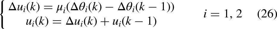
According to the experimental flow chart shown in Figure 17, firstly, the visual measurement system obtains the end position of the manipulator (x_c, y_c) from the acquired images, and the data contains the visual measurement error in addition to the actual end-position information of the manipulator. (x_c, y_c) is used as the input of the RBF neural network model, and the visual measurement error Ec of the position is output, then the visual measurement position (x_c, y_c)-E_c obtains the actual end position of the manipulator (x_a, y_a), and then the difference between the actual end position and the theoretical position (x_d, y_d) is used to obtain the absolute positioning error (Δx, Δy) = (x_d, y_d)−(x_a, y_a). Then, the inverse solution of the kinematic equation is used to calculate the joint angle compensation (Δθ₁, Δθ₂) required for the absolute positioning error. These compensation quantities (Δθ₁, Δθ₂) are multiplied by the proportional control parameters (k₁, k₂) to obtain the feedback control inputs (u₁, u₂), where these proportional control parameters are the angle and pulse conversion parameters, which are the factory setting parameters of the motor. The mathematical models for the feedback control are involved as follows.

{\begin{matrix} Δ x = x_{a} - x_{o} \\ Δ y = y_{a} - y_{o} \end{matrix}

(23)

Δ θ_{1} = 2 \arctan (\frac{\sqrt{- {(Δ x^{2} + Δ y^{2})}^{2} + (2 Δ x^{2} + 2 Δ y^{2}) (L_{1}^{2} + L_{2}^{2}) - {(L_{1}^{2} - L_{2}^{2})}^{2}} + 2 Δ y L_{1}}{Δ x^{2} + 2 Δ x L_{1} + Δ y^{2} + L_{1}^{2} - L_{2}^{2}})

(24)

Δ θ_{2} = Δ θ_{1} - 2 \arctan (\frac{\sqrt{- {(Δ x^{2} + Δ y^{2})}^{2} + (2 Δ x^{2} + 2 Δ y^{2}) (L_{1}^{2} + L_{2}^{2}) - {(L_{1}^{2} - L_{2}^{2})}^{2}} - 2 Δ y L_{1}}{Δ x^{2} + 2 Δ x L_{1} + Δ y^{2} - L_{1}^{2} + L_{2}^{2}})

(25)

{\begin{matrix} Δ u_{i} (k) = μ_{i} (Δ θ_{i} (k) - Δ θ_{i} (k - 1)) \\ u_{i} (k) = Δ u_{i} (k) + u_{i} (k - 1) \end{matrix} \begin{matrix} i = 1, 2 \end{matrix}

(26)

where

u_{1}

is the input of the unit angle conversion pulse of the motor 1 and

u_{2}

is the input of the unit angle conversion pulse of the motor 2,

μ_{i} = [\begin{matrix} k_{1} & k_{2} \end{matrix}]

are angle and pulse conversion parameters of the two motors (k₁ = 500 and k₂ = 450).

Figure 17.

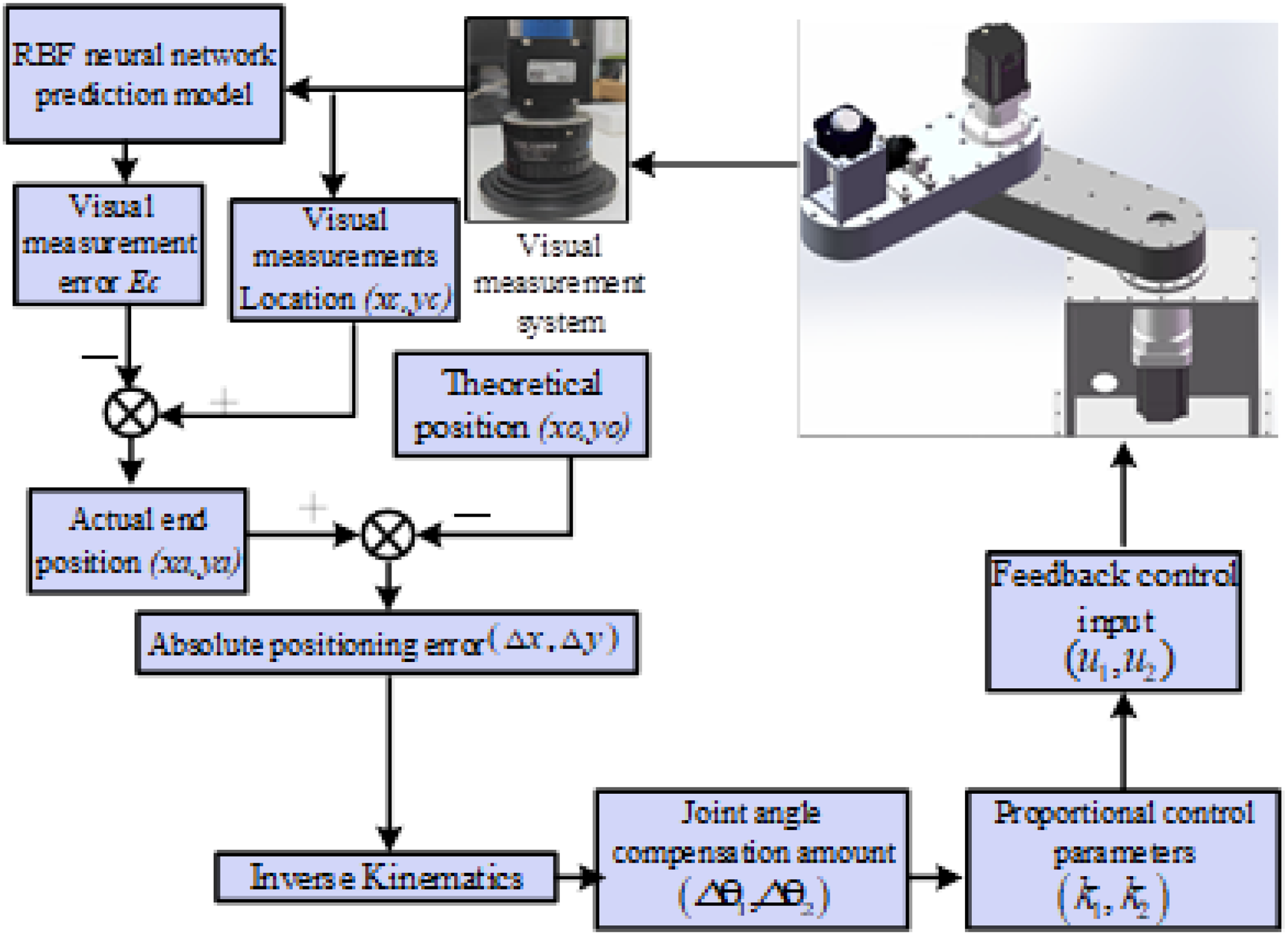
Absolute positioning error feedback control flow chart.

In order to verify the effect of improving the absolute positioning accuracy of the planar manipulator by combining the position error of the visual measurement end with the above-mentioned feedback control method after the RBF neural network improves the visual measurement accuracy. In this section, four rings with a radius of 200 mm and a center position of (−200 mm, −200 mm), (−200 mm, 200 mm), (200 mm, 200 mm), and (200 mm, −200 mm) are selected, and 25 points are selected from each ring at equal distances as the desired points. The distribution of these 100 points is shown in Figure 18.

Figure 18.

Position points of the discrete trajectories for experiments.

As shown in Table 7 and Figure 19, with the help of the RBF neural network for the measurement error predictions, the mean positioning deviations of the end of the planar manipulator are all reduced significantly. The mean deviation of the circular trajectory with the center position of (−200 mm, −200 mm) is 0.185 mm, which indicates that the absolute positioning accuracy for the feedback control is improved by 87.7%, and that with the center position of (−200 mm, 200 mm) is 0.174 mm, which indicates that the absolute positioning accuracy for the feedback control is improved by 87.2%. Similarly, the mean deviation of the circular trajectory with the center position of (200 mm, 200 mm) is 0.180 mm, which indicates that the absolute positioning accuracy for the feedback control is improved by 85.7%, while that with the center position of (200 mm, −200 mm) is 0.176 mm, which indicates that the absolute positioning accuracy for the feedback control is improved by 85.1%. As a whole, the average improved accuracy is 86.4% after the feedback control for the planar manipulator.

Figure 19.

The performance of the feedback control for the four circle trajectories.

Table 7.

The feedback control of absolute positioning errors.

Feedback controltrajectories	Mean error before feedback control	Mean error values after feedback control	Improve control accuracy
Center of a circle: (−200 mm, −200 mm)	1.514 mm	0.185 mm	87.7%
Center of a circle: (−200 mm, 200 mm)	1.358 mm	0.174 mm	87.2%
Center of a circle: (200 mm, 200 mm)	1.260 mm	0.180 mm	85.7%
Center of a circle: (200 mm, −200 mm)	1.138 mm	0.170 mm	85.1%

Conclusions

In this paper, a monocular visual measurement error prediction and feedback control method was proposed for a planar manipulator. Firstly, the monocular vision was used to capture the markers and extract pixel information regarding the manipulator's endpoint, while the data from the laser tracker was converted into the same coordinate system to compare and compensate the visual measurement errors. Because the RBF neural network can obtain a higher accuracy of visual measurement than the IDW spatial interpolation, then, the continuous errors of the entire workspace were obtained using visual measurement error prediction based on RBF neural network spatial interpolation. Finally, the visual measurement error prediction-based feedback controls were conducted for the positioning of planar manipulator. The experiments show that the feedback control of the planar manipulator by visual measurement improves the absolute positioning accuracy of the planar manipulator to 86.4%. The mean absolute positioning errors of the four eccentric circles are reduced from 1.318 mm to 0.178 mm.

Therefore, by fusing the improved accuracy of the visual measurement system and the feedback control of the end-position error of the plane manipulator, the real-time interaction of the end-position data and the absolute positioning accuracy are greatly improved. Experiments show that the absolute positioning accuracy of the manipulator can be significantly improved by using the visual measurement system after improving the measurement accuracy and the inverse kinematic feedback control method, and the absolute positioning accuracy can be kept within the range of 0.2mm. At present, the absolute positioning accuracy of industrial robots from various large robot brands, such as KUKA and ABB, is also around 0.2 mm. Based on this, the low-cost monocular camera is used as the online measurement device, and the RBF neural network is used as the visual measurement error compensation algorithm to improve the measurement accuracy of the vision system, so as to replace the high-cost, offline measurement laser tracker.

Footnotes

Acknowledgment

The work presented in this paper was funded by Guangdong Basic and Applied Basic Research Foundation (2022A1515140156) and Guang dong Universities new information field (2021ZDZX1057).

Author contributions

YC and MJ conceived and designed the study. JZ and LX conducted data gathering. ZX performed statistical analyses. JZ and MJ wrote the article.

Declaration of conflicting interests

The authors declared no potential conflicts of interest with respect to the research, authorship, and/or publication of this article.

Ethical approval

Not applicable.

Funding

The authors disclosed receipt of the following financial support for the research, authorship, and/or publication of this article: This work was supported by the Mian Jiang, (grant number 2021ZDZX1057, 2022A1515140156).

ORCID iD

Jiahua Zou

Data availability statement

Data sharing not applicable to this article as no datasets were generated or analyzed during the current study.

References

Wei

Wenhe

Wei

. Theory and experiment of industrial robot accuracy compensation method based on spatial interpolation. J Mech Eng 2013; 49: 42–48.

Zhu

Yin

. Research Status of Robot Calibration Technology. In: 2018 5th International Conference on Information, Cybernetics, and Computational Social Systems (ICCSS), Hangzhou, China, 2018, pp.424–428.

Shirafuji

Goto

Zhang

, et al. Visual-biased observability index for camera-based robot calibration. J Mech Robot 2024; 16: 051010.

Chen

Yang

. High Precision Pose Measurement for Humanoid Robot Based on PnP and OI Algorithms[C], Chinese Academy of Sciences, Beijing 100190, P. R. China, 2010.

Briot

Kaci

Boudaud

, et al. Design of an accurate and stiff wooden industrial robot: first steps toward robot eco-sustainable mechanical design. J Mech Robot 2020; 12: 051015.

Jiawei

Tiansheng

Ruijie

. Design of industrial robot grasping system based on monocular vision. J Yancheng Institute Technol (Natural Science Edition) 2023; 36: 33–37.

Wang

Ping

. Research on the kinematic parameter identification of manipulator based on the assistant location by stereo vision. Chinese J Eng Design 2018; 25: 27–34.

Chen

Zhang

. A calibration method for enhancing robot accuracy through integration of kinematic model and spatial interpolation algorithm. J Mech Robot 2021; 13: 061013.

Yanqiong

Kefan

Rongsheng

, et al. Kinematic parameter identification of industrial robot based on binocular vision. Laser & Optoelectronics Progress 2023; 60: 272–280.

10.

Davila-Rios

Lopez-Juarez

Mendez

, et al. A fuzzy approach for on-line error compensation during robotic welding. In: 2016 6th International Conference on Computers Communications and Control (ICCCC), Warsaw: IEEE, 2016: 264–270.

11.

Wenjing

Zihang

Jianguo

, et al. Workpiece recognition and positioning using industrial robotic arm assisted machine vision. Mod Mach Tool Autom Manuf Tech 2024; 01: 53–57, 62.

12.

Junnan

Shuang

. 2-DOF manipulator control system based on visual location. Machinery & Electronics 2008; 02: 49–52.

13.

Jiawei

Yuqing

Xiaopeng

, et al. Design of manipulator target positioning system based on monocular vision. Opticai. Technique 2019; 45: 6–11.

14.

Chernov

Lesort

. Least squares fitting of circles. J Math Imaging Vis 2005; 23: 239–252.

15.

Liu

Zhang

Gui

, et al. Fitting plane circular curve with constrained least squares method. J Computer-Aided Design Graphics 2004; 10: 1382–1385.

16.

Wong

. An adaptive inverse-distance weighting spatial interpolation technique. Comput Geosci 2008; 34: 1044–1055.

17.

Chen

Liu

. Estimation of the spatial rainfall distribution using inverse distance weighting (IDW) in the middle of Taiwan. Paddy Water Environ 2012; 10: 209–222.

18.

Yingwei

Sundararajan

Saratchandran

. Performance evaluation of a sequential minimal radial basis function (RBF) neural network learning algorithm. IEEE Trans Neural Netw 1998; 9: 308–318.

19.

Sharkawy

. Principle of neural network and its main types. J Adv Appl Comput Mathematics 2020; 7: 8–19.

20.

Tran

Kang

. A novel adaptive finite-time tracking control for robotic manipulators using nonsingular terminal sliding mode and RBF neural networks. Int J Prec Eng Manuf 2016; 17: 863–870.

Monocular vision measurement error prediction and feedback control for a planar manipulator

Abstract

Keywords

Introduction

The kinematics model of the planar manipulator

The planar manipulator

The kinematics model of the planar manipulator

Monocular vision measurement error analysis for the planar manipulator

The process of monocular vision measurement

The measurement error analysis of monocular vision

The vision measurement error prediction across the visual field range

Inverse distance weighting spatial interpolation-based prediction method

Prediction method based on radial basis neural network

Visual measurement error prediction-based feedback control

Conclusions

Footnotes

Acknowledgment

Author contributions

Declaration of conflicting interests

Ethical approval

Funding

ORCID iD

Data availability statement

References