Sage Journals: Discover world-class research

Abstract

This paper proposes a variable impedance control strategy based on the singular perturbation method to address the challenges of achieving accurate impedance characteristics and mitigating stability degradation in two-degree-of-freedom planar SEA-driven robots. By decomposing the system into fast and slow subsystems, we control them separately to improve tracking performance, disturbance rejection, and impedance control. A MATLAB/Simulink model was developed for simulation and compared with a traditional PD controller. The results show that the proposed controller outperforms the PD controller, maintaining position errors under 10% and impedance errors under 30% of those seen with the PD controller under external force input. Additionally, experimental validation confirmed the controller's ability to optimally adjust robot stiffness in response to changes in the user's limb-end stiffness, supporting the assist-as-needed strategy.

Keywords

Adaptive impedance control singular perturbation theory SEA upper limb robot rehabilitation robot

Introduction

Patients with upper limb dysfunction often face barriers to adequate rehabilitation due to economic, resource, and time constraints. Leveraging neural plasticity,¹ rehabilitation robots aid in recovery by facilitating damage repair. Consequently, their integration into medical programs is increasingly seen as a practical and effective solution. Additionally, variable impedance control enhances rehabilitation by enabling adaptive force regulation, ensuring safer interactions, and improving therapeutic outcomes through individualized assistance tailored to patient needs.

In rehabilitation, common robot types include exoskeletons, exosuits, and end-effectors.^2–4 Exoskeletons offer multi-degree-of-freedom training but may cause discomfort due to mismatched joint axes.^5–7 Exosuits, based on human anatomy, may limit natural movement.⁸ End-effector robots ensure accurate positioning and comfort but lack flexibility, compromising safety and comfort in human-robot interactions.⁹ To overcome this, flexible elements like Series Elastic Actuators (SEA) and Variable Stiffness Actuators (VSA) have been introduced in end-effector robots, offering improved flexibility and user comfort. As a result, planar multi-degree-of-freedom SEA robots are now a leading design for rehabilitation.¹⁰

Control strategies for flexible robots are more complex than for rigid robots, particularly in multi-degree-of-freedom motion control for upper limb rehabilitation. These strategies must accommodate various training modes, such as assisted, power-assisted, and resistance training.^11,12 Current strategies include balance-based, challenge-based, adaptive, and tactile stimulation-based control. Electromyography (EMG)-based control is commonly used but challenging due to signal variability.¹³ For force and position control, impedance-based strategies are preferred,¹³ as they account for dynamic interactions and safety, making them more suitable for rehabilitation robotics.¹⁴ Impedance-based control is widely used in human-robot interactions to regulate force and position, ensuring the safety of rehabilitation robots.¹⁵ During therapy, the robot controls the patient's arm to follow a specific path, intervening when deviations occur. Ott et al. developed a passive control framework for flexible joint rehabilitation robots, incorporating internal torque feedback for impedance control, which was validated on DLR lightweight robots.¹⁶ However, this method is limited by fixed impedance parameters. Li et al. proposed an iterative learning impedance controller for SEA-driven robots, supporting dynamic stability.¹⁷ Sharifi et al. introduced a nonlinear adaptive bilateral impedance controller for tele-rehabilitation with multi-degree-of-freedom systems.¹⁸ Brahmi et al. developed an adaptive impedance control method for exoskeletons using a nonlinear time-delay disturbance observer.¹⁵ Current adaptive impedance control algorithms estimate real-time environmental dynamics and adjust robot impedance parameters accordingly.^19,20

Adaptive adjustment of impedance parameters and external disturbances increase the prominence of joint flexibility.²¹ SEA actuators, connected to flexible structures, complicate direct control, leading to challenges such as increased degrees of freedom, underactuation, vibration, and excessive contact forces from minor positional deviations. Consequently, adaptive impedance control must ensure system stability while modifying impedance parameters. Kronander et al. proposed constraints on variable impedance profiles for stability,²² while Liang et al. applied state-independent stability conditions for time-varying profiles.²³ Gosselin et al. examined the stability of macro-mini robot systems in human-robot interactions.²⁴ Thus, further research is needed on the stability of variable impedance control. Giovacchini et al. designed an APO control system with hierarchical torque and adaptive assistance levels. Given the coupled nature of flexible joint-driven systems, singular perturbation theory is applicable. This paper proposes a singular perturbation method using a variable impedance controller for a SEA-driven flexible upper limb rehabilitation robot, simplifying the system's model and enhancing controller stability.

This paper focuses on three main areas: (1) establishing the kinematic and dynamic models of a planar 2-DOF flexible robot; (2) designing a variable impedance controller based on impedance control theory and the singular perturbation method, with MATLAB/Simulink used for model construction and stability analysis; and (3) validating the controller's performance through simulation experiments, comparing it with a traditional PD controller. This comparison highlights the variable impedance controller's superior adaptability, stiffness control, and effectiveness in multivariable systems. An experimental platform further demonstrated the robot's ability to adjust its end-point stiffness using the assist-as-needed strategy, confirming the controller's effectiveness. The study emphasizes the variable impedance control of the SEA-driven 2-DOF planar robot with the singular perturbation method.

Flexible two-degree of freedom robot system

Kinematics model

The training diagram of the upper limb rehabilitation robot, which is based on the two-degree-of-freedom SEA-driven flexible joint, can be simplified as depicted in Figure 1(a). The forward kinematics formula for the two-degree-of-freedom upper limb rehabilitation robot is derived by considering point O as the reference center and it can be expressed as follows:

x_{p} = l_{1} \cos q_{1} + l_{2} \cos (q_{1} + q_{2})

(1)

y_{p} = l_{1} \sin q_{1} + l_{2} \sin (q_{1} + q_{2})

(2)

Figure 1

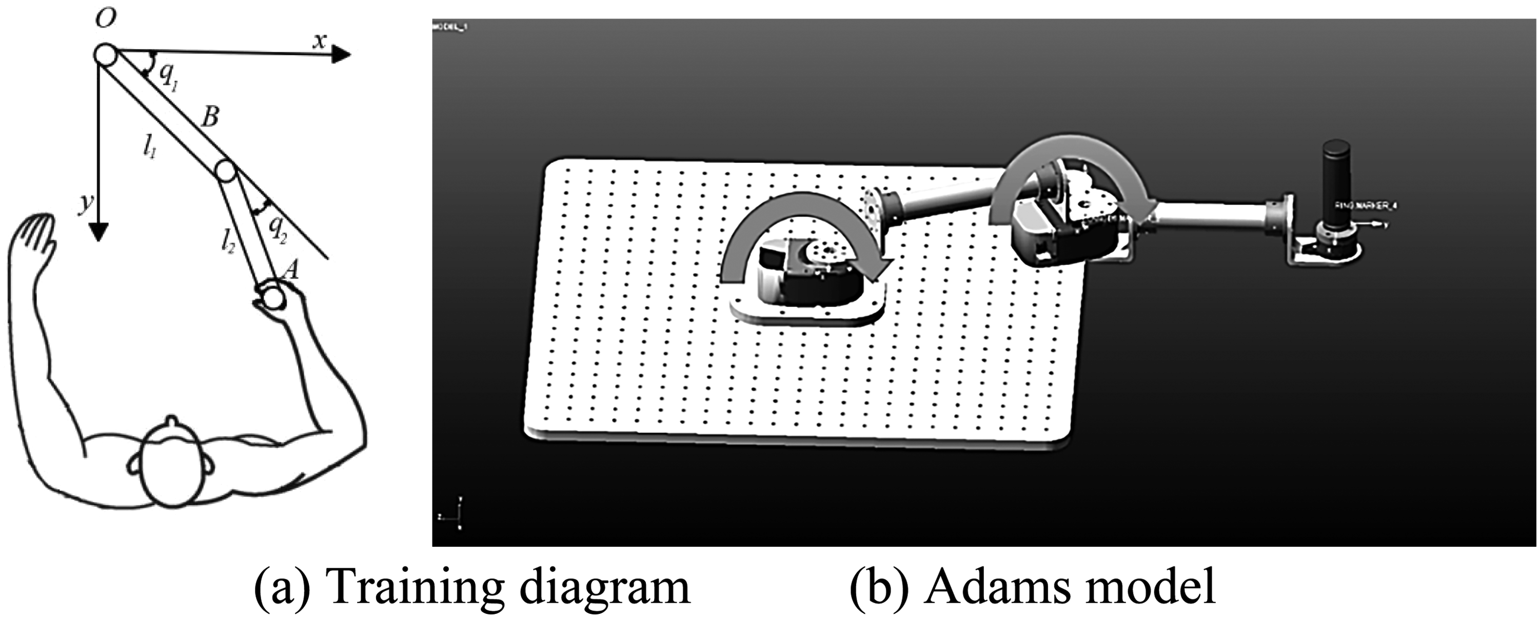
Flexible two-degree of freedom robot. (a) Training diagram (b) Adams model.

The variables $x_{p}$ and $y_{p}$ represent the abscissa and ordinate coordinates in Cartesian space.

The inverse kinematics formula can be derived from the direct kinematics as follows:

q_{1} = a \tan 2 (l_{1} y_{p} + l_{2} s_{2} x_{p}, l_{1} x_{p} + l_{2} c_{2} x_{p} + l_{2} s_{2} y_{p})

(3)

q_{2} = acos (\frac{x_{p}^{2} + y_{p}^{2} + l_{1}^{2} + l_{2}^{2}}{2 l_{1} l_{2}})

(4)

Figure 1(b) shows the Adams model of the SEA-driven flexible upper limb rehabilitation robot, initially designed in Creo and imported into Adams. Two joint connections were added, with the others fixed. A torsional spring (stiffness: 170 Nm/rad) simulates the elastomer at the motor and load ends, enabling kinematic simulations.

To validate the inverse kinematics equations, a Simulink-Adams co-simulation model was established (Figure 2). The Adams model inputs include joint positions and end-effector interaction forces, assuming zero forces in the Cartesian x and y directions while neglecting friction. The simulation involves trajectory planning based on the initial end-effector position in Adams (0, 0.3657 m). The trajectories in the x and y directions are defined as $x_{r} = 0.2 \sin (0.2 π t), y_{r} = 0.2 \cos (0.2 π t) + 0.3657$ with the simulation time set to 10 s.

Figure 2

Simulink-Adams kinematic co-simulation model.

The joint positions $q_{r 1}$ and $q_{r 2}$ are input into the Adams model, which outputs the end-effector position of the SEA-driven flexible upper limb rehabilitation robot. Figure 3 compares the reference and actual trajectories in the Cartesian coordinate system. The variables x and y represent the end-effector positions from the Adams model, alongside the expected reference trajectory. The actual trajectory closely matches the reference, with minimal deviation due to the elastomer's flexibility. As the elastomer stiffness is set high in the simulation, the trajectory error is negligible, verifying the correctness of the inverse kinematics equations.

Figure 3

Reference trajectory versus actual trajectory.

Dynamics model

We established the Lagrangian dynamic model of a 2-DOF SEA-driven upper limb rehabilitation robot,

K (θ - q) + τ_{e} = M (q) \ddot{q} + C (q, \dot{q}) \dot{q} + G (q)

(5)

B \dot{θ} + K (θ - q) = u (t)

(6)

The parameters are defined as follows:

q \in R^{2}

is the joint angle,

θ \in R^{2}

is the elastomer angle,

M (q) \in R^{2}

is the equivalent inertia matrix of the robot's rigid structure,

B \in R^{2 \times 2}

is the motor inertia matrix,

C (q, \dot{q}) \in R^{2 \times 2}

represents the velocity coupling term (Coriolis and centrifugal forces),

G (q) \in R^{2 \times 1}

is the gravity vector,

K \in R^{2 \times 2}

is the stiffness matrix of the elastic actuator,

u (t) \in R^{2 \times 1}

is the control input, and

τ_{e} \in R^{2 \times 1}

is the interaction torque mapped from the Cartesian end-effector to the joint space.

To validate the dynamic equations, a Simulink model of a two-degree-of-freedom SEA-driven flexible upper limb rehabilitation robot was constructed (Figure 4). The model includes input loads, control inputs, the SEA dynamics, the actual trajectory, and clock signals, with a simulation time of 10 s. The simulation involved two steps: first, forward dynamics were used to compute joint angles from input joint torques; second, inverse dynamics calculated driving torques from the joint angles. Comparing the calculated driving torque with the initial input torque confirmed the correctness of the robot's forward and inverse dynamics.

Figure 4

Simulink model of robot dynamic.

In the robot's forward dynamics, joint driving torques and the previous state (angle and angular velocity) are used to compute acceleration at the next time step, followed by integration to obtain velocity and angle. Control inputs, defined as $u_{1} = \sin (t), u_{2} = \cos (t)$ (Figure 5(a)), are projected onto joint loads via the Jacobian matrix, yielding torques of ${tau}_{1} = {tau}_{2} = 0 Nm$ . Joint position variations qqq are shown in Figure 5(b).

Figure 5

Validation of robot dynamics. (a) Control input (b) Joint position (c) Control input (inverse dynamics).

In the inverse dynamics, the robot's motion state (acceleration, velocity, and angle) is used to calculate driving forces and torques. Position data from forward dynamics are substituted into the inverse model, producing input torques (Figure 5(c)). Comparison of Figures 6(a) and 6(c) confirms consistency in joint control input curves, validating the dynamic model.

Figure 6

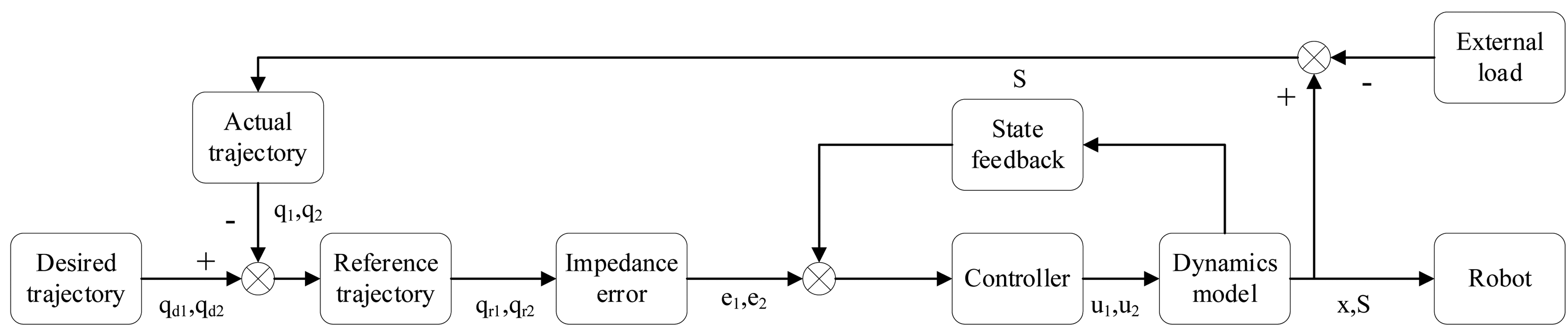
Schematic block diagram.

Singular perturbation control

Design of variable impedance controller

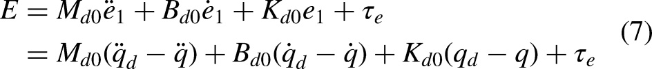
Impedance error, the deviation between actual and desired impedance, affects the accuracy and reliability of robotic control systems. Impedance control requires real-time feedback on forces and positions to adjust parameters and ensure proper interaction. However, environmental complexity and uncertainty often cause discrepancies, leading to oscillations or overshoots in rehabilitation scenarios, which reduce control precision and system robustness. Sets the impedance error E:

\begin{aligned} E & = M_{d 0} {\ddot{e}}_{1} + B_{d 0} {\dot{e}}_{1} + K_{d 0} e_{1} + τ_{e} \\ = M_{d 0} ({\ddot{q}}_{d} - \ddot{q}) + B_{d 0} ({\dot{q}}_{d} - \dot{q}) + K_{d 0} (q_{d} - q) + τ_{e} \end{aligned}

(7)

Among them

M_{d 0}

B_{d 0}

and

K_{d 0}

in particular, the desired inertia matrix, damping matrix and stiffness matrix.

Define the reference trajectory $q_{r} \in R^{2}$ :

{\ddot{q}}_{r} + M_{d 0}^{- 1} B_{d 0} {\dot{q}}_{r} + M_{d 0}^{- 1} K_{d 0} q_{r} = ξ

(8)

Among them,

ξ = {\ddot{q}}_{d} + M_{d 0}^{- 1} (B_{d 0} {\dot{q}}_{d} + K_{d 0} q_{d} + τ_{e})

u = u_{s} + u_{f} = u_{s} + K_{θ} (\dot{θ} - \dot{q})

(9)

Among them, u is the control variable, specifically representing the joint torque input from the motor.

u_{s}

denotes the input moment of a slowly varying stiffness system, while

u_{f}

represents the input moment of the rapidly varying elastic system. The matrix

K_{θ}

is a diagonal positive definite matrix.

Assuming that $z = K (θ - q)$ , it follows that:

z + τ_{e} = M (q) \ddot{q} + C (q, \dot{q}) \dot{q} + G (q) + d (t)

(10)

B \ddot{z} + K_{θ} \dot{z} + K z = K (u_{s} (t) - B \ddot{q})

(11)

Where d(t) is a random perturbation.

Singular perturbation method

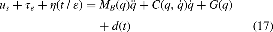
The core of singular perturbation method lies in adding a correction term to the rigid system in order to improve the inherent chattering phenomenon.²⁵

In the mathematical model of the flexible rehabilitation robot, it can be formulated into a fast time scale subsystem at the actuator and a quasi-steady state subsystem, that is, the fast-varying flexible part and the slow-varying rigid part are controlled by controllers respectively.²⁶

Assumptions K and $o (1 / ε^{2})$ is an equivalent infinitesimal, $K_{θ}$ and $o (1 / ε)$ is an equivalent infinitesimal; it can be rewritten as follows, here, $K_{1}$ and $K_{2}$ are equivalent infinitesimals of $o (1)$ :

K = \frac{K_{1}}{ε^{2}}, K_{θ} = \frac{K_{2}}{ε}

(12)

When

ε = 0

\bar{z} = {\bar{u}}_{s} - B \bar{\ddot{q}}

(13)

By Tikhonov's theorem,

z (t)

and

q (t)

respectively satisfy the formula (14), (15):

z (t) = \bar{z} (t) + η (T) + o (ε)

(14)

q (t) = \bar{q} (t) + o (ε)

(15)

Among them,

T = t / ε

is a rapidly changing time constant,

η

is the fast time variable. When

ε \to 0, T \to \infty

, the following boundary equations are satisfied:

B \frac{d^{2} η}{d T^{2}} + K_{1} η + K_{2} \frac{d η}{d T} = 0

(16)

By formula (16), The following formula can be obtained:

u_{s} + τ_{e} + η (t / ε) = M_{B} (q) \ddot{q} + C (q, \dot{q}) \dot{q} + G (q) + d (t)

(17)

B \frac{d^{2} η}{d T^{2}} (t / η) + K_{η} (t / η) + K_{θ} \frac{d η}{d T} (t / η) = 0

(18)

e_{2} = {\dot{e}}_{1} + k_{1} e_{1}

(19)

Where k₁ is a control parameter,

e_{1}

is is the error between q and

q_{r}

by formula (16), (19).

A slow subsystem control is available:

u_{s} = k_{2} e_{2} + M_{B} (q) ({\ddot{q}}_{r} + k_{1} e_{1}) + G (q) + C (q, \dot{q}) (\dot{q} + e_{2}) - τ_{e} + d (t)

(20)

Where k₂ is a control parameter. So the available controller:

\begin{aligned} u = k_{2} e_{2} + M_{B} (q) ({\ddot{q}}_{r} + k_{1} e_{1}) + G (q) + C (q, \dot{q}) (\dot{q} + e_{2}) \\ - τ_{e} + d (t) - K_{θ} (\dot{θ} - \dot{q}) \end{aligned}

(21)

By formula (20),

M_{B} (q) {\dot{e}}_{2} = - C (q, \dot{q}) e_{2} - k_{2} e_{2} - η (t / ε)

(22)

Stability analysis

To verify the stability of the variable impedance controller that was designed using the singular perturbation method, a Lyapunov function is designed. The convergence of the impedance error E is confirmed by applying the Lyapunov theorem. This process validates the robustness of the closed-loop system of the designed impedance controller.

We make the assumption that the dynamic equation of the series elastic actuator is set as (5), (6). Designing variable impedance controller inputs $u (t)$ as shown in the formula (21) So when $t \to \infty$ , $e_{2}$ and $η$ tends to 0, further proving the convergence of the impedance error e.

Definition $x = [η^{T}, {\dot{η}}^{T}]^{T}$ , by (19), it follows that:

\dot{x} = A x

(23)

There,

A = [\begin{matrix} 0 & I \\ - B^{- 1} K & - B^{- 1} K_{θ} \end{matrix}]

(24)

Because

| λ I - A | = | λ^{2} I + B^{- 1} K_{θ} λ + B^{- 1} K |

, and B, K,

K_{θ}

is a diagonal positive definite matrix, so the eigenvalues of A are negative. Given a matrix H, there exists a matrix D, and both H and D are diagonal positive definite matrices, satisfying the following formula:

A^{T} D + D A = - H

(25)

Design the Lyapunov function as follows,

V_{1} = \frac{1}{2} e_{2}^{T} M_{B} (q) e_{2} + \frac{1}{2} x^{T} D x

(26)

Because

{\dot{M}}_{B} (q) - 2 C (q, \dot{q})

is a skew-symmetric matrix and

M_{B} (*) = M (*) + B

where B is a constant matrix, so

e_{2}^{T} ({\dot{M}}_{B} (q) - 2 C (q, \dot{q})) e_{2} = 0

, so the formula (26) can be written as:

{\dot{V}}_{1} = - k_{2} e_{2}^{T} e_{2} - e_{2}^{T} η - x^{T} H x

(27)

By Young's inequality:

| e_{2}^{T} η | \leq \frac{1}{2 ξ} e_{2}^{T} e_{2} + \frac{ξ}{2} η^{T} η

(28)

For an arbitrary

ξ > 0

are established.

According to the formula (27), (28), It can be further obtained that,

{\dot{V}}_{1} \leq - {\bar{k}}_{2} e_{2}^{T} e_{2} - k_{h} x^{T} x \leq k_{v} V_{1}

(29)

Among them,

\begin{aligned} {\bar{k}}_{2} = k_{2} = - \frac{1}{2 ξ}, k_{h} = λ_{min} {H} - \frac{1}{2 ξ}, \\ k_{v} = min {\frac{2 k_{h}}{λ_{min} (D)}, \frac{2 {\bar{k}}_{2}}{λ_{max} (M_{B} (q))}} \end{aligned}

(30)

Where the control parameters satisfy

{\bar{k}}_{2} > 0

k_{v} > 0

k_{h} > 0

According to Lyapunov's theorem, the convergence of $V_{1}$ can be obtained, so we can conclude that $e_{2}$ and $η$ are convergent. Formula (22) shows that the convergence of $e_{2}$ and $η$ ensures the convergence of ${\dot{e}}_{2}$ . Additionally, since $e_{2}$ and ${\dot{e}}_{2}$ converge to 0, it can be concluded that at $t \to \infty$ , $e_{1}$ , ${\dot{e}}_{1}$ and ${\ddot{e}}_{1}$ all converge, thereby demonstrating the convergence of the impedance error E.

Optimal stiffness control strategy

In order to improve the effectiveness of rehabilitation robot-assisted rehabilitation therapy, the robot controller should encourage the active participation of the patient. At the same time, if the patient's movement deviates from the desired movement, it needs to be restrained. Therefore, the stiffness of the rehabilitation robot needs to be set in a reasonable range. To balance patient engagement and trajectory offset error, set the reward function:

r = a_{1} F_{h} V - | | a_{2} e | |^{2} = (a_{1} F_{x} V_{x} - a_{x}^{2} e_{x}^{2}) + (a_{1} F_{y} V_{y} - a_{y}^{2} e_{y}^{2})

(31)

Where

F_{h} V

is the patient's output power, which measures the patient's effort,

e_{x}

e_{y}

is the trajectory error in the terminal Cartesian space,

a_{1}

a_{2}

is a parameter that balances patient effort and trajectory offset.

Let $K_{h}$ be the estimated stiffness of the human upper limb end and $K_{r}$ be the stiffness of the impedance controller of the rehabilitation robot.

{\begin{matrix} F_{x} = K_{h x} (x_{d} - x) - B_{h x} V_{x} \\ F_{y} = K_{h y} (y_{d} - y) - B_{h y} V_{y} \end{matrix}

(32)

r = (K_{h x} e_{x} V_{x} - a_{1} B_{h x} V_{x}^{2} - a_{x}^{2} e_{x}^{2}) + (K_{h y} e_{y} V_{y} - a_{1} B_{h y} V_{y}^{2} - a_{y}^{2} e_{y}^{2})

(33)

In order to maximize the reward function,

\frac{δ r}{δ e_{x}} = 0

\frac{δ r}{δ e_{y}} = 0

{\begin{matrix} {\hat{e}}_{x} = \frac{a_{1} K_{h x} V_{x}}{2 a_{2}^{2}} \\ {\hat{e}}_{y} = \frac{a_{1} K_{h y} V_{y}}{2 a_{2}^{2}} \end{matrix}

(34)

During rehabilitation training, the robot's inertia, acceleration, and velocity are minimal, allowing for the neglect of inertia and Coriolis forces. Additionally, friction forces are negligible compared to joint torques. Assuming the affected limb remains stable for a short time, the robot's force equals that of the patient. The optimal stiffness for impedance control can then be determined as follows.

{\begin{matrix} {\hat{K}}_{r x} = \frac{2 a_{2}^{2} (B_{r x} + B_{h x})}{a_{1} K_{h x}} \\ {\hat{K}}_{r y} = \frac{2 a_{2}^{2} (B_{r y} + B_{h y})}{a_{1} K_{h y}} \end{matrix}

(35)

The optimal stiffness values

{\hat{K}}_{r x}

{\hat{K}}_{r y}

for impedance control maximize the reward function during rehabilitation training. As shown in Equation (37), the robot's optimal stiffness is inversely proportional to the affected limb's stiffness, aligning with the assist-as-needed principle: as the limb's ability decreases, the robot's assistance increases. A larger

a_{1}

parameter results in smaller robot stiffness, emphasizing the limb's effort in rehabilitation. Stiffness is positively correlated with the robot's assistance level.

When the affected limb is highly impaired $(K_{h x} \approx 0, K_{h y} \approx 0)$ , the robot's stiffness tends toward infinity. To prevent this, minimum $(K_{min})$ and maximum $(K_{max})$ stiffness limits are set for the impedance control.

K_{r} = max {K_{min}, min {K_{max}, {\hat{K}}_{r}}}

(36)

Simulation experiment

Establishment of the simulation model

To demonstrate the effectiveness of the proposed algorithm, simulation experiments were conducted to verify the singular perturbation method based on stability analysis, as depicted in Figure 6. A Simulink simulation model based on SEA was constructed for this purpose. It primarily consists of the desired trajectory of the two joints, the reference trajectory, the impedance error, the control input for the two joints, the dynamic model of the SEA, and the clock signal.

Simulation results

Torque control simulation

In practical rehabilitation robot applications, human-robot interaction forces often vary. Thus, our goal is to evaluate the controller's ability to balance trajectory tracking performance and steady-state error in the presence of disturbance forces, as well as its adaptability to external load forces. To achieve this, output and error performance are tested under varying external interaction forces. In the MATLAB/Simulink simulation model, sinusoidal loads with frequencies of $1 / π$ and amplitudes of 0.5 N, 1 N, and 2 N are introduced, while impedance parameters and desired positions remain constant. This simulates different external input torque conditions while keeping impedance and position unchanged. The simulation parameters are set as follows Table 1:

Table 1

Torque control simulation parameter setting.

Parameter	Value
External load 0.5 N	$f_{e 1} = 0.5 \sin (2 t), f_{e 2} = 0.5 \cos (2 t)$
External load 1 N	$f_{e 1} = \sin (2 t), f_{e 2} = \cos (2 t)$
External load 2 N	$f_{e 1} = 2 \sin (2 t), f_{e 2} = 2 \cos (2 t)$
Desired impedance M_d	$M_{d} = I_{2 \times 2}$
Desired impedance B_d	$B_{d} = I_{2 \times 2}$
Desired impedance K_d	$K_{d} = 50 I_{2 \times 2}$
Desired trajectory q	$q_{d 1} = 1, q_{d 2} = 1$

To compare the variable impedance control system with the traditional PD controller, the latter is implemented in the original model. Performance is evaluated using key indicators to assess their differences. The robot's dynamic and kinematic parameters remain unchanged. The PD controller parameters were optimized using MATLAB self-tuning for optimal performance, and adjusted based on the robot's actual motion to achieve smoother, more stable behavior. For Joint 1, the PD parameters are K_p = 5.355 and K_d = 4.631, for Joint 2, K_p = 4.768 and K_d = 2.739. The simulation results are as follows:

Figures 8 and 9 show the motion of the two joints under sinusoidal external load forces with both controllers. In these figures, the dash-dotted line represents a 0.5 N load, the solid line represents 1 N, and the dashed line represents 2 N.

Figure 7 illustrates the joint trajectories with the variable impedance controller. The motion remains relatively stable as external load forces increase. Joint 1's trajectory stays near 0.95 rad, fluctuating by about 0.1 rad, with a maximum deviation of 0.14 rad. Similarly, joint 2's trajectory remains stable around 0.95 rad, with fluctuations increasing to a maximum of 0.16 rad.

Figure 7

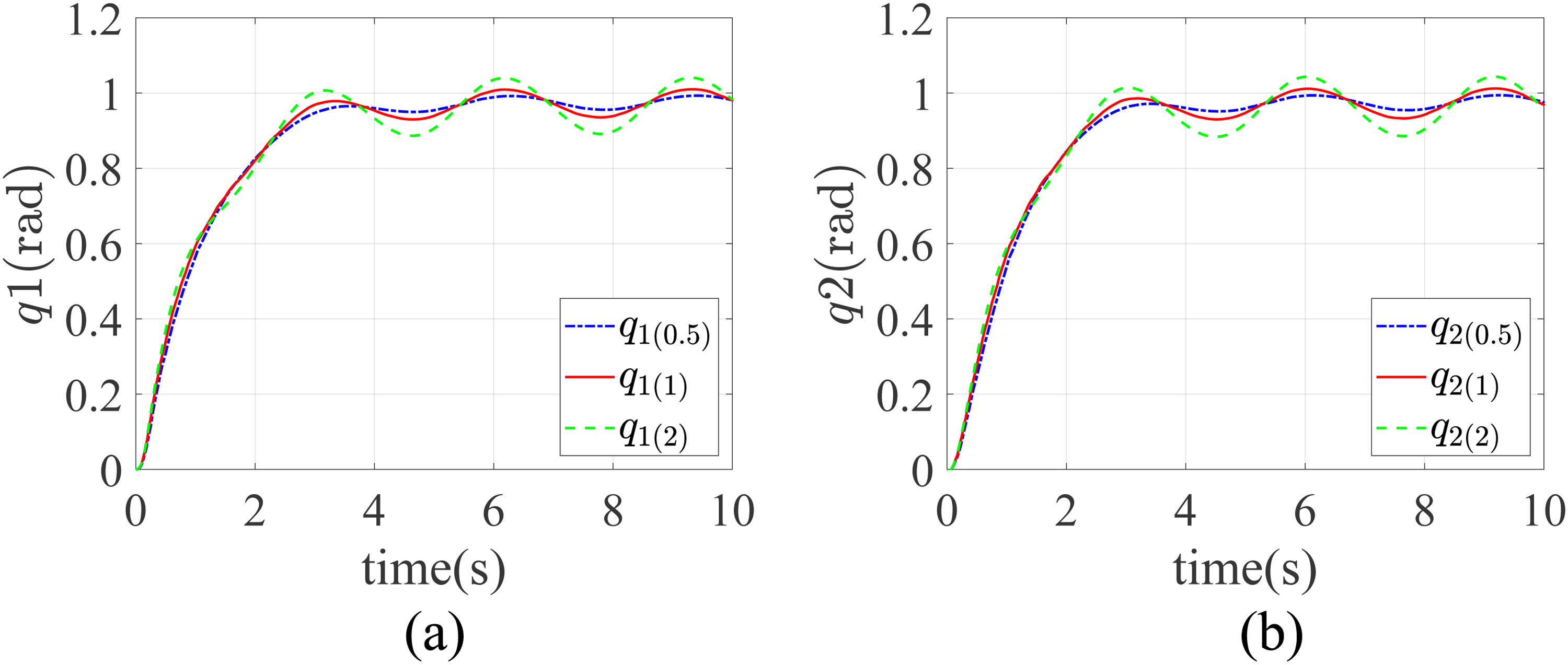
Joint trajectory under the variable impedance controller. (a) Actual trajectory of joint 1 (b) Actual trajectory of joint 2.

Figure 8 shows the motion under the PD controller. While the trajectory remains largely unchanged with increasing external load, the PD controller exhibits larger deviations compared to the variable impedance controller. Joint 1's trajectory stabilizes at around 0.8 rad, with fluctuations increasing by approximately 0.1 rad, reaching a maximum of 0.18 rad. Joint 2's trajectory also stays around 0.8 rad, with fluctuations increasing by 0.1 rad as the load force rises.

Figure 8

Joint trajectory under the PD controller. (a) Actual trajectory of joint 1 (b) Actual trajectory of joint 2.

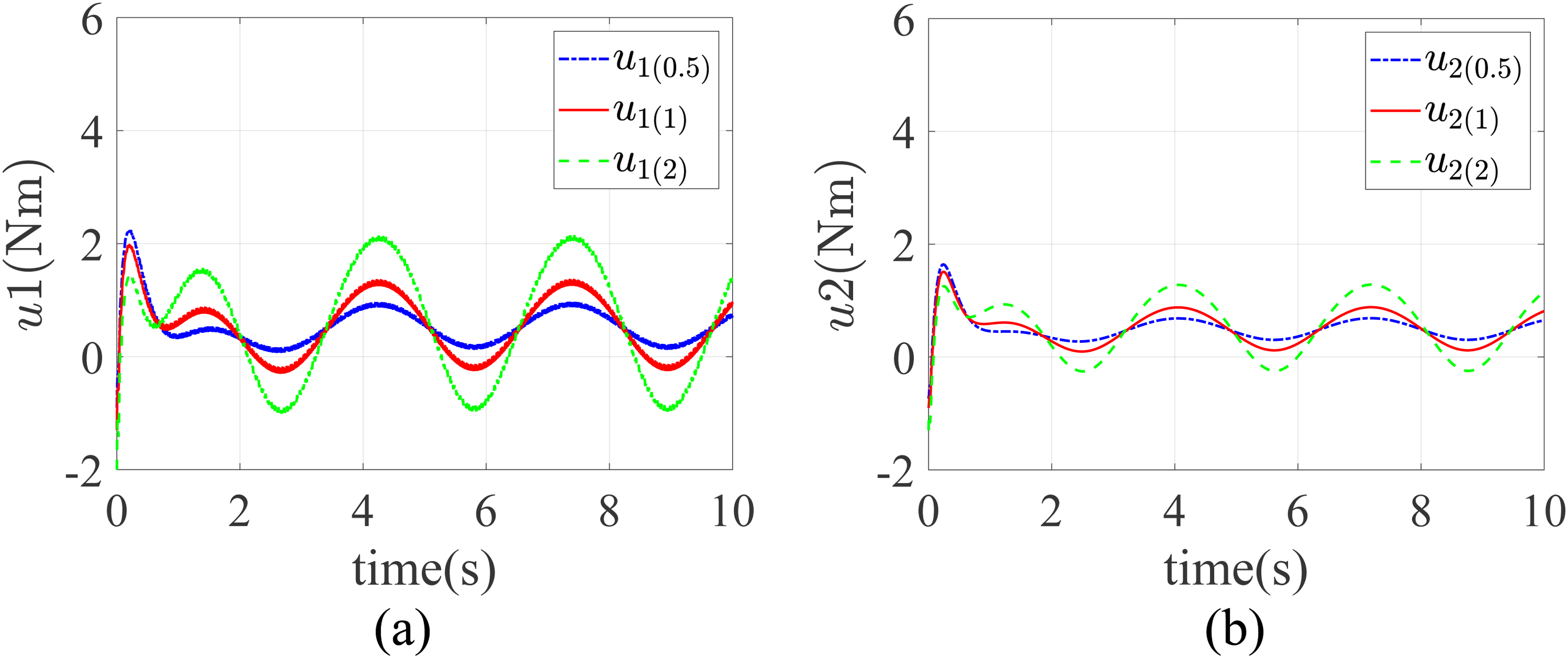
Figures 9 and 11 show the output torque of the two joints under both controllers. The dash-dotted line represents 0.5 N load, the solid line represents 1 N, and the dashed line represents 2 N load.

Figure 9

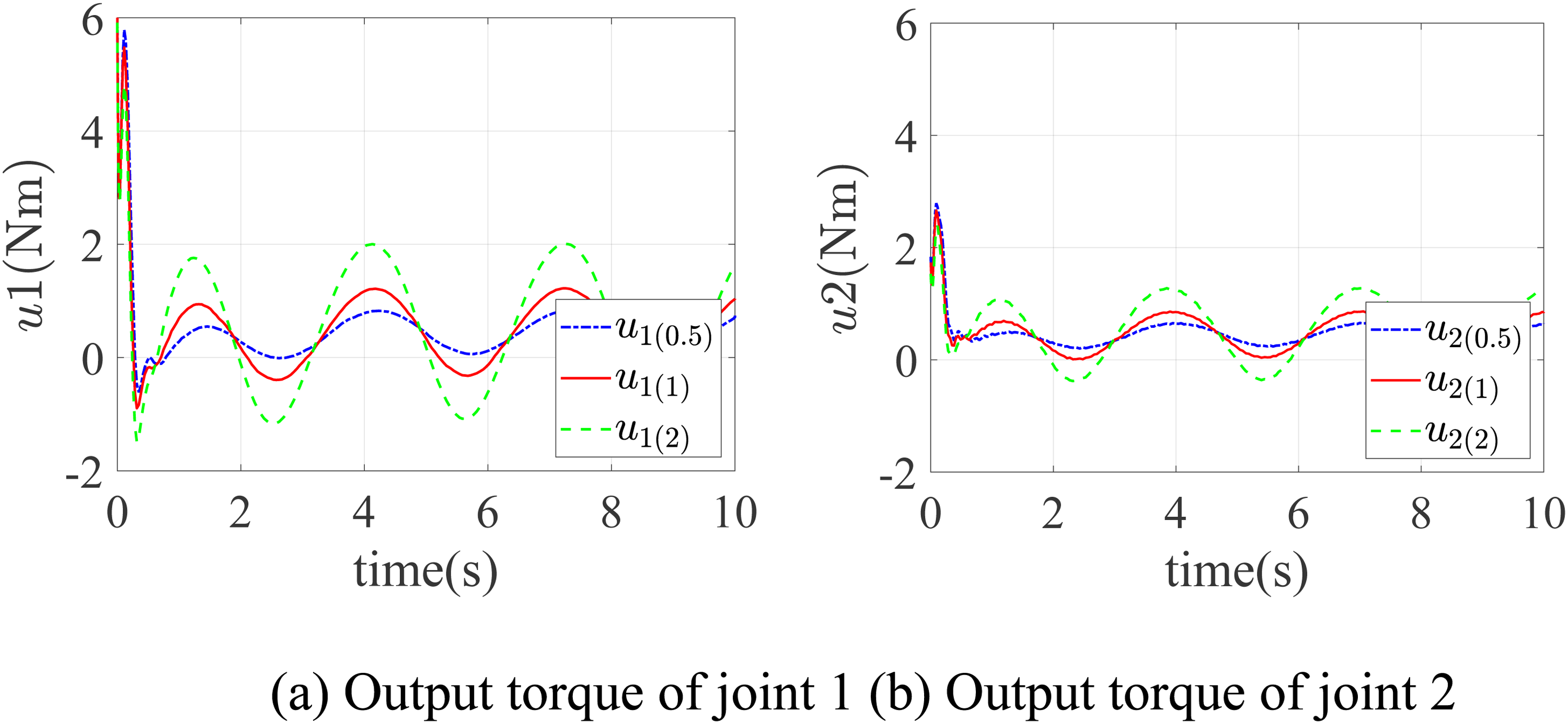
The output torque of joints under the variable impedance controller. (a) Output torque of joint 1 (b) Output torque of joint 2.

Figure 10 illustrates the variable impedance controller's effect. The output torque increases rapidly within the first 0.5 s, then stabilizes, with torque rising as external load forces increase. Joint 1 exhibits higher torque than joint 2, in line with the robot's actual structure. This confirms that the output torque responds to external load forces, validating the torque control and position-holding functions.

Figure 10

The output torque of joints under the PD controller. (a) Output torque of joint 1 (b) Output torque of joint 2.

Figure 10 shows the PD controller's effect. Similar to the variable impedance controller, the output torque changes significantly in the first second before stabilizing, with torque increasing as external load forces rise. However, the PD controller's torque changes more gradually in the first second, requiring more time to reach a stable state.

Figure 11 compares the mean position error of the robot's two joints with the PD and variable impedance controllers under different sinusoidal load inputs. The position retention ability of the two controllers shows a clear performance gap. With the PD controller, joint 1 errors exceed 0.15 rad, and joint 2 errors exceed 2 rad. In contrast, both joints’ errors remain below 0.005 rad with the variable impedance controller.

Figure 11

The average position error. (a) Average position error of joint 1 (b) Average position error of joint 2.

These results demonstrate that the variable impedance controller, based on the singular perturbation method, offers superior torque control performance.

Variable impedance control simulation

In rehabilitation, robots must interact safely, comfortably, and effectively with patients. The robot's impedance parameters are critical for adapting interactions to different patients, rehabilitation stages, and treatment needs. Thus, evaluating the control system's ability to handle changes in impedance parameters is essential. To achieve this, set simulation parameters as follows Table 2:

Table 2

Variable impedance control simulation parameter setting.

Parameter	Value
External load f	$f_{e 1} = 0.5 \sin (0.5 t), f_{e 2} = 0.5 \cos (0.5 t)$
Desired impedance M_d	$M_{d} = I_{2 \times 2}$
Desired impedance B_d	$B_{d} (t) = diag (5 + \sin (t), 5 + \cos (t))$
Desired impedance K_d	$K_{d} (t) = diag (10 + \sin (t), 10 + \cos (t))$
Desired trajectory q	$q_{d 1} (t) = 0.5 + \cos (0.5 π t),$
Desired trajectory q	$q_{d 2} (t) = 0.5 + \sin (0.5 π t)$

By applying a sinusoidal load to the robot and adjusting impedance parameters accordingly, we simulate the dynamic interaction between the patient and robot during rehabilitation. This verifies the effectiveness of the variable impedance controller in adapting its control strategy to changing impedance parameters. The simulation results are as follows:

In Figure 12(a), the actual trajectories closely align with the expected trajectories for both joints using the variable impedance controller. In contrast, Figure 13(a) shows noticeable deviations between the expected and actual trajectories with the PD controller.

Figure 12

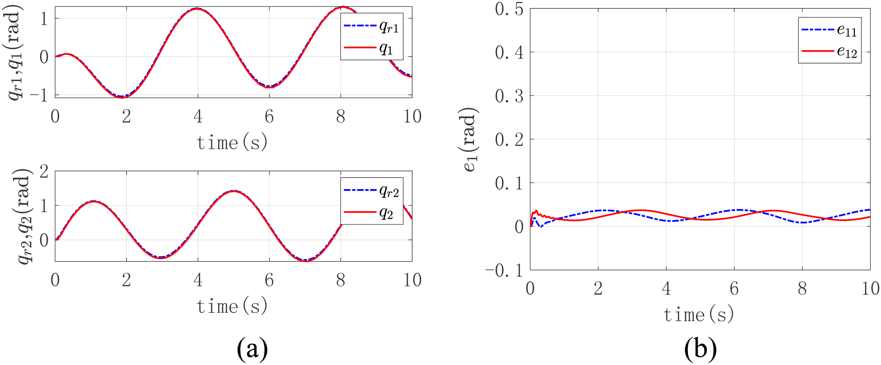
Joint trajectory and trajectory tracking error under the variable impedance controller. (a) Reference and actual trajectory (b) Reference trajectory tracking error.

Figure 13

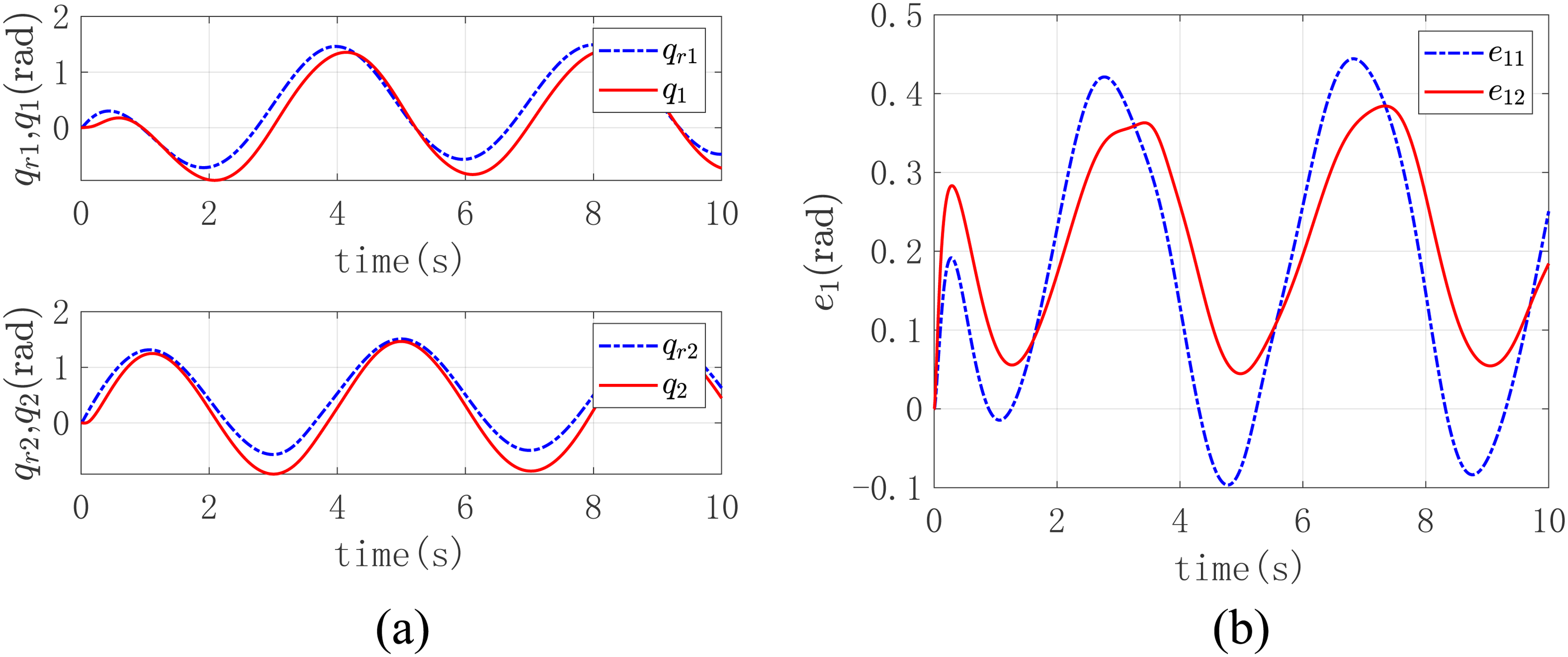
Joint trajectory and trajectory tracking error under the PD controller. (a) Reference and actual trajectory (b) Reference trajectory tracking error.

Figure 12(b) illustrates the reference trajectory tracking error $e_{1}$ with the variable impedance controller, demonstrating convergence to a near-zero equilibrium point with a steady-state error below 0.04. However, as shown in Figure 13(b), the PD controller results in significant trajectory tracking errors, with maximum errors of 0.38 rad for joint 1 and 0.45 rad for joint 2, without convergence.

Figure 13 shows the impedance error E for both joints under two controllers, with the dash-dotted line representing joint 1 and the solid line representing joint 2.

Figure 14(a) illustrates the impedance error variation under the variable impedance controller, where both joints’ errors converge within 0.5 s. The impedance error of joint 1 stabilizes within 0.3 Nm, and joint 2's error stays within 0.5 Nm. This confirms that the variable impedance controller effectively drives the error toward zero.

Figure 14

Variation of impedance error E under different controllers. (a) Variable impedance controller (b) PD controller.

In contrast, Figure 14(b) shows the impedance error under the PD controller, where the errors remain unstable. Joint 1's impedance error fluctuates between −3 Nm and 6 Nm, while joint 2's error oscillates between −1 Nm and 2.7 Nm, without converging to a stable value. Thus, the singular perturbation-based impedance control ensures convergence to the desired impedance dynamics, while the PD controller fails to achieve this stability.

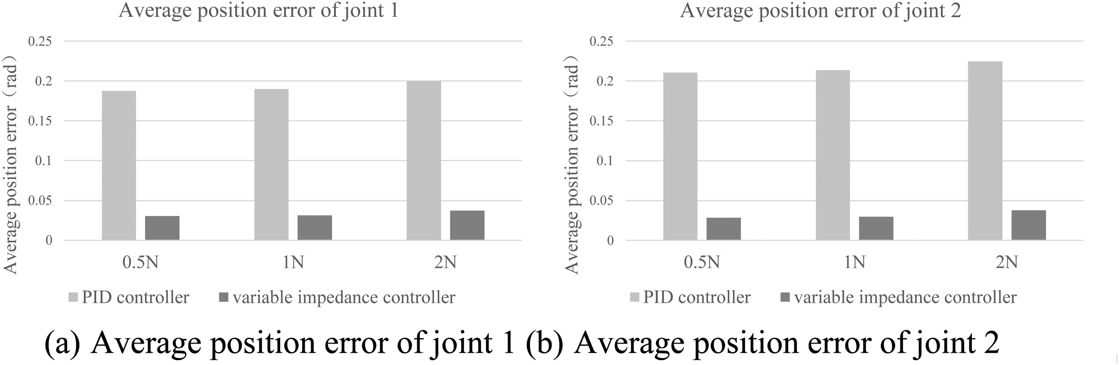
Figure 15 compares the mean impedance errors for the PD and variable impedance controllers. The dark cylinder represents joint errors under the variable impedance controller, while the light cylinder represents errors under the PD controller. The mean error for the PD controller is significantly higher, with joint 1 exceeding 1.8 rad and joint 2 above 1 rad. In contrast, the variable impedance controller keeps the errors below 0.3 rad for joint 1 and 0.2 rad for joint 2. Additionally, the impedance error of joint 1 is consistently higher, likely due to control error accumulation, as it is the terminal joint, influenced by joint 2's motion.

Figure 15

Average impedance error of the two controllers.

To assess the impact of impedance control on assist-as-needed strategies, demand-driven simulations were conducted in MATLAB/Simulink with consistent parameters. The experiments varied stiffness values (K_d = 0, 1, 10, 50, 100, 1000) over a 10-s simulation, with inertia M_d = 1 and damping B_d = 50.

Figure 16 shows position tracking errors, illustrating that higher stiffness (K_d) results in faster error convergence. When K_d = 0, convergence is minimal, demonstrating that higher stiffness improves position tracking performance.

Figure 16

Joint impedance error.

Based on the above experimental results, it can be demonstrated that the variable impedance controller using the singular perturbation method outperforms the traditional PD controller in controlling impedance dynamics.

Variable stiffness experiment

Experimental platform

To validate the proposed theory, a two-degree-of-freedom desktop rehabilitation robot based on SEA joints was constructed (Figure 17). This robot features two serially connected joints with a serial elastic actuator (SEA) linking them. Carbon fiber tubes connect the SEA joints and the end effector grip to the second SEA joint. A six-dimensional force sensor on the end effector base measures forces and torques in three Cartesian directions. A coordinate system is established at the center of the first SEA joint, focusing on the x and y directions for this desktop rehabilitation setup.

Figure 17

Experimental platform.

Experimental protocol

The adaptive impedance control experiment based on the assist-as-needed strategy is designed as follows: The task involves moving the patient's arm end effector from point A (0.5 m, 0) to point C (0.2 m, 0) within 10 s. A fifth-degree polynomial is used for x-direction trajectory planning, as shown in Figure 18(a). The position, velocity, and acceleration of the end effector are presented, with zero velocity and acceleration at both start and end points. This approach minimizes motor impact during startup and shutdown while ensuring a smooth trajectory for stable rehabilitation and better limb recovery. The desired joint trajectories, derived from inverse kinematics, are shown in Figure 18(b), with q1 and q2 as position control signals for the joint servos.

Figure 18

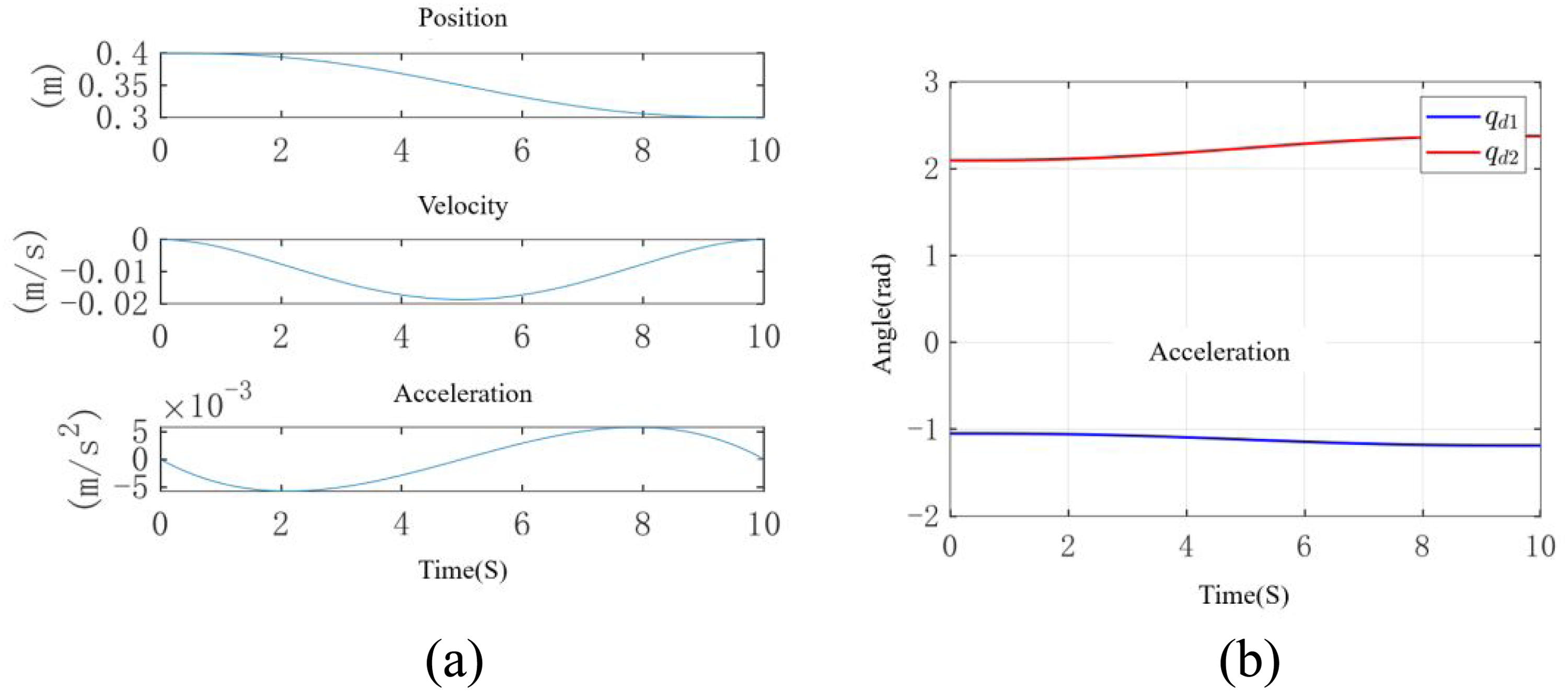
Assist-as-needed strategy trajectory planning. (a) Trajectory planning (x) (b) Desired trajectories.

Experimental result

The experimental parameters were set to prioritize the human upper limb's work in the rehabilitation strategy. The optimal stiffness limits were defined as K_max = 400 N/m and K_min = 10 N/m, ensuring safety by protecting the affected limb. The results include the end effector trajectory, human-robot interaction forces, identified damping, upper limb stiffness, and the robot's optimal stiffness under the assist-as-needed strategy.

As illustrated in Figure 19, during the rehabilitation training process, an increase in the damping and stiffness exhibited by the patient's upper limb corresponds to a decrease in the robot's optimal stiffness. This indicates a lower level of assistance provided by the robot, which aligns with the principles of assist-as-needed in rehabilitation training. Thus, this observation validates the effectiveness of the assist-as-needed strategy.

Figure 19

Assist-as-needed strategy experiment results.

Conclusions

This paper presents a variable impedance controller for flexible joints based on the singular perturbation method. The controller is designed using Tikhonov's theorem to ensure the convergence of impedance error, and its stability is validated with the Lyapunov theorem. Simulation results demonstrate excellent response performance and position tracking. Compared to the PD controller, the proposed controller shows superior torque control under external loads and better variable impedance modulation. Future work will explore its application in multi-degree-of-freedom robotic arms and more complex human-robot interactions.

However, there are several limitations: (1) the robot model does not fully capture the interaction between the rehabilitation robot and the environment, leading to impedance discrepancies; (2) the singular perturbation method performs well at higher stiffness but needs further development for lower stiffness scenarios; (3) experiment parameters were designed to validate the control algorithm, not reflect actual patient movement during rehabilitation; (4) the validation on the physical platform is limited, requiring more extensive testing to assess stability and effectiveness.

Footnotes

Declaration of conflicting interests

The authors declared no potential conflicts of interest with respect to the research, authorship, and/or publication of this article.

Funding

The author(s) disclosed receipt of the following financial support for the research, authorship, and/or publication of this article: This work was supported by the National K&D Program of China (2022YFC3601400); Shanghai 2022 “Science and Technology Innovation Action Plan” biomedical science and technology support project (22S31901400).

ORCID iDs

Bingshan Hu

Hao Ren

Hongliu Yu

Data Availability Statement

Example text of a Data statement, as provided by the author.

References

Nagappan

Chen

Wang

. Neuroregeneration and plasticity: a review of the physiological mechanisms for achieving functional recovery postinjury. Military Med Res 2020; 7: 16. Review.

Gull

Bai

Bak

. A Review on Design of Upper Limb Exoskeletons. Robotics 2020; 9: 16. Doi:https://doi.org/10.3390/robotics9010016

Heng

Solomon

Gao

. Flexible Electronics and Devices as Human-Machine Interfaces for Medical Robotics. Advanced Materials 2022; 34: 16. DOI: https://doi.org/10.1002/adma.202107902

Sanchez

Walsh

Wood

. Textile Technology for Soft Robotic and Autonomous Garments. Advanced Functional Materials 2021; 196: 113960. DOI: https://doi.org/10.1002/adfm.202008278

Trigili

Crea

Moisè

, et al. Design and experimental characterization of a shoulder-elbow exoskeleton with compliant joints for post-stroke rehabilitation. Ieee-Asme Transactions on Mechatronics 2019; 24: 1485–1496.

Koo

Chang

Sohn

, et al. Shoulder mechanism design of an exoskeleton robot for stroke patient rehabilitation. In: 2011 IEEE International Conference on Rehabilitation Robotics , 2011, 29 June–1 July 2011, pp.1–6.

Gopura

Kiguchi

, et al. SUEFUL-7: a 7DOF upper-limb exoskeleton robot wlith muscle-model-oriented EMG-based control. In: IEEE RSJ International Conference on Intelligent Robots and Systems , St Louis, MO, 2009, Oct 10–15 2009, pp.1126–1131.

Varghese

Nguyen

Burdet

, et al. Nonlinearity compensation in A multi-DoF shoulder sensing exosuit for real-time teleoperation. In: 3rd IEEE International Conference on Soft Robotics (RoboSoft), New Haven, CT, Jul 15 2020, pp.668–675.

Nef

Guidali

Riener

. ARMin III - arm therapy exoskeleton with an ergonomic shoulder actuation. Appl Bionics Biomech (UK) 2009; 6: 127–142.

10.

Bardi

Gandolla

Braghin

, et al. Upper limb soft robotic wearable devices: a systematic review. Journal of Neuroengineering and Rehabilitation 2022; 19: 87. DOI: https://doi.org/10.1186/s12984-022-01065-9

11.

Pont

Contreras

Samper

, et al. Exoflex: an upper-limb cable-driven exosuit. In: Robot 2019: Fourth Iberian Robotics Conference , 2020 (ed Silva

Luís Lima

Reis

, et al.), 2020, pp.417–428: Cham: Springer International Publishing.

12.

Maciejasz

Eschweiler

Gerlach-Hahn

, et al. A survey on robotic devices for upper limb rehabilitation. Journal of Neuroengineering and Rehabilitation 2014; 11: 3. DOI: https://doi.org/10.1186/1743-0003-11-3

13.

Vatan

HMF

Nefti-Meziani

Davis

, et al. A review: A Comprehensive Review of Soft and Rigid Wearable Rehabilitation and Assistive Devices with a Focus on the Shoulder Joint. Journal of Intelligent & Robotic Systems 2021; 102: 415. DOI: https://doi.org/10.1007/s10846-021-01353-x

14.

Abu-Dakka

Saveriano

. Variable Impedance Control and Learning-A Review. Frontiers in Robotics and Ai 2020; 7: 590681. DOI: https://doi.org/10.3389/frobt.2020.590681

15.

Brahmi

Driscoll

El Bojairami

, et al. Novel adaptive impedance control for exoskeleton robot for rehabilitation using a nonlinear time-delay disturbance observer. Isa Transactions 2021; 108: 381–392.

16.

Albu-Schäffer

Ott

Hirzinger

. A unified passivity based control framework for position, torque and impedance control of flexible joint robots. In: Thrun

Brooks

Durrant-Whyte

(eds) Robotics research. Berlin, Heidelberg: Springer, 2007, pp.5–21.

17.

Liu

. Iterative learning impedance control for rehabilitation robots driven by series elastic actuators. Automatica 2018; 90: 1–7.

18.

Sharifi

Behzadipour

Salarieh

, et al. Cooperative modalities in robotic tele-rehabilitation using nonlinear bilateral impedance control. Control Engineering Practice 2017; 67: 52–63.

19.

Zhou

Wang

, et al. A hybrid control strategy for grinding and polishing robot based on adaptive impedance control. Advances in Mechanical Engineering 2021; 13. DOI: https://doi.org/10.1177/16878140211004034

20.

Sun

. Adaptive impedance control of robots with reference trajectory learning. IEEE Access 2020; 8: 104967–104976.

21.

Deng

Sun

Guo

, et al. Singular perturbation-based Variable impedance control of robots with series elastic actuators. In: 38th Chinese Control Conference (CCC) , 2019, Guangzhou, PEOPLES R CHINA, Jul 27–30 2019, pp.4397–4402.

22.

Kronander

Billard

. Stability considerations for Variable impedance control. Ieee Transactions on Robotics 2016; 32: 1298–1305.

23.

Liang

Wang

Zhong

, et al. Robust Variable Impedance Control for Aerial Compliant Interaction With Stability Guarantee. Ieee Transactions on Industrial Informatics 2023; 20: 3351–3360. DOI: https://doi.org/10.1109/tii.2023.3306574

24.

Gosselin

Nguyen

. On the stability of macro-mini robotic systems for physical human-robot interaction. Mechanism and Machine Theory 2023; 185: 3398–3409. DOI: https://doi.org/10.1016/j.mechmachtheory.2023.105304

25.

Che

Mobayen

, et al. A Singular Perturbation Approach-Based Non-Cascade Sliding Mode Control for Surface-Mounted PMSMs. Appl Sci-Basel 2022; 12: 20. DOI: https://doi.org/10.3390/app122010500

26.

Yang

. On the singularly perturbation fractional kirchhoff equations: critical case. Advances in Nonlinear Analysis 2022; 11: 1097–1116.

Research on variable impedance control of SEA-driven upper limb rehabilitation robot based on singular perturbation method

Abstract

Keywords

Introduction

Flexible two-degree of freedom robot system

Kinematics model

Dynamics model

Singular perturbation control

Design of variable impedance controller

Singular perturbation method

Stability analysis

Optimal stiffness control strategy

Simulation experiment

Establishment of the simulation model

Simulation results

Torque control simulation

Variable impedance control simulation

Variable stiffness experiment

Experimental platform

Experimental protocol

Experimental result

Conclusions

Footnotes

Declaration of conflicting interests

Funding

ORCID iDs

Data Availability Statement

References