Sage Journals: Discover world-class research

Abstract

The presented research investigates the accuracy of a localization algorithm using lidar (NAV-350) pose data in a GPS denied environment. A template matching solution is presented using the corners of the workspace area as markers. Results are also compared against the lidar NAV-350's own software solution which are based on average reflector distance. The presented algorithm has shown to have a higher accuracy in most cases. Data is analyzed for approximately 100 different locations in a workspace of 8.9 m by 10.7 m using an industry standard forklift with a base dimension of 1 m × 1.3 m. This paper shows how the algorithm can successfully determine the x, y coordinates and heading angle of the forklift in real time.

Keywords

Forklift localization position tracking template matching neural network

Introduction

Autonomous mobile robots (AMRs) are riding a prosperous market due to multinational manufacturers who are successfully including them in their warehouse automation plans. Especially because of the trend of Industry 4.0, the concept of autonomous forklift vehicles in real factory environments is of particular interest to researchers. Modern facilities are attracted by this digital trend as it increases the technological intelligence in the manufacturing industry. This leads to more efficient labor distribution and novel infrastructure design of industrial autonomous systems and automated warehouse management.¹ In this respect, a particular area of interest is in the navigation or localization of the forklift. Researchers have already shown success in path planning strategies. For small freight, they have used the shortest path algorithm and A* algorithm based on vision.² There is also published work on robotic forklifts for intelligent warehouse, but it has not been experimentally validated with multiple forklifts.³ Research has been published on time-varying feedback control of unmanned autonomous industrial forklifts where sonar, laser range finder, etc. was used.⁴ The control algorithm in such research forced the forklift to travel on a trajectory given by a path planner. Past research using image-based approaches utilized specific features captured by camera to differentiate between the forklift's pallets and its environment.⁵ In other approaches, some used a radio frequency identification (RFID) tag, others used wireless sensors and laser pointers and also laser sensors to differentiate between the pallets and the environment.^6,7 Researchers have also used a combination of ultrasound chirp and RF.⁸ Indoor positioning is quite successful using ultra wide band (UWB) technology. Here multiple positioning markers with fixed coordinates are placed in specific locations and the timing of the pulses from these markers are used to calculate the three-dimensional position using the least square method.⁹

There are many other similar applications using UWB with accuracy of position at centimeter-level making it a very promising field of research.^10,11 However, it faces challenges from non-line-of-sight as well as attenuation of signal.^12,13 Using multiple integrated sensors with UWB has also produced promising results.¹⁴ One research claimed success using an integration of UWB anchors, IMU, and template matching algorithm, but the authors were able to achieve an error of 33.4 cm.¹⁵ Here the template matching involved recording an image (using a monocular camera) at a particular frame and then calculating the highest similarity of a rectangular area for the next frame to determine its position.

This research is aimed at minimizing errors in a part of the navigation process of an AMR, or to be more specific, the localization of a forklift. The scope of the research in this paper will be on the localization only. The environment for this navigation is expected to be similar to an industrial warehouse where the ground will be smooth, and the presence of moving people will make the mapping of the warehouse somewhat dynamic. The ability to correctly predict the vehicle's exact location for enabling error free automated navigation requires a large amount of data evaluation from the lidar. The real challenge lies here, and this research is aimed at solving this problem with a reduction in error compared to established methods and tools. The control algorithm will be responsible for reducing the position and heading error.

The next section discusses the “Conceptual settings” involved in location and mapping. The following two sections after that will explain the methodology through the “Experimental hardware setup” and the “Mathematical model for localization of the forklift.” This will be followed by the “Results and discussion” section which also includes comparisons to other work. The paper will then end with the “Conclusion” section which also addresses future work that can be pursued in this area.

Conceptual settings

Just as we need to understand our location before navigation, so too do mobile robots. To understand their process, a few introductory concepts must be addressed first. If a robot's location is given by a pair of coordinates (x, y), they can describe its relative location (from start position) or an absolute position. But in neither case can the robot's orientation be determined. For this reason, another parameter, θ, is necessary to express its facing direction. Now the Pose vector (x, y, θ) can be used as a data structure expressing all aspects of its localization. For a three-dimensional localization, the z-coordinate can be calculated using the transpose of the two-dimensional Pose. Some research on robot behavior successfully showed the location estimation without knowing the robot's exact pose, but its accuracy was limited.¹⁶ Mobile robot localization is the problem of determining a robot's pose relative to a given map of the environment. It is often called position estimation. The forklift's localization is an instance of the general localization problem, which is the most basic perceptual problem in robotics.

Mapping is a process of storing extracted environmental information in a data structure. This can be represented in 2D (easier to create and evaluate) or 3D form (increased accuracy). Computer vision solutions and robotics solutions have already been proposed over the years.^17,18 The robot can use the sensors to measure its relative bearing to a prominent landmark on the map. Another method is to create the map in the form of an occupancy grid. The grid contains information such as which regions are free, and which are occupied. The robot's sensors measure the directional bearing from the nearest occupied region. The hypothesis space is quite big with a very high number of variables (e.g., approximately 1015 variables with such a discrete technique) and the process is quite complex when neither the robot's location nor the map is known. It is necessary to measure the uncertainty associated with the estimation of the robot's location. A proven powerful technique such as the Bayesian filtering can also be used to calculate this associated uncertainty.¹⁹

In 2003, Carnegie Mellon's Groundhog was used to explore and generate a map of an abandoned coal mine with the intention of working and navigating in conditions that are too toxic. This was one of the main causes for an exponential growth in the demand for robot localization, and ever since then researchers have been interested in mobile robots trying to construct a map while traveling. Simultaneous localization and mapping (SLAM) algorithms have been successful in generating a map of uncharted territory and are used by self-driving cars, planetary rovers and UAVs and AUVs. The process of SLAM involves controls and sensor readings at specific times to compute an estimate of the robot's location and a map of its surrounding environment. Research over the years has shown different approaches in robot navigation using maps and SLAM methods using maps.^20,21 Some of these were topological and metric representations while others were probabilistic forms.^22,23 But most research faces challenges when the maps are for large areas, possibly due to computational demands and prohibitive uncertainties associated with this.

Experimental hardware setup

The forklift used in this research as shown in Figure 1 is a Xilin Counterbalanced Electric Stacker with a Load capacity of 1500 kg and an overall service weight of 2020 kg. The forklift also has a maximum lifting height of 3 m, and a turning radius of 1.75 m. It should be noted that the base dimension of the forklift is 1 m by 1.3 m and the workspace for this experiment was 10.7 m by 8.9 m as shown in Figure 2. The lidar sensor used in this experiment is SICK NAV-350 as shown in Figure 3.

Figure 1.

Xilin counterbalanced electric stacker.

Figure 2.

The workspace.

Figure 3.

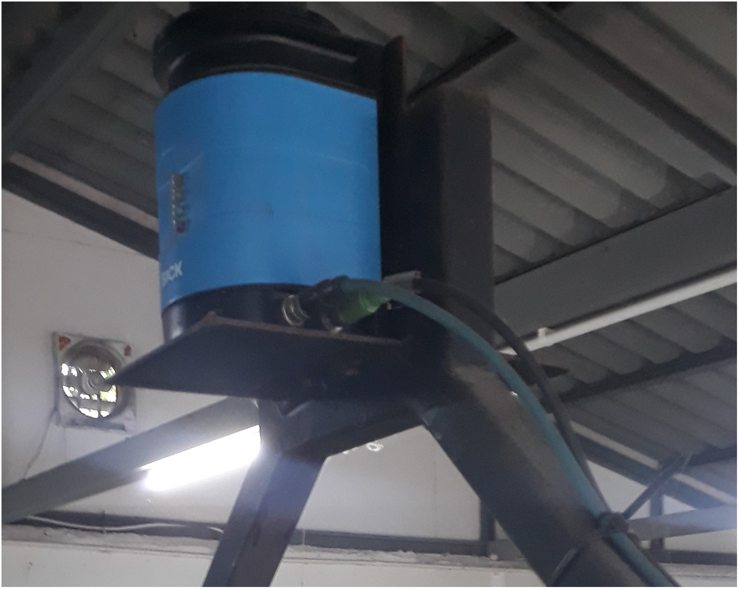
SICK NAV-350 lidar mounted on the forklift.

This is an indoor sensor that is mostly used with AGVs in determining their position using reflectors and its surrounding contour. It can extrapolate its own position (distance and angle) through a computer which can then be used to keep the AGV on course for a predetermined route.²⁴ Using a maximum of 36 W, the laser operates at the wavelength λ = 905 nm for a 360-degree scan angle. It can use up to 12,000 reflectors to determine its position although the device claims that a minimum of three reflectors is sufficient to ascertain its position and the accuracy of the device is reported to be dependent on its distance from the reflectors mounted on the walls of the workspace.²⁴

Mathematical model for localization of the forklift

The forklift's localization can be seen as a problem of coordinate transformation. Maps are described in a global coordinate system, which is independent of the forklift's pose. Localization is the process of establishing correspondence between the map coordinate system and the forklift's local coordinate system. Knowing this coordinate transformation enables the forklift to express the location of objects of interest within its own coordinate frame – a necessary prerequisite for its navigation. It is clear that knowing the pose x_t of the forklift is sufficient to determine this coordinate transformation, assuming that the pose is expressed in the same coordinate frame as the map.

x_{t} = (x y θ)^{T}

(1)

Unfortunately, herein lies the problem of all mobile robot localization. Usually, the pose cannot be sensed directly. Put differently, most robots do not possess a noise-free sensor for measuring their pose. The pose therefore must be inferred from data. A key difficulty arises from the fact that a single sensor measurement is usually insufficient to determine the pose. It will be assumed throughout the paper that the initial pose is known so the approach will basically be a position tracking algorithm on a static environment for passive localization. The approach will also include finding the position of the forklift on a geometric representation of the workspace (with walls as markers), or a model of the room to be more specific.

Suppose that a forklift moves within a room with straight walls. Then the lidar data will register each wall as a straight line in polar coordinates. Corners are then the intersection between such lines and introduce discontinuities into the data where one line becomes visible and the other becomes invisible. This simple process was not yielding the desired accuracy. Although most simulations yielded accuracy of around 5 cm, some were off by as much as 8 cm from the measured data. As the preliminary pose estimation needed to be refined, a few additional steps were required. Firstly, a reference room was applied, and the filtered data was projected back onto the raw data. After this, a local search was performed over the raw data to identify the corner coordinates. From the location of the corners, the pose could then be determined. After refining the initial pose estimation, many frames were aligned against a reference frame to gather statistics about the exact shape of the room. All the points were then statistically aggregated to compute a reference room, allowing any frame to be aligned to the room thereafter. Because the room is computed from many frames, the noise washes out errors in measurement. The uncertainty in this alignment then represents the uncertainty in the forklift's position.

In the following sections, a brief review of the relevant mathematics is given.

Mathematical descriptions of parameters used in algorithm

The detailed steps of the algorithm will be discussed in the “Data analysis” section and their corresponding effects will be shown in the “Results and discussion” section. A table showing the processing time for each step of the algorithm will be presented in Table 1. The major steps of the algorithm are:

Convert raw sensor data to usable form.

Discover the boundary and landmarks for the room from this data.

Create an aligned reference room from the sensor data as well as the room shape and size discovered by step 2.

As the forklift moved, new live data along with the results from step 3 were used to determine its current position with the help of a Neural Network classification as well as some statistical tools.

Table 1.

Processing cost time by each step of algorithm.

Step	Description	Duration
Radial filter	Process raw data	1.100e-03s
To cartesian	Change to Cartesian coordinates	1.294e-03s
Extract data	(optional step)	1.219e-06s
Angular align	Brute Force	1.339e+00s
Gradient angular align	Gradient Descent	2.354e-01s
Stochastic angular align	Stochastic Gradient Descent	4.253e-02s
Spatial align	Brute Force	8.693e+00s
Gradient spatial align	Gradient Descent	2.009e-01s
Stochastic gradient spatial align	Stochastic Gradient Descent	2.646e-02s

The rest of this section will focus on all relevant mathematical descriptions of the key parameters used in the algorithm.

Assume that a forklift is placed within a closed boundary that is denoted by B. The forklift's position is described by the vector $\vec{s}$ , which includes both position and rotation. The forklift then makes an angular scan of its environment. This scan is conducted in the forklift's frame of reference, called the robot frame, which is defined with the origin at the center of the forklift and with $\hat{x}$ pointing along the direction of the forklift's sensor in resting position. The scan begins at $\hat{x}$ and proceeds at regular angular intervals of size $Δ θ$ around the origin in the counterclockwise direction.

Δ θ = \frac{2 π}{N}

(2)

This scan produces a series of N measurements at angles

θ_{j} = j * Δ θ

where

j \in [0, 1, 2, \dots N - 1]

. Each measurement captures the distance from the forklift to the boundary in the direction of

θ_{j}

in the robot frame as seen in Figure 4.

Figure 4.

Schematic showing the coordinate systems.

The figure shows that the standard frame is the coordinate system centered at the middle of the room, with the x-axis as the horizontal line and the y-axis as the vertical line. The forklift is located by vector x, shown as the line running from the origin of the standard frame to the center of the forklift. The forklift is rotated at an angle $γ$ . The robot frame is shown with the origin at the center, and the x-axis tilted up by the angle $γ$ , and the y-axis tilted counterclockwise by the same angle $γ$ .

The scan captures the shape of the boundary of the room B as seen from the forklift's perspective from pose $\vec{s}$ (position and rotation). Since the scan is distance information (the distance from the forklift to the boundary at each angle $θ_{j}$ ) and since this data is in polar coordinates, the scan data is referred to as the radial data and written as:

r = r (θ) = r (θ, B) = r (θ, B, \vec{s})

(3)

The first equation

r = r (θ)

means that the data is most clearly understood as the radial information, taken in the robot frame, where

θ

is the angle from

\hat{x}

in the counter-clockwise direction in the robot frame and

r (θ)

is the distance from the center of the forklift (or the sensor) to the boundary B in the direction

θ

. The next equation

r (θ) = r (θ, B)

simply expresses the dependence of the radial data upon the shape of the room B. The final equation

r (θ, B) = r (θ, B, \vec{s})

emphasizes that the radial measurement depends also upon the forklift pose,

\vec{s}

(position and rotation).

If it is approximated that the forklift does not move throughout the duration of the scan, then this equation is written as:

r (j, t) = r (θ_{j}, \vec{s} (t))

(4)

The closed boundary B is omitted to avoid clutter. This equation says that the radial data at time t depends upon the forklift pose and the angle of the scan. The pose vector is written as

\vec{s} (t)

\vec{s} (t) = (\vec{x} (t), γ (t))

(5)

The relationship combines

\vec{x}

, the location of the center of the forklift, and its orientation

γ

, or the forklift's rotation.

To make these definitions a little clearer, the concept of standard orientation must be introduced. Standard orientation refers to the forklift in the center of the room with the sensor resting at $γ = 0$ . This frame of reference is convenient for aligning the forklift and for referencing the forklift's frame. For example, if the forklift moves to a position $\vec{x} = (2 m, 1.5 m)$ from the center and then the forklift rotates an angle $γ = π / 10$ , then the robot frame can be computed easily. Starting at the center of the room, move to $\vec{x} = (2 m, 1.5 m)$ , and then perform a rotation of $γ = π / 10$ . The forklift's first measurement will be at $θ = 0$ , which is measured in the forklift's frame and corresponds to $γ = π / 10$ in the room frame (but no longer in the standard orientation frame, since the origin has been translated) as seen in Figure 4.

When the forklift performs a scan and is not moving, or moving slow enough that its movement can be neglected over the duration of the scan, a series of data $\vec{r_{k}}$ can be obtained.

\begin{aligned} {\vec{r}}_{k} = & \vec{r} (t_{k}) \\ = & [r (θ_{0}, t_{k}), r (θ_{1}, t_{k}), r (θ_{2}, t_{k}), \dots, r (θ_{N}, t_{k})] \end{aligned}

(6)

Here the vector over the r, as in

\vec{r}

, denotes the entire series of measurements over the angular scan. When there is no vector over the r as in

r (θ_{0}, t_{k}) = r (θ_{j}, \vec{s} (t_{k}))

, then a single number, or a single distance from the forklift to the boundary B at angle

θ = θ_{0}

with the forklift at pose

\vec{s} = \vec{s} (t_{k})

is indicated.

The goal of the analysis is to determine the pose of the forklift 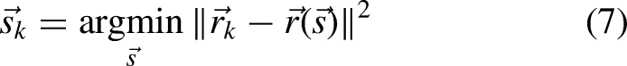$\vec{s}$ from the radial data $\vec{r}$ . If the boundary B is known, then $\vec{r} (\vec{s}, B)$ can be computed over different orientations $\vec{s}$ . In this manner, the pose estimation can be written as an optimization problem of the form:

{\vec{s}}_{k} = \underset{\vec{s}}{argmin} ‖ {\vec{r}}_{k} - \vec{r} (\vec{s}) ‖^{2}

(7)

This equation means that the orientation

\vec{s_{k}}

that minimizes the error function

‖ \vec{r_{k}} - \vec{r} (\vec{s}) ‖

must be solved for, which is simply the Euclidean norm of the difference between the two radial scans: the data

\vec{r_{k}}

and

\vec{r} (\vec{s})

, the computed or simulated measurement at the simulated position

\vec{s}

. The Euclidean norm is given as:

‖ \vec{r_{k}} - \vec{r} (\vec{s}) ‖^{2} = \sum_{j = 0}^{N - 1} [r_{k} (θ_{j}) - r (θ_{j}, \vec{s_{k}})]^{2}

(8)

Viewed as an optimization problem, this problem is challenging for two reasons: (a) the target function is non-linear and non-convex and (b) the space of possible positions is too large to perform optimization by brute force on cheap hardware on the timescale relevant for applications (∼100 ms).

In this presented approach, a combination of geometric and machine learning methods is employed to obtain an approximate solution. Near the solution the problem is approximately convex, enabling numerical optimization to be performed via stochastic gradient descent to obtain the final pose estimate.

Data analysis: two phases

This method involves two phases. In the first phase, we acquire some information about the surroundings. This phase is referred to as offline since the forklift must perform some initial analysis about the room before it is ready to be deployed. In the second phase, the forklift is ready to be deployed and to navigate the room. In this phase, there are three possible settings corresponding to three categories of available information which will be discussed in detail in the following section.

Phase 1: offline analysis

Boundary discovery: determine the boundary of the room $B$

Landmark identification: determine landmarks L on the boundary $B$

Phase 2: online analysis

Lidar data: Use triangulation method to align any frame.

Phase 1: offline analysis

This initial phase consists of two steps that provide the forklift with information about the room and the room's landmarks. Each step must be performed once every time the forklift is introduced into a new room. Each step takes a small amount of time, but the steps have not been optimized.

Step 1. Boundary discovery: While it is possible to align the forklift using a small number of landmarks such as reflectors or room corners, incorporating the entire boundary into the pose estimation yielded greatly enhanced performance. In practice, it is better to select a random subset of the entire boundary during the stochastic gradient descent. The reason the entire boundary performs better than simply the reflectors or the corners, is that at certain positions the forklift's view of the reflectors may be obscured and the triangulation problem becomes highly non-linear, potentially introducing numerical instabilities into the solution. In contrast, a large portion of the boundary is always visible by the forklift.

To compute the boundary, at least around 100 scans of the room are used. Ideally, these scans should be obtained over a grid by setting the forklift on a predetermined path over the room (although this is not necessary – repeated scans from the center of the room should be good enough). The forklift will then collate the frames and construct a statistical estimate of the boundary B.

Since the forklift has no prior information about the room, it must collate and align the frames using a brute force method, which performs slower than the optimized methods described below. For this reason, the initial scan and analysis may take a few minutes. (Also note that this step has not been optimized, so the minimum amount of time / data to accomplish this step is unknown for now). The mathematics of this step follows the mathematics of alignment. What is different is that a frame of reference is chosen that constitutes the standard orientation (or “home position”). The forklift will obtain an exploratory dataset of measurements which we denote by D.

D = [\vec{r_{1}}, \vec{r_{2}}, \vec{r_{3}}, \dots, \vec{r_{M}}]

(9)

The exploratory data D denotes a collection of scans at times

t \in [t_{1}, t_{2}, t_{3} \dots, t_{M}]

. These scans are at poses

\vec{s} (t_{1}), \vec{s} (t_{2}), \vec{s} (t_{3}) \dots, \vec{s} (t_{M})

. The forklift will then align the exploratory dataset D so that all the frames are in standard orientation. The forklift then conducts a statistical analysis of the boundary B using the exploratory dataset D from which a reference boundary is obtained, which we denote by

\hat{B}

(the hat denotes that this is boundary estimate, as distinct from the theoretical boundary

B

The algorithm accomplishes this in a straightforward manner: (1) perform a preliminary alignment and then (2) optimize the alignment using the brute force method. (3) After aligning all of the frames, simulate a forklift in standard orientation. (4) Then estimate the true distance between the forklift and the room center at each angle by taking an average of the measurements within each angular interval $Δ θ = 2 π / N$ . Note that the average in this last step involves throwing away outliers. At this point a statistical estimate of the boundary of the room is acquired.

Step 2. Landmark identification: The statistical estimate of the room provides a reliable estimate in the standard frame of the room boundary. This estimate can be written in either polar or Cartesian coordinates and served as a reference for all remaining steps. For several practical purposes, it is useful to label landmarks on this boundary. For example, the room may have approximate inversion symmetry (i.e., flipping the room by pi leaves it approximately unchanged). It is therefore important to identify features that break this symmetry so that the room can be properly aligned. Furthermore, if no path information is available, then identifying the corners of the room greatly improves the alignment speed and accuracy (while in theory identifying the corners is not necessary, at present it is required).

The current algorithm accounts for automatically detecting the corners, however it is unlikely that this will work on general rooms. In practice, a simple manual procedure can be introduced by having the user verify that the forklift points in the correct direction of each corner, or by whatever method communicate to the forklift the corner locations. In addition to corners, other reference points can be labelled. The corner locations can then be passed to the dataset that was used to generate the boundary, which are then passed to neural networks. The neural network is trained to recognize the corners. Again, while this step is not strictly necessary, it improves the performance of the algorithm.

Phase 2: online analysis

Level 1: Lidar data based analysis: Once we have discovered the boundary and identified the landmarks, the forklift is ready to explore the room. To estimate the forklift pose, the analysis consists of three steps:

Step 1. Corner / landmark discovery:

Filter raw radial data: use statistics obtained from the exploratory dataset D to identify outlier points, or parts of the data that correspond to room doors, etc.

Compute curvature of boundary: use curvature to detect corners and landmarks.

Identify corners / landmarks with a neural network: is a two-step procedure which first consists of identifying the peaks in the curvature by simple signal processing tools and then feeding these potential peaks into the neural network to classify them.

Step 2. Initial orientation:

Using the corner locations, a geometrical alignment is performed.

To obtain the center, the mean of the corner vectors averages to the center of the room. This is true for any rectangle.

To obtain the angle, several approximations are used. Simplifying the procedure somewhat, (a) a landmark is used to label the walls and then (b) the average angle of the walls with the standard frame is used to estimate the angle as seen in Figure 5.

Figure 5.

The room from the forklift's perspective.

In the robot frame, the frame in which the data is collected, the room appears translated and rotated. However, the total extent still identifies the geometric center of the room.

Step 3. Orientation refinement (SGD):

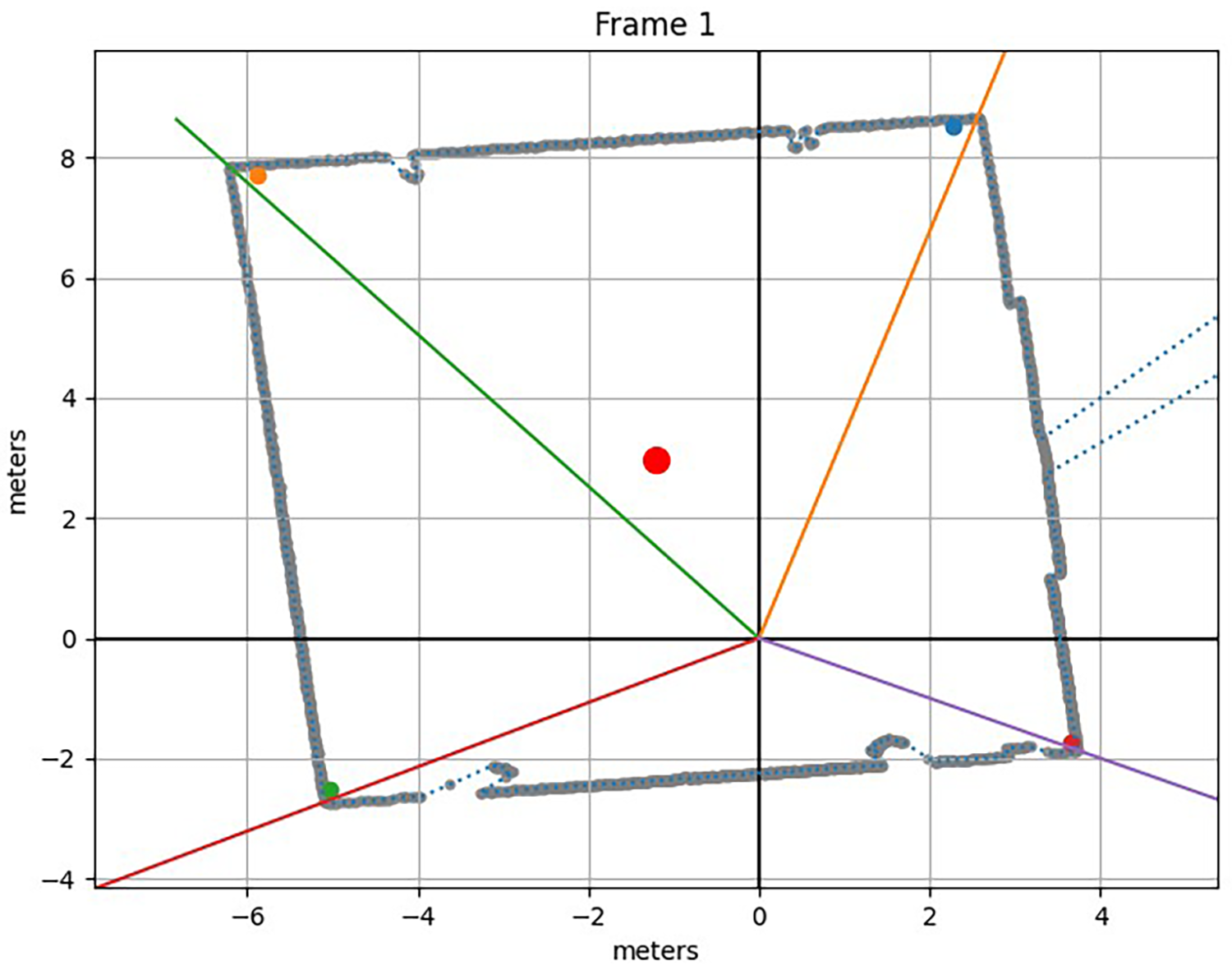
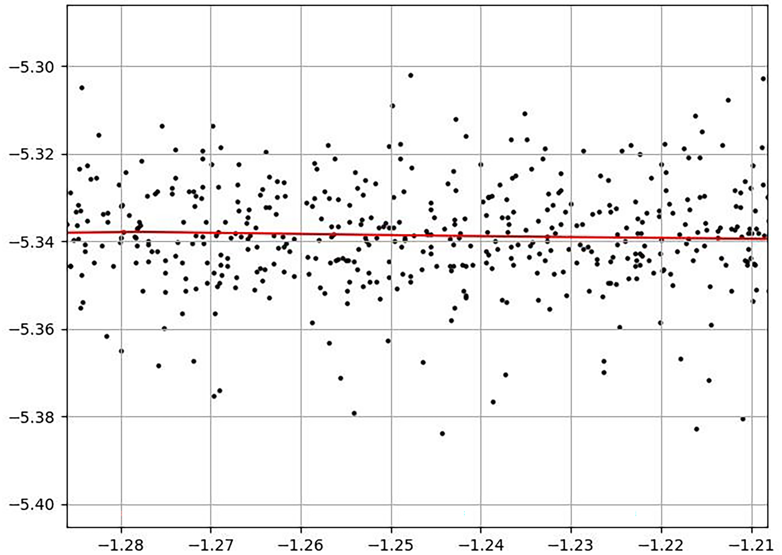
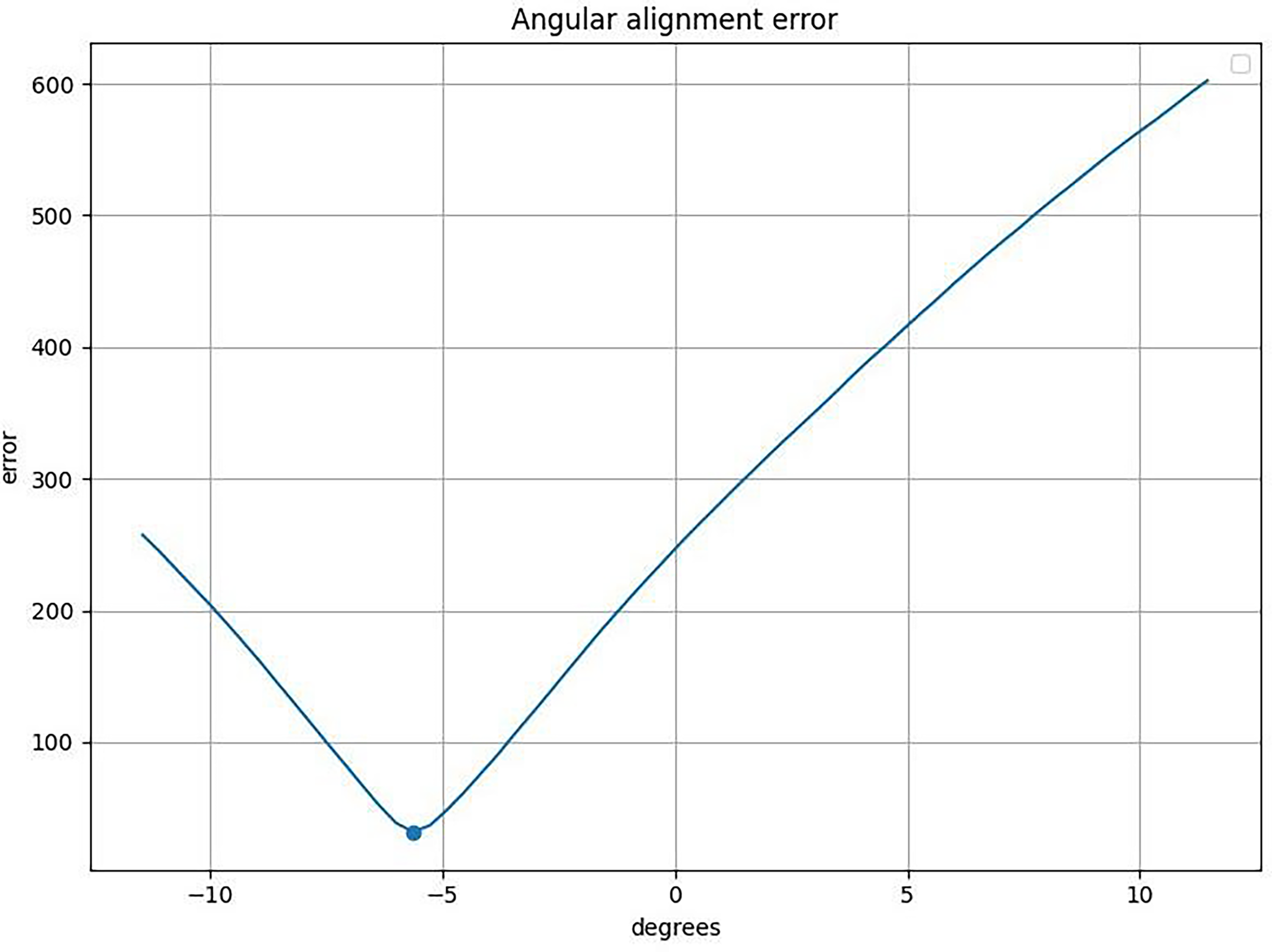
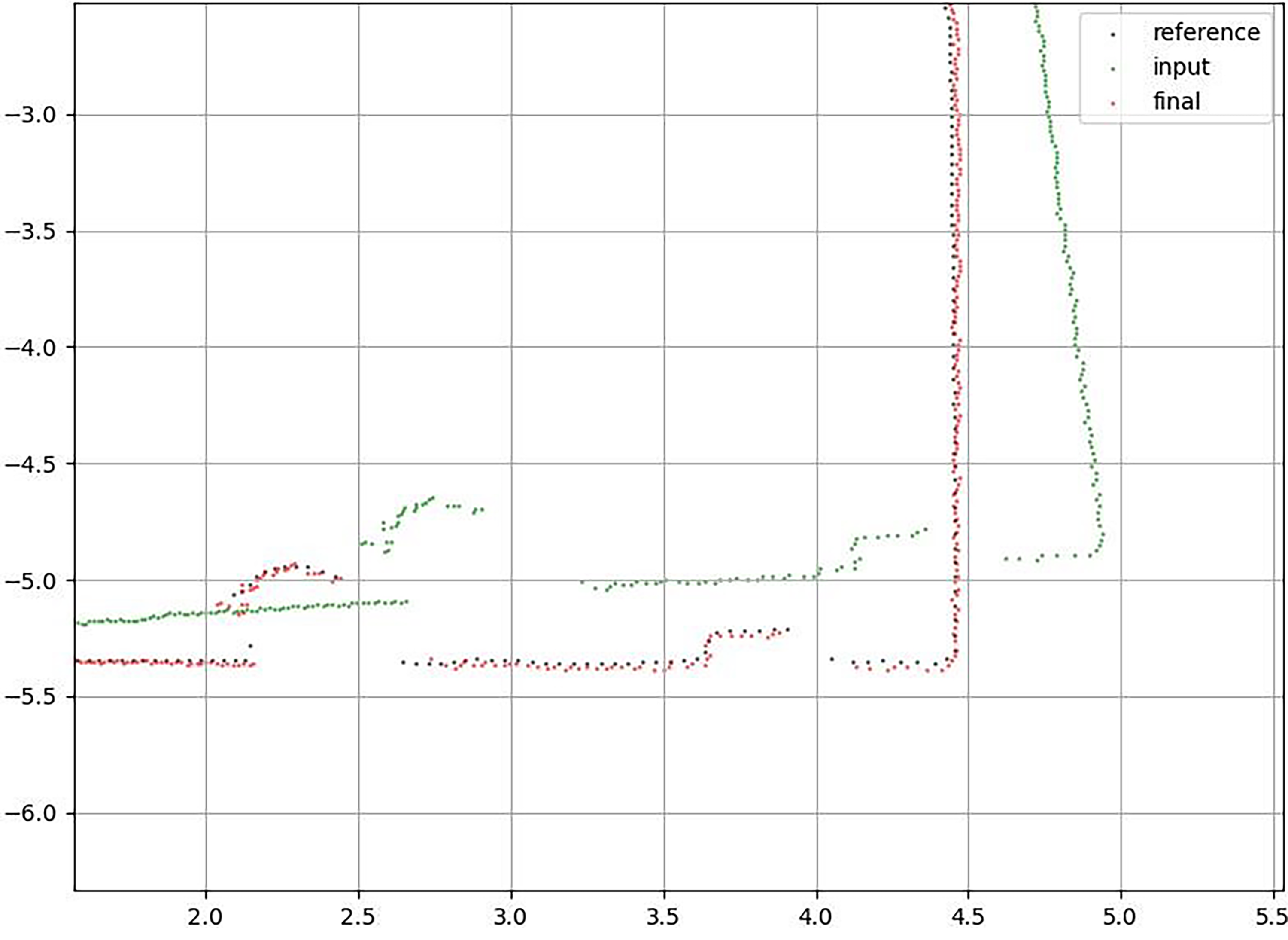
The reference boundary estimate $\hat{B}$ is now used to compute the degree of alignment between the aligned data and the reference boundary $\hat{B}$ . Recall that $\hat{B}$ is the estimate of the ideal measurement in standard orientation. Also, recall that the forklift measures $\vec{r_{k}}$

\vec{r_{k}} = \vec{r} (\vec{s_{k}}, B)

(10)

where the vector denotes the entire angular scan, the subscript k denotes the time or sequence of the measurement, and

\vec{s_{k}}

denotes the unknown pose of the forklift and B denotes the theoretical boundary of the room. If

\vec{σ} \approx \vec{s_{k}}

then using

\hat{B}

, we must have that:

\vec{r} (\vec{σ}, \hat{B}) \approx \vec{r} (\vec{s_{k}}, B) .

(11)

In other words, if the reference room is moved by

\vec{σ} \approx \vec{s_{k}}

and the measurement is simulated using

\hat{B}

, then an approximation of the data can be obtained. Likewise, if the data is transformed by

\vec{σ} \approx \vec{s_{k}}

, then it should approximate the reference room

\hat{B}

. Hence, the best position is defined as the one which minimizes the error function:

\vec{s_{k}} = a r g m i n_{\vec{s}} ‖ \vec{r_{k}} - \vec{r} (\vec{s}) ‖^{2}

The steps are:

Rotational alignment via SGD: first align the forklift by SGD in rotation.

Spatial alignment via SGD: then align the forklift by SGD in space.

Results and discussion

Now, having constructed a reference room, the error between the reference room and any frame and its proposed orientation can be computed. In other words, a given frame can be re-oriented to the reference room and its degree of alignment to the reference room can be computed. This error computation is performed via brute force over a large range of possible positions and orientations and the optimization is also performed via Monte Carlo. The results are then compared.

In Figure 6, the x- and y-axes are in meters. Note the considerable statistical noise between the frames which hinders the pose estimation.

Figure 6.

Superposition of 100 aligned frames showing a corner, a marker, and a room detail.

Refine preliminary pose estimation

It was determined that it is essential to build a reference room to optimize the forklift pose estimation. Figure 6, which shows a detail of the superposition of 100 frames, indicates that there is substantial variation in the location of the landmarks between frames. This will be discussed in a later section. In order to align these frames, an initial alignment was required. The initial alignment uses the previously developed method based upon the neural network. An additional algorithm was developed for refining the corner position obtained from the neural network back onto the raw data. See Figures 7 and 8.

Figure 7.

The refinement of the four corners for a single frame.

Figure 8.

A detail magnification of Figure 7 showing the corner refinement.

The initial corner estimates are shown as dots and the refined corner position via the four colored lines. The x- and y-axes in both Figures 7 and 8 are in meters.

Align against a reference frame

The determination of the corner position allows us to estimate the forklift's pose. Now the measurement of the room can be matched against a reference frame. To achieve this, a reference orientation is defined. In the reference orientation, the room is centered (i.e., the center of the room aligns with the origin of the coordinate system), and the angle of orientation is set at 0 degrees. This means that the markers are at the bottom and the walls are vertical as in Figure 8. This allows to build up a collection of frames to compute the reference room as seen in Figures 9 and 10. In Figure 9, the black dots are the input data, the red dots are the reference data, and the green dots are the output data (i.e., the aligned data).

Figure 9.

Alignment of a single frame to the reference frame in the reference orientation.

Figure 10.

The error function for the frame alignment.

In Figure 10, the left panel shows the error for small shifts of the preliminary alignment to the right and to the left. The color indicates the degree of error (darker color means less error). The center panel plots the central cross sections along x and y to give an idea of the variance of the fit. Note that the error function shows a high confidence of the fit for +/–1 to 2 cm.

Aggregate reference frames to compute a reference room

Many frames are then combined into one dataset. Each of these frames has been aligned with respect to a reference frame and can be an estimate of the true room structure. Thus, a statistical procedure to combine the frames is used to determine the reference room.

In Figure 11, note that there is wide variation for the marker. It seems that at some forklift positions (e.g., near the corner), the marker is not clearly visible to the forklift. The x- and y-axes are in meters.

Figure 11.

A scatter plot of the aligned frames for a marker.

In Figure 12, note the large degree of variation compared to the reference room about the markers. It seems that at some forklift positions (e.g., near the corner), the marker is not clearly visible to the forklift. The x- and y-axes are in meters. In Figure 13, note that 1 standard deviation is about 1 cm.

Figure 12.

A closeup of the reference room (red) along with the data points (black) from which it was computed.

Figure 13.

A closeup of the reference room along with the data points from which it was computed.

Use reference room to align any frame

Once the reference room is acquired, any frame can be aligned to it. This takes several steps: first, the reference room is put in the reference orientation (see previous section); then the frame is put in the reference orientation as best step using the data from previous section. It is then compared to see how much the frame agrees with the reference room. This error computation has some important complications which are not discussed in detail. Intuitively, the minimum distance between the points of one frame and the points of the next frame are computed. The intriguing factor is determining which points should be compared.

Now knowing the forklift orientation in any frame, the room measurement can be transformed into the reference orientation and then compared to the reference room. This is the basic calculation behind the results in the section below.

In Figure 14, the markers are at the bottom and the walls adjacent to the markers are vertical. The x- and y-axes are in meters.

Figure 14.

The reference room in the reference orientation.

Alignment optimization via brute force and Monte Carlo

In principle, the procedure for refining this alignment is simple. In practice, the computation becomes expensive when computed by brute force.

First a spatial increment and a rotational increment must be defined. Then the frame-to-be-aligned must be moved and rotated by these increments, computing the error of the alignment at each one. When the scan is complete, the orientation with the minimal error will be evaluated. This is the “optimal alignment.” While simple in principle, in practice there are several complications. The first is the scale of the optimization. There are three degrees of freedom (two spatial coordinates and one angular coordinate), so the number of orientations that must be explored grows with the 3^rd power of the number of increments. That is, if there are 64 angular and spatial increments, then there are 262,144 orientations to consider. In practice, that is too many to implement in real time. Other issues involve (a) the optimal step size (b) other search conditions that may allow reducing the number of states. Neither issue has been addressed in the present note.

The simplest way to accelerate the search is via Monte Carlo. In simple terms, this means that instead of evaluating every possible orientation, a subset of these orientations is randomly sampled. A variety of probabilistic methods can be used to improve the performance of the algorithm. In the following sections, Stochastic Gradient Descent will be applied to enable mathematical optimization.

In Figure 15, note that the black dots are the reference room, the red dots are the aligned room, and the green dots are the input. The x- and y-axes are in meters.

Figure 15.

Alignment by brute force.

In Figure 16, the rotational alignment of the frames shows the error between the frame and the reference as a function of rotation (from the starting position of the frame). The dot shows discovered minimum at about −5 degrees.

Figure 16.

Rotational alignment of the frames.

In Figure 17, the left panel shows the entire search grid over which the room was shifted in x and in y. The right panel shows the 1D plots through the minimum of the alignment grid. Note the uncertainty is about +/–1 cm.

Figure 17.

Spatial alignment.

Next the brute force is compared to the Monte Carlo method. In the Monte Carlo method, the entire space of possible orientations is not sampled, but instead only a random subset is considered. Figures 18 and 19 show that comparable accuracy is obtained versus the brute force method.

Figure 18.

Alignment by Monte Carlo.

Figure 19.

Spatial alignment.

The black dots in Figure 18 are the reference room, the red dots are the aligned room, and the green dots are the input. Note that the x- and y-axes are in meters and that accuracy is comparable to brute force.

The left panel in Figure 19 shows the Monte Carlo search grid over which the room was shifted in x and in y. The right panel shows the 1D plots through the minimum of the alignment grid. Note that the uncertainty is about +/–1 cm. Also note that accuracy is comparable to brute force.

It has been shown that Monte Carlo performs comparably to the brute force method. It has also been shown that a reference room built from many frames statistically aids in the rapid alignment of frames. A variance of about 3 cm in the accuracy of the pose estimation is seen repeatedly. This range comes up in several contexts: (1) when aggregating the frames for alignment (2) when comparing the reference room to the aggregated frame (3) when comparing any frame to the reference room.

It also seems that forklift velocity impacts the accuracy of the frame. The faster the forklift is moving or spinning, the more that error is introduced into the measurement. This issue has not yet been studied quantitatively. It should certainly be addressed. It is evident that the forklift accelerates during the frame acquisition, causing an apparent bend in a straight wall.

This is not to say that the accuracy is limited to 2–4 cm. However, it is roughly the current accuracy for high confidence: 2 cm when the forklift is stationary and obtains a good measurement, 4 cm when the forklift is moving / accelerating. Note that by 2 cm, it is implied plus or minus 1 cm. And by 4 cm, it is implied plus or minus 2 cm. So, it might be more accurate to report this as plus or minus 1–2 cm accuracy.

Vectoral reference w.r.t center of the room

The next change explored was on the optimization of forklift pose estimation using a vectoral reference. This method is based upon the following facts:

The shape of the room does not change.

If we can determine the (vectorial) location to the center of the room, or any other room landmark, then we can entirely determine the forklift's pose.

From fact 1, a reference room is computed which consists of the entire room, including walls, corners, and reflectors. This room is aligned into what is called standard orientation. It is the room from the perspective of the forklift assuming that the forklift is located at the center of the room with the sensor facing the wall containing the reflectors.

From fact 2, the measurement and the reference room are used to align the forklift. This can be divided into two further steps:

First, simple geometric properties of the room are used to estimate the center. The details are omitted here, but some simple math enables us to roughly estimate the forklift's location and orientation in the room.

Using the reference room, the alignment of the lidar data is optimized to the reference room.

Processing time of algorithms

A major method of assessment would be to check for the time needed to assess the forklift's location. Table 1 shows the time of the computation for each step of the alignment.

The results here show that the spatial align process was sped up by a factor of nearly 400×. Note that these numbers vary since random initial positions were used. Also, note that the larger the uncertainty on the position, the worse that the brute force method will perform, since the number of computations scales with the second power in the size of the uncertainty. The total time for the alignment is about 0.07 s in unoptimized Python.

Comparison of final results

Another major method of assessment would be to check for accuracy of this method against a standard. A sampling of 100 sets of pose data (x, y, θ) were collected and analyzed for both the template matching algorithm and the lidar NAV-350's own software solution based on eight reflectors. At the time of data collection, the orientation angle θ was kept fixed at ten specific predetermined positions. These data sets were then compared against the True Data measured physically in the workspace of 8.9 m by 10.7 m. The average error (Δx, Δy) for the Template Matching algorithm versus the true data is (0.75, 0.79) cm. This number was reduced to (0.62, 0.64) cm when data from close to the walls (within 2 m) were not considered. The average error for the lidar NAV-350's own software was (0.88, 0.89) cm, and this was consistent even when compared against data from close to the walls (within 2 m). The experimental setup was not tested for ranges less than 2 m because the forklift has a base dimension of 1 m × 1.3 m.

The proposed algorithm in this research yields better accuracy when compared against other path planning algorithms using conventional lasers and visual SLAM for indoor tracking. Published research has shown the results of three different SLAM based technologies: SLAMMER, NAVIS and Matterport. The errors reported were 1.7 cm, 3.2 cm, and 4.7 cm, respectively.²⁵

Conclusion

This paper has presented a novel method of localization that was successfully implemented on an industrial sized forklift. The process of taking sensor data from the lidar and applying the necessary mathematics has been described in detail. The results at each step have been discussed in each section of the paper.

The research was performed with one forklift only. Due to budget and logistic reasons, multiple forklifts were not tested. In the presence of any dynamic obstacles, the forklift would need to stop, and the data would have to be acquired at the point where it stopped instead of its initial planned stopping point.

Past research has successfully used SLAM in tracking model robots indoors. The proposed method was also successful in doing the same but using an industry standard forklift. However, it is limited to rooms having corners or angles in the boundaries. Since the markers used were wall corners, any workspace which is circle or oval or devoid of corners would not be applicable to this method.

The results are quite promising as the error is comparable to the industry standard software that uses multiple reflectors to achieve the same level of accuracy. This experiment can be further investigated in the future to attempt better accuracy in results. Use of multiple additional sensors and statistical tools may reduce the error even more. There is also the uncharted area of investigating this concept using multiple forklifts especially in an actual warehouse environment with dynamic obstacles.

Footnotes

Declaration of conflicting interests

The authors declared no potential conflicts of interest with respect to the research, authorship, and/or publication of this article.

Funding

The authors received no financial support for the research, authorship, and/or publication of this article.

ORCID iD

Ebad Zahir

Data availability statement

Data sharing not applicable to this article as no datasets were generated or analyzed during the current study.

References

Truong

Ngo

Nguyen

, et al. A novel infrastructure design of industrial autonomous system. Int J of Fuzzy Logic and Intel Syst 2019; 19: 103–111.

Tran

Ngo

Nguyen

, et al. Implementation of vision-based autonomous mobile platform to control by A* algorithm. In: 2nd International Conference on Recent Advances in Signal Processing, Telecommunications & Computing (SigTelCom), 2018. Epub ahead of print 2018.

Ngo

Nguyen

. Design and implementation of high performance motion controller for 2-D delta robot. Seventh International Conference on Information Science and Technology (ICIST), 2017. Epub ahead of print 2017.

Tamba

Hong

K-S

Tjokronegoro

HA.

Time-varying feedback control of an unmanned autonomous industrial forklift. IFAC Proc 2008; 41: 8582–8587.

Chen

Peng

Wang

, et al. Pallet recognition and localization method for vision guided forklift. In: 8th International Conference on Wireless Communications, Networking and Mobile Computing, 2012; 1–4.

Jeon

Choi

Kim

, et al. Localization of pallets based on passive RFID tags. In: Seventh International Conference on Information Technology: New Generations, 2010. Epub ahead of print 2010. 834–839.

Wang

Liu

, et al. Feature-to-feature based laser scan matching for pallet recognition. In: International Conference on Measuring Technology and Mechatronics Automation, 2010. Epub ahead of print 2010. 260–263.

Fogel

Burkhart

Ren

, et al. Automated tracking of pallets in warehouses: beacon layout and asymmetric ultrasound observation models. In IEEE International Conference on Automation Science and Engineering, 2007, 678–685.

Wang

. Analysis of UWB indoor positioning accuracy based on TW-TOF. Acad J of Sci Technol 2023; 5: 61–64.

10.

Alarifi

Al-Salman

Alsaleh

, et al. Ultra wideband indoor positioning technologies: analysis and recent advances. Sensors 2016; 16: 707.

11.

González

Blanco

Galindo

, et al. Mobile robot localization based on ultra-wide-band ranging: a particle filter approach. Robot Autonomous Syst 2009; 57: 496–507.

12.

Meena

Gupta

Kumar

Analysis of UWB indoor and outdoor channel propagation. In: IEEE International Women in Engineering (WIE) Conference on Electrical and Computer Engineering (WIECON-ECE), 2020. Epub ahead of print 2020.

13.

Zhou

A novel UWB indoor localization algorithm based on TDOA in Los/NLOS environment. In: 4th Information Communication Technologies Conference (ICTC). 2023. Epub ahead of print 2023.

14.

Feng

Guo

Zhang

Q-J

. Recent advances and future trends in Neuro-Tffor Em Optimization. In: IEEE/MTT-S International Microwave Symposium – IMS, 2022. Epub ahead of print 2022.

15.

Zheng

Zeng

, et al. Mobile robot integrated navigation algorithm based on template matching VO/IMU/UWB. IEEE Sens J 2021; 21: 27957–27966.

16.

Harapanahalli

Mahony

Hernandez

, et al. Autonomous navigation of mobile robots in factory environment. Proce Manuf 2019; 38: 1524–1531.

17.

Będkowski

Szklarski

Key Software Components. Autonomous Mobile Mapping Robots, 2023; 1: 33–51.

18.

Thrun

Burgard

Fox

A real-time algorithm for mobile robot mapping with applications to multi-robot and 3D mapping. In: Proceedings 2000 ICRA Millennium Conference IEEE International Conference on Robotics and Automation Symposia Proceedings (Cat No00CH37065); 321–328.

19.

Thrun

. Probabilistic Robotics. Cambridge, MA: The MIT Press, 2005.

20.

Thrun

. Simultaneous Localization and Mapping. Robotics and Cognitive Approaches to Spatial Mapping 2007; 38: 13–41.

21.

Hossen

Zahir

Ata-E-Rabbi

, et al. Developing a mobile automated medical assistant for hospitals in Bangladesh. In: IEEE World AI IoT Congress (AIIoT), 2021, 366–372.

22.

Savage

Contreras

Figueroa

, et al. Construction of roadmaps for mobile robots’ navigation using RGB-D cameras. Intell Autonomous Syst 13: Adv in Intell Syst Comput 2015; 13: 217–229.

23.

Contreras

Mayol-Cuevas

Towards CNN map representation and compression for camera relocalisation. In 2018 IEEE/CVF Conference on Computer Vision and Pattern Recognition Workshops (CVPRW). 2018. Epub ahead of print 2018.

24.

NAV350 Laser Positioning Sensor: Operating instructions. SICK Sensor Intelligence Dec 2022.

25.

Chen

Tang

Jiang

, et al. The accuracy comparison of three simultaneous localization and mapping (slam)-based indoor mapping technologies. Sensors 2018; 18: 3228.

Passive localization of a forklift based on a template matching position tracking algorithm

Abstract

Keywords

Introduction

Conceptual settings

Experimental hardware setup

Mathematical model for localization of the forklift

Mathematical descriptions of parameters used in algorithm

Data analysis: two phases

Phase 1: offline analysis

Phase 2: online analysis

Phase 1: offline analysis

Phase 2: online analysis

Results and discussion

Refine preliminary pose estimation

Align against a reference frame

Aggregate reference frames to compute a reference room

Use reference room to align any frame

Alignment optimization via brute force and Monte Carlo

Vectoral reference w.r.t center of the room

Processing time of algorithms

Comparison of final results

Conclusion

Footnotes

Declaration of conflicting interests

Funding

ORCID iD

Data availability statement

References