Sage Journals: Discover world-class research

Abstract

Reinforcement learning has developed as a promising approach for robot locomotion control, which can save engineering effort compared to conventional approaches. This article presents the implementation of Reinforcement learning on a low-cost, 12 degree of freedom robot known as a quadruped (spider) to optimize locomotion control, enabling the robot to move on different surfaces such as flat surfaces, ramps, speed bumps, and rough terrain. A MATLAB Simulink model is developed as a digital twin of the spider robot. The dynamics of the model were studied and validated using an open-loop algorithm. Then, the model is utilized in a training simulation environment to apply the reinforcement learning algorithm, showing its ability to move along a predefined path as a replacement for conventional motion control systems. Moreover, the work compares the performance and effectiveness of machine learning-based locomotion control with traditional motion control systems regarding navigation accuracy, speed, and adaptability in challenging environments. The minimum hardware requirements are also studied to move the experiment from simulation to reality.

Keywords

Spider robot quadruped reinforcement learning deep learning

Introduction

One of the greatest challenges in rescue missions is the uncertainty of victims’ existence under tons of rubble, where it is hard to measure any vital indicator. Also, the same challenges are found in the maintenance of giant machines or drainpipes where space is limited.¹ Generally, robots are needed to handle complex tasks for humans, and they come in different designs. Robot design mainly depends on the task that the robot will do, the environment where the robot will operate, and the human–robot interaction. Moving from one place to another is the main task of any mobile robot, and the various methods used to accomplish this task are called locomotion. The study of robot locomotion involves understanding how robots navigate and interact with their environment to perform tasks or reach specific destinations. Mobile robots need locomotion mechanisms that enable them to move freely without constraints throughout their environment.² Moreover, locomotion control defines the form or nature of the commands between humans and robots. For example, employing a joystick to control the desired speed and direction is more straightforward for the operator than controlling each actuator’s position (angle) in a four-wheeled robot. But there are a large variety of possible ways to move.

Traditional wheeled robots have significant limitations in terms of locomotion. They have poor obstacle-surmounting ability, poor terrain adaptability, low turning efficiency, or large outer radius, which makes them easy to slip. A legged robot can adapt to almost all kinds of complex terrain, avoid obstacles, and have a wide range of degrees of freedom (DOFs), flexible movement, and even more stability in some cases. With this capability, leg-based robots can be used to rescue humans in all kinds of rocky places, explore all types of complex environments, and potentially perform any physical activity that humans or animals can perform.³

Embedded machine learning (ML) is a rapidly growing field of ML technologies and applications, such as algorithms, hardware, and software, designed to execute sensor data analytics and decision-making directly on devices with minimal power consumption. In robotics, this unleashes the potential of a wide range of applications, and it makes the robot more capable of adapting to environmental changes, using the data, learning from experience, identifying patterns, and optimizing its performance to accomplish a specific task. That applies to all types of robots. For instance, industrial robots powered with ML can be safer, and they are more efficient in obstacle detection, predicting risks, taking real-time decisions to ensure safety, and even predicting their failure. Mobile robots can also be more efficient using ML, optimizing navigation and reducing energy consumption.

As a type of ML, reinforcement learning (RL) has developed as a promising approach for robot learning, which can save engineering effort in conventional approaches. Robots can learn to accomplish tasks by trial and error without previous knowledge of the environment. RL involves discovering optimal actions to take in various situations, aiming to maximize a numerical reward signal. Many RL algorithms have been created to handle continuous action spaces and tested across a diverse set of simulated physics tasks like legged locomotion. There is a growing interest among researchers in applying RL to control robot locomotion instead of conventional control approaches, especially in the case of complex designs such as legged robots, which are considered multi-input, multi-output systems. These robots often present complex systems that demand significant engineering effort for motion control. Yet, the implementation of RL in robotics presents its unique set of challenges. This begins with modeling the environment, which can be a real-world or a simulated model. The first ensures accuracy as the robot interacts with the actual environment, but it comes with risks, as the robot may damage itself while trying to maximize rewards. On the other hand, the second approach enables a quicker learning process where a computing system with higher computation power can be used in training, then the optimal policy can be deployed to the robot hardware. It also minimizes the training cost since there is no risk of damage to the hardware. Still, it may deviate from reality since a gap may exist between the simulation and the real-world scenario. To address this, a well-defined simulation environment that closely mimics reality is essential. Nowadays, many tools and libraries are available for model optimization and to generate C or C++ code to deploy the optimal policy to a microcontroller or small computers.⁴

The rest of this article is organized as follows. The “Literature review” section reviews the literature. The robot design and configurations are discussed in the “Robot design and configuration” section. The dynamic modeling of the spider robot is presented in the “Dynamic modelling of the spider robot” section. The “Reinforcement learning” section discusses the implementation of reinforcement learning. The simulation setup and results are discussed in the “Simulation and results” section. Finally, the article is concluded in the “Conclusion” section.

Literature review

Robot research and design have taken a new trajectory with the advancement of ML. Many researchers are concentrating on empowering robots with the ability to analyze their environment through ML techniques, including object detection and robot tracking,^5,6 debris classification in floor-cleaning robots,⁷ the detection of hazardous materials signs in high-risk operational areas with limited computational resources,⁸ path planning optimization in autonomous guided vehicles,⁹ and several other applications related to visual navigation.¹⁰ In addition, many researchers are developing legged robots to tackle complex locomotion tasks. Achieving agile locomotion in quadruped robots is challenging. Traditional controllers typically require substantial expertise and significant time for debugging and parameter tuning.³ RL offers the potential to address the limitations of conventional controllers by enabling robots to learn effective skills directly from practical trials. This holds great promise in overcoming the constraints posed by conventional controllers. Within this context, considerable efforts have been directed towards quadruped robots, with a more specific focus on mammalian forms of movement, such as dog robots.^11–15 And there has been comparatively less emphasis on applying RL techniques to achieve arachnid-like movement in multi-legged robots. These robots, characterized by the potential for up to eight limbs¹⁶ and the ability to climb and adjust their size, have received less attention in implementing RL-based control strategies. For example, a soft quadruped robot simulation environment was developed by Lagrelius.¹⁷ The robots’ legs consist of a continuum actuator that is driven by three servo motors to achieve complex movements. Each servo motor pulls on a wire attached to the foot of that leg. The work builds upon implementing an RL algorithm based on the MATLAB Simulink environment to train the model’s different walking gaits. Moreover, a bio-inspired hexapod robot called Boogie and its adaptive locomotion controller were presented by Trotta,¹⁸ where an artificial central pattern generator (CPG) was used to generate the robot’s locomotion. It is based on real neurobiological control systems, and it has two layers: The first layer generates typical movement patterns, coordinating the hexapod’s limbs. The second layer ensures adaptability by controlling each limb’s behavior. The adaptability aspect is enabled by an RL algorithm that tunes the parameters of the CPG. The walking behavior simulation was conducted using Simulink Simscape Multibody. In summary, previous works have shown that many real-world problems/applications create different constraints in legged robots’ design, such as size, weight, area, and power. In addition, the complexity of the design plays a significant role in the needed control system, algorithm, and communication hardware. RL-based control strategies show massive potential in controlling legged robots in different environments, but this comes with a price of computational power and how to empower these robots with embedded ML. Moreover, research shows that legged tiny robots are one of the most promising light industries in the world, and they have a diverse range of practical applications that include search and rescue, inspection, entertainment, and STEM education. The learning of tiny-legged robots combines three challenging fields: ML, robotics, and embedded systems.¹⁹

The legged robot designs found in the literature are quadruped and insect robots. Quadrupeds that are found by Fawcett et al.,¹¹ Shi et al.,¹² Li et al.,¹³ Choi et al.,¹⁴ and Lee et al.¹⁵ are inspired by mammals such as dogs and horses. Quadrupeds benefit from a more straightforward gait pattern and the vertical weight distribution over the four legs, enhancing stability and making it easier to control these robots using motion planning algorithms, as found by Silva et al.²⁰ Still, these robots are considered excellent RL applications for controlling locomotion. However, the design of these robots cannot fit in tiny spaces such as tunnels or under rubble, which makes them not the best option for rescue and maintenance operations. In addition, the body cannot adjust its shape according to the environment; most of it weighs > 500 g, disqualifying them as tiny robots. The insect-inspired robot in the literature differs based on the number of legs. The early work on insect robots found by Neubauer²¹ and Shoval et al.²² shows the engineering effort needed to control the locomotion of these robots due to the complexity of the application, and they represent motion planning algorithms for limited situations and robot design. The hexapod presented by Uddin et al.²³ is remote-controlled, requires a communication circuit, and weighs 45 kg. According to Bapat,²⁴ the focus was on the robot design to make it more adaptable to the environment, increasing the complexity of locomotion control. Moreover, the previously discussed works use conventional control approaches that require more engineering effort and cannot generally be implemented in all types of environments. According to Lagrelius¹⁷ and Trotta,¹⁸ a successful implementation of RL to control locomotion on a flat surface is presented. However, hexapods are generally more stable than four-legged robots since the number of legs is higher. Also, they have more DOFs, meaning more actuators, weight, and power consumption. Another insect-inspired design discussed by Wang et al.²⁵ and Oh and Kim²⁶ is spider robots that have four legs and can move in an arachnid way; the work presents different gait algorithms based on the mathematical modeling effort for motion planning without implementing ML.

This study merges the benefits of a simplified quadruped robot design, achieved by using a minimal number of legs to minimize actuator efforts, with the inspiration derived from insects, enhancing the robot’s adaptability in size and locomotion to suit diverse environments. The main challenge is identifying a suitable gait pattern and control strategy to maintain stability during movement since coordinating leg movements, particularly during gait transitions or walking on uneven terrain, needs advanced control algorithms. Therefore, a RL algorithm is implemented to optimize locomotion across various terrains as a replacement for traditional locomotion control approaches.

Robot design and configuration

Robot design

An open-source four-legged robot (spider) design, presented by Swaminathan et al.,²⁷ was built using 3D-printed parts and servo motors. It was controlled using Arduino and a mobile application that communicated via Bluetooth. This work takes the design to new stages: first, the robot is modeled in a MATLAB Simscape for simulation-based testing and evaluation. Second, the robot is trained to walk using RL. The robot is designed with a rectangular body architecture, offering increased area efficiency compared to a circular shape. This design facilitates the straightforward arrangement of essential components such as batteries, controllers, and drivers. The robot’s body is 10 cm in length, 8.5 cm in width, and 2.4 cm in height. The total mass of the robot is < 450 g, including all mechanical and electronic components. Four legs are attached to the corners of the rectangular body, with an assumption that the body’s mass is evenly distributed across these four legs. Moreover, the chosen leg type is inspired by arachnids, selected for its higher stability. Typically, an insect leg comprises six basic parts connected by five different joints. From proximal to distal, they are the coxa, trochanter, femur, tibia, tarsus, and pretarsus.²⁸ Due to its biological complexity, directly mimicking the exact anatomical arrangement of insect limbs would be challenging. Therefore, decreasing the DOFs is necessary to simplify both the mechanisms and control systems.¹⁸

The leg design can be simplified into tibia, femur, and coxa links. The links are connected using three servo motors: body-coxa that rotates around the Z-axis, the coxa-femur joint that rotates around the X-axis, and the femur-tibia joint that rotates around the X-axis. This 3-DOF design guarantees a constant body height above the ground and enables the legs to move in all directions. The final design of the leg is shown in Figure 1. This configuration results in a four-legged robot with 12 joints and four friction contact points on the tip of each tibia, and the contact surface is < 3 mm in diameter. Moreover, the angle of each joint must be limited to avoid unwanted movements and collision between the legs.

Figure 1.

Robot’s leg design.

Figure 2 represents the computer-aided design (CAD) model of the robot. This CAD model is an open source in STL files for 3D printing.

Figure 2.

Four-legged 12 joint robot, computer-aided design (CAD) model.

Inverse kinematics

Kinematics, within the field of mechanics, analyses motion without examining the forces and torques behind it. It focuses on the analysis of position, velocity, and acceleration. Inverse kinematics employs kinematic equations to determine the movement of a robot or its limbs, guiding it toward a specified position. For instance, in the case of a spider leg robot, achieving a specific leg tip position involves calculating the joint angles using inverse kinematics equations. The inputs of the equations are the x and y coordinates of the leg tip and the desired position of the robot body. Therefore, inverse kinematics are utilized in robot modeling to create a logical initial condition that combines the joint’s angles, the desired XY coordinates of each leg, and the desired height of the robot. Also, it is important to randomize the initial states when implementing the RL training to allow exploration. Figure 3 presents the geometric analysis of the front-left robot leg, $θ_{1}$ is the angle of the femur-tibia joint, $θ_{2}$ is the angle of the coxa-femur joint, and $θ_{3}$ is the angle of the body-coxa joint which rotates around the z-axis. The values of the angles $θ_{2}$ and $θ_{3}$ determine the $Z_{o f f s e t}$ , defined as the height between the leg tip and the body-coxa joint. They also determine the value of D, as shown in Figures 3 and 4, which represents the displacement between the leg tip and the body-coxa joint.

Figure 3.

Geometric analysis of spider robot leg.

Figure 4.

Robot top view: Showing the left-front leg fully expanded.

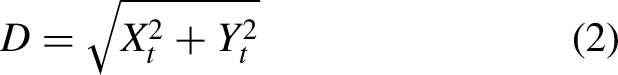
The D displacement can be calculated from the targeted X and Y coordinates of the leg tip about the body-coxa joint, as shown in Figure 4, and the value of $θ_{3}$ determines the ratio between the targeted XY coordinates. When the leg is fully extended $θ_{2} = 0^{\circ}$ and $θ_{1} = - 90^{\circ}$ , D represents the maximum distance that can be reached by the leg tip about the body-coxa joint.

Based on the targeted XY coordinates, the following equations calculate the D displacement and the $θ_{3}$ angle.

θ_{3} = - \tan^{- 1} X_{t} / Y_{t}

(1)

D = \sqrt{X_{t}^{2} + Y_{t}^{2}}

(2)

Another two important values can be obtained from D displacement, which are the R and d displacements, and they are obtained using the following equations:

d = D - C o x a, R = \sqrt{d^{2} + Z_{o f f s e t}^{2}}

(3)

Z_{o f f s e t}

is calculated from the robot body’s desired height (dh) and the offset between the body-coxa joint and the bottom surface of the robot’s body (

B_{o f f s e t}

Z_{o f f s e t} = d h + B_{o f f s e t}

(4)

The

θ_{2}

angle can be calculated by doing the following. First, we calculate the summation of the angles

α_{1}

and

α_{2}

, which are obtained using the law of cosines, and then we subtract the result from

180^{\circ}

to calculate the supplementary angle. Finally, we calculate

θ_{2}

by finding the complementary angle.

\begin{matrix} θ_{2} & = \frac{π}{2} - (\cos^{- 1} \frac{F e m u r^{2} + R^{2} - T i b i a^{2}}{2 \times F e m u r \times R} + \cos^{- 1} \frac{Z_{o f f s e t}}{R}) \end{matrix}

(5)

In the following equation,

θ_{1}

angle can be calculated using the law of cosines and the complementary angle:

θ_{1} = \frac{π}{2} - \cos^{- 1} \frac{F e m u r^{2} + T i b i a^{2} - R^{2}}{2 \times F e m u r \times T i b i a}

(6)

Sensors and actuators

The robot is provided with an inertial measurement unit (IMU) situated at the body’s center of gravity (CG), enabling the measurement of body attitude, velocity, and acceleration. Additionally, each joint has a servomotor capable of producing a maximum torque of 5 Nm. These motors have absolute encoders to measure relative joint angle, joint angle velocity, and the resulting torque. Furthermore, the robot employs force sensors for ground detection, represented as spherical ends and positioned at the tips of each leg. Sensors’ measurements play a crucial role in training deep reinforcement learning. They form the observation vector, which includes all sensor measurements from the robot’s surrounding environment.

Dynamic modeling of the spider robot

A recommended approach in implementing RL involves modeling the environment in a simulation format, reducing computational time, and mitigating the risk of potential damage to the robot hardware during training. Therefore, MATLAB-Simulink is employed in this work to model the spider robot and validate the dynamics of the mode.

Robot design and modeling

The spider model consists of the spider’s body, legs, and the ground, as shown in Figure 5. The inputs of this subsystem are the actions coming from the controller, which is the agent in the case of RL. Moreover, the outputs of this subsystem are the sensors’ readings from the environment. These values are taken from the Simulink-Simscape based on the real-time simulation, and they form the observation vector during the training of the RL agent.

Figure 5.

Spider robot model in Simulink.

The robot’s four legs are linked to its body through the body-coxa joint. This link’s position and orientation are implemented using the frame transformation block based on the CAD design. Each leg contains another two joints: the coxa-femur joint and the femur-tibia joint. The joints are modeled using a revolute joint block acting between two frames with one rotational DOF. The model of the three links in the robot’s leg is shown in Figure 6. The links are connected using the revolute joint block, and the left side of the leg subsystem is connected to the robot’s body.

Figure 6.

Robot’s leg Simulink model showing the frame transformation blocks and the Simscape solid blocks of each link in the leg.

Also, there is an input port for the joints’ torques. The ground contact point of the leg can be found on the right side of the model, and there is an output vector that represents the sensors’ values from the revolute joints, including the angular position and angular speed of each joint. The final robot model can be obtained by replicating the modeling of the remaining three legs using the same approach applied to the initial leg. Variances will exist in the connection points between the legs and the body, determined by the positioning of each leg, the joint’s orientation, and the legs’ components derived from the CAD model.

Design validation

To enable reinforcement learning training for the spider model, it is essential to validate the existing model’s capability to navigate and move in the designated environment. Therefore, a basic movement algorithm has been introduced to coordinate the motion of the four legs, facilitating forward movement along the x-axis. The algorithm contains a series of the x and z coordinates that outline the trajectory of the leg tip for forward motion. These coordinates are translated into joint angles and transmitted to each leg according to its orientation based on the inverse kinematics. Ensuring the forward movement involves transmitting angle values in a timed sequence with a specific delay between the legs. The y-coordinate of the tip is maintained at a constant 60 mm as it does not impact the robot’s movement and restricts the space it occupies during its motion. The desired height can be designated according to the surface, with a minimum value set at 0 mm where the robot touches the floor. For this experiment, it is set at 20 mm.

Forward movement is attained by forward-moving the front-left and rear-right legs along the x-coordinate and altering their positions in the z-coordinate (upward and downward). In contrast, the rear-left and front-right legs move backward in coordination with the other legs. This synchronous movement maintains the robot’s balance, preventing it from falling. Subsequently, the movement pattern reverses: the rear-left and front-right legs move forward in the x-coordinate and adjust their positions in the z-coordinate, while the front-left and rear-right legs move backward only. As a further step in physical model validation, the actual robot model was implemented by printing the CAD model using a 3D printer and assembling the robot parts using 12 servo motors. An Arduino mega is attached to the robot body as a physical model (plant) communicating with the Simulink model and sending the angle commands to the servo motors. The angle values are generated from the trajectory coordinates model shown in Figure 7 and sent to the actual hardware instead of the Simscape model. Figure 8 shows the implemented actual model in Simulink using the servo motor block from Arduino Matlab Support Package.

Figure 7.

Trajectory coordinates model used to validate the design.

Figure 8.

Actual robot subsystem consists of 12 servo motor blocks.

Figure 9 illustrates the resulting movement of the robot, transitioning from point A to point B to represent a single-step movement. The real robot has the same walking behavior as the one resulting from the Simscape simulation.

Figure 9.

The resulting movement of the robot in the Simscape Animation and the actual robot.

Reinforcement learning

Four-legged spider robot locomotion can be formulated as a Markov decision process (MDP) since, at each time step, its state depends only on the previous state at the antecedent time step. At each time step t, the state vector $s_{t} \in S$ describes the state of the agent and the environment at the same time. This vector, rather than a partial observation $o_{t} \in O$ of it, is used by the agent to choose the action for the current time-step: the agent takes the real-valued action $a_{t} \in A \subset R^{N}$ and leads the environment to the very next time step, reaching the new state $s_{t + 1}$ . $S$ is the state space and $A$ is the action space. The advancement to the next time step happens through an environment state-transition distribution $P : S \times A \times S \to [0; 1]$ . $P (s^{'} ∣ s, a)$ is the probability that the environment passes from state s to state $s^{'}$ by means of the action a. Moreover, when a simulation episode begins, the initial state is random $s_{0} \sim ρ (s)$ and each transition process is evaluated by a scalar reward function $R : S \times A \to ℜ$ .^29,30

In RL, an intelligent agent operates in a dynamic environment, aiming to maximize cumulative rewards. The creation of agents contains the development of both the policy and the learning algorithm. In the case of the spider robot, the policy maps 56 observations from the environment to 12 torque actions. The learning algorithm continually updates the policy parameters to achieve the goal, which, in this context, controls locomotion along the x-axis. The agent operates without any pre-existing knowledge of the environment, relying solely on the learning policy for locomotion control. No additional controllers or guidelines are provided to the agent. Figure 10 illustrates the agent’s and the environment’s interaction.

Figure 10.

Reinforcement learning general structure.

The agent is modeled in the Simulink environment using the RL agent block, which serves to simulate and train a reinforcement learning agent within Simulink. This block is connected to an agent stored either in the MATLAB workspace or a data dictionary. The block is configured to receive observations from the modeled environment and a computed reward, also sending actions represented as torques applied to the spider robot actuators. The agent block is also connected to a stopping criterion, which outlines conditions for terminating a training episode in case of poor performance, reducing computational costs associated with undesirable robot behaviors such as falling or losing track. The full model representing the agent and the robot environment is presented in Figure 11.

Figure 11.

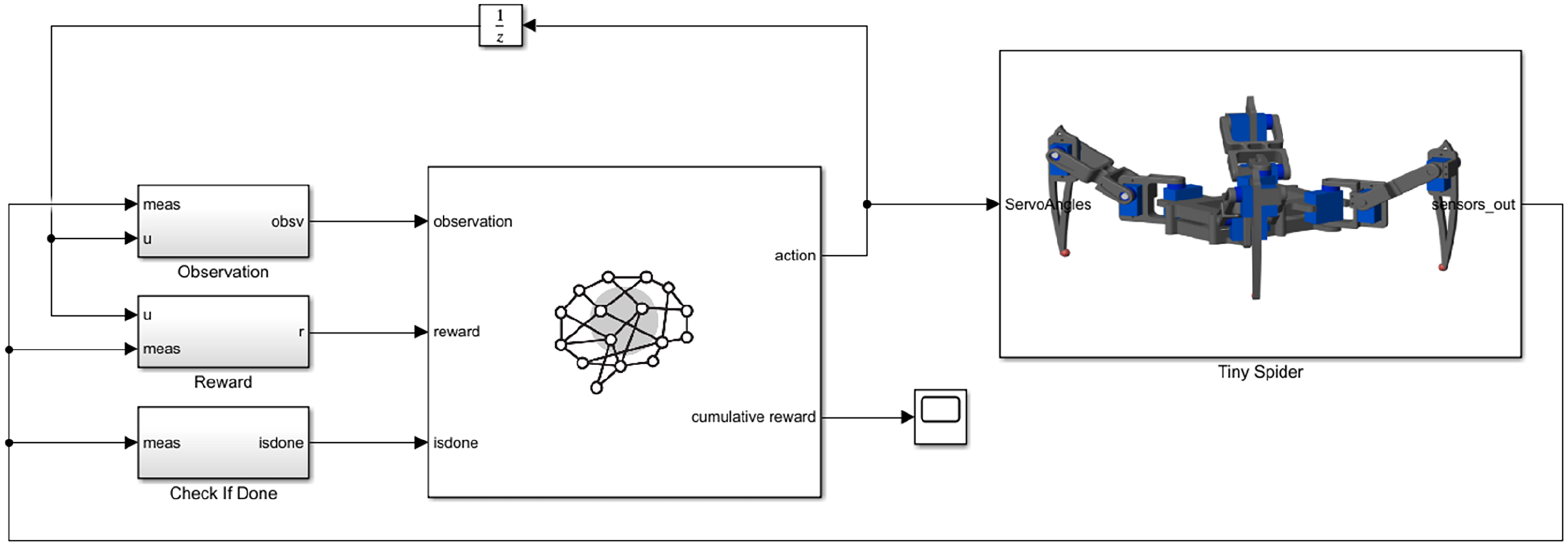
The top layer of the implemented Simulink model.

Choosing the agent learning algorithm depends on the nature of the problem, whether it has a discrete action space or continuous action space. Obviously, the spider robot has a continuous action space where different types of algorithms can be used. In this work, a deep deterministic policy gradient (DDPG) is implemented, showing sufficient results in training the spider agent. However, other options, such as twin delayed DDPG (TD3), can be used and evaluated.

Deep deterministic policy gradient

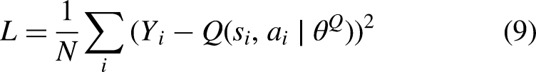
A DDPG is a model-free, off-policy actor-critic algorithm using deep function approximators that can learn policies in high-dimensional, continuous action spaces. It is based on the deterministic policy gradient (DPG) algorithm.³¹ DDPG maintains four neural networks as function approximators: a Q network (critic) $Q (s, a ∣ θ^{Q})$ , a deterministic policy network (actor) $μ (s, a ∣ θ^{μ})$ , a target Q network (target critic) $Q^{'}$ , and a target policy network (target actor) $μ^{'}$ . The target networks are time-delayed versions of the original networks, slowly tracking the learned networks to improve the stability of the optimization. In DDPG, the actor directly maps states to actions instead of outputting a probability distribution across a discrete action space. DDPG also uses a replay buffer. The replay buffer is a finite-sized cache R that stores past experiences. The agent updates the actor and critic using a mini-batch of experiences randomly sampled from the buffer. The implementation of the DDPG algorithm to create an agent of the spider robot can be summarized as follows³¹:

Initialize all the DDPG networks with random parameters and start with an empty experience buffer.

The spider agent takes the current observation and passes it to the actor-network.

The actor-network receives the state $s_{t}$ and generates an action, a small noise value $N$ is added to the action to achieve exploration.

a_{t} = μ (s_{t} ∣ θ^{μ}) + N

(7)

The agent gets a reward $r_{t}$ and a new observation from the environment (next state $s_{t + 1}$ ), the tuple of ( $s_{t}, a_{t}, r_{t}, s_{t + 1}$ ) is stored to the experience buffer R. Then, it samples a random mini-batch of N experiences to learn the policies.

The critic is updated the same as in Q-learning, where the Q value is obtained by the Bellman equation. The value function target is the sum of the experience reward $r_{i}$ and the discounted future reward by a discount factor $γ$ .

Y_{i} = r_{i} + γ Q^{'} (s_{i + 1}, μ^{'} (s_{i + 1} ∣ θ^{μ^{'}}) ∣ θ^{Q^{'}})

(8)

Then the mean squared loss between the updated Q value and the original Q value is minimized to update the critic:

L = \frac{1}{N} \sum_{i} (Y_{i} - Q (s_{i}, a_{i} ∣ θ^{Q}))^{2}

(9)

In the actor, the objective is maximizing the expected return by taking the mean of the sum gradients calculated from the mini-batch N:

\begin{aligned} \begin{matrix} \nabla_{θ μ} J (θ) & \approx \frac{1}{N} \sum_{i} [\nabla_{a} Q (s, a ∣ θ^{Q}) ∣_{s = s_{i}, a = μ (s_{i})} \\ \nabla_{θ μ} μ (s ∣ θ^{μ}) ∣_{s = s_{i}}] \end{matrix} \end{aligned}

(10)

Finally, the agent will update the target actor and critic parameters based on a defined target update method. The DDPG algorithm has significant computational resources requirements. Therefore, in this study, the robot is trained on a well-equipped computer presented in the “Simulation setup” section to minimize the learning time, and only the optimal actor policy, which has less computational requirements and can be handled by an embedded system, will be deployed to the robot to achieve locomotion.

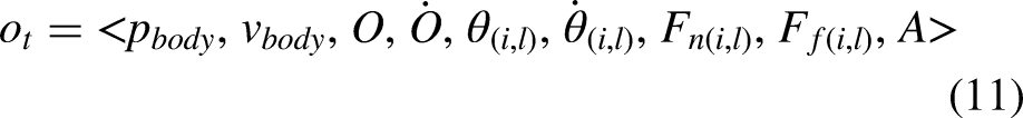
Observation vector

The spider robot interacts with its surrounding environment through receiving observations and executing actions. The actor is responsible for taking actions and learning the task by receiving information from the real robot through an observation vector.

\begin{matrix} o_{t} =< p_{b o d y}, v_{b o d y}, O, \dot{O}, θ_{(i, l)}, {\dot{θ}}_{(i, l)}, F_{n (i, l)}, F_{f (i, l)}, A > \end{matrix}

(11)

where

p_{b o d y}

is the body position,

v_{b o d y}

is the body velocity,

O

and

\dot{O}

are the body angular position and angular velocities, respectively,

θ_{(i, l)}

is the joint

i

position in leg

l

{\dot{θ}}_{(i, l)}

is the joints angular velocity,

F_{n (i, l)}

is the normal force of the contact points,

F_{f (i, l)}

is the friction force of the contact point, and finally,

A

represents the previous actions taken by the agent.

Action vector

The agent generates twelve actions according to the number of the robot’s joints normalized between $- 1$ and 1. After multiplying with a scaling factor via a Simulink gain block, these correspond to the 12 torque signals for the revolute joints. The overall joint torque bounds are $+ / - 5$ N $\cdot$ m for each joint. The action vector $a_{t}$ outputted by the control policy at time t is specified as follows:

\begin{matrix} a_{t} =< u_{i, 1}, u_{i, 2}, u_{i, 3}, u_{i, 4} > \end{matrix}

(12)

Reward function

The agent receives the reward function at every time step during training. Positive rewards incentivize the agent to execute correct actions, while negative penalties discourage it from doing what is wrong. In this work, implementing the RL agent aims to find a locomotion policy that allows the robot to move forward. The reward function motivates the robot to move forward by providing a positive reward for positive forward velocity ( $v_{x}$ ). It also encourages the agent to avoid early termination by providing a constant reward ( $λ_{Δ t} T s / T f$ ) at each time step. The remaining terms in the reward function are penalties that discourage the actor from searching in undesirable states. The term ( $p_{z_{b o d y}} - p_{z_{b o d y, d h}}$ ) is the difference between the instant robot height and the desired height, and it is squared to keep the value positive, this will punch the agent for deviations from the target height. The last term $λ_{u} \sum_{i, l} (u_{t - 1}^{i, l})^{2}$ is the summation of the squared joints torques, and it represents a penalty of using excessive joint torques which will minimize the total actuators effort.

\begin{matrix} r_{t} & = λ_{v_{x}} v_{x} + λ_{Δ t} \frac{T s}{T f} - λ_{z} (p_{z_{b o d y}} - p_{z_{b o d y, d h}})^{2} \\ - λ_{u} \sum_{i, l} (u_{t - 1}^{i, l})^{2} \end{matrix}

(13)

where

λ_{v_{x}}, λ_{Δ t}, λ_{z}

, and

λ_{u}

are positive weights (gains),

p_{z_{b o d y, d h}}

is the desired height of the robot CG along the z-axis. The weight values in the reward function are used to assign relative importance or priority to different components or features of the environment state. The choice of weights depends on the specific task and the desired behavior of the agent. Calculating the weights involves trial and error, starting by initializing the weights to some initial values, then training the agent and evaluating the agent’s behavior to adjust the weights and repeat.

Episode stopping criteria

Episode stopping criteria are essential techniques for implementing the training of the control policy. The training algorithm has the complete freedom to explore the action space, and it could select some actions that could lead to unstable and unwanted states. A logical flag, called the “isdone” flag in the RL agent block, is used when at least one of the modeled stopping criteria is true. The modeled stopping criteria are two: the first one is when the height of the body’s CG from the ground is below a certain $z_{m i n}$ , which means the robot has fallen, the second one is when the roll, pitch or yaw angles are outside bounds, and the robot could have fallen or rolled over. Other approaches are implemented to eliminate unwanted exploration of the states, such as limiting the angles of the 12 joints to avoid physically infeasible movements and control the randomization of initial conditions through the inverse kinematics at the beginning of each episode to provide a balance between exploration and feasibility, enhancing the training process in RL for robotic systems.

Simulation and results

Simulation setup

The training process and the simulation were conducted in MATLAB. Simulink-Simscape is used to model the environment and the RL agent. Deep learning and RL Toolboxes are utilized to create the agent neural networks and perform the RL training. The simulations were performed on a computer equipped with an Intel®Core^TM i9-13900K Processor with 24 cores, a frequency of 3 GHz, and 64 GB RAM. During the training process, RL agents depend on hyperparameters, which are configurations that determine key aspects of the learning process. These parameters control elements like the balance between exploration and exploitation, the discount factor, the learning rate, and the frequency of policy updates. Table 1 shows the hyperparameters that are implemented using the RL toolbox.

Table 1.

Hyperparameter values for the implemented simulation.

Hyperparameter	Value	Hyperparameter	Value
Critic learning rate	$5 \times 10^{- 5}$	Experience buffer length	$1 \times 10^{6}$
Actor learning rate	$5 \times 10^{- 6}$	Discount factor	0.99
Optimizer	Adam	Normalized observations	True
Target update rate	$1 \times 10^{- 3}$	Exploration policy	OU, $θ = 0.15, μ = 0, σ = 0.1$
Batch size	128	Max episodes number	10,000
Iterations per time step	1	Max steps number per episode	400

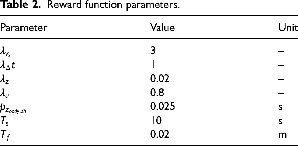
The weight values in the reward function equation (13) are used to assign relative importance or priority to different components or features of the environment state. The choice of weights depends on the specific task and the desired behavior of the agent. Calculating the weights involves trial and error, starting by initializing the weights to some initial values, then training the agent and evaluating the agent’s behavior to adjust the weights and repeat. Table 2 shows the gain values in the reward function subsystem, the simulation time, the sampling time, and the desired height presented in equation (13).

Table 2.

Reward function parameters.

Parameter	Value	Unit
$λ_{v_{x}}$	3	–
$λ_{Δ} t$	1	–
$λ_{z}$	0.02	–
$λ_{u}$	0.8	–
$p_{z_{b o d y, d h}}$	0.025	s
$T_{s}$	10	s
$T_{f}$	0.02	m

Simulation environments

Simulation environments represent different terrains the robot could interact with in real life based on the required application. These scenarios showcase the efficacy of RL training in developing policies for locomotion control across varied terrains. In this work, the agent was trained on five different terrains. The first terrain is a flat surface where the robot must be able to move forward without any change in the surface elevation. The second terrain is called Ramp 1, where the robot must be able to move on a ramp tilted $10^{\circ}$ from the x-axis, and the start position of the robot body is in parallel with the ramp. The third terrain is Ramp 2, where the robot starts moving on a flat surface, then moves over a ramp tilted $11^{\circ}$ for a distance of 1 m, and then walks again on a flat surface. The fourth terrain is Ramp 3, where the robot must overcome a speed bump with a tilting angle of $11^{\circ}$ . The fifth terrain is a rough surface implemented as a surface grid with different elevation values, representing a challenging environment for the robot to walk into. Figure 12 shows the implemented simulation environment.

Figure 12.

The implemented simulation scenarios in reinforcement learning (RL) training.

Simulation results

The training was done separately for each scenario. The training on the flat surface took almost 13 h and reached 8182 episodes. The adopted stopping criteria was an average reward equal to or higher than 50. In the first 2000 episodes, The reward value fluctuates within negative values ranging from $- 90$ to 0, indicating exploration into infeasible solutions within the state space. Then, it stabilizes around 0 with a relatively narrower range of values. After 4000 episodes, the agent discovers a new configuration in the action space, resulting in more satisfactory rewards. The average reward begins to rise until it reaches the training-stopping criteria. To validate the performance, several saved agents were simulated within the robot environment, demonstrating the capability to walk smoothly on a flat surface with an average speed ( $v_{x}$ ) of 0.1 m/s, a value lower than the configured maximum speed ( $v_{x_{m a x}}$ ). Additionally, certain training agents showed sufficient performance, displaying a slight deviation from the y-axis. As shown in Figure 13, The training patterns in Ramp 1, Ramp 2, and Ramp 3 were almost the same as in the flat surface scenario. The training starts exploring the state space, and then it stabilizes around a certain average reward until the agent discovers a new configuration of actions that leads to a higher reward. In performance validation of the trained agents, the saved agents tend to walk cautiously on the different ramps, trying to keep the height of the body on the desired value assigned in the reward function and prevent tilting of the body beyond the limits set for pitch and yaw angles. This cautious approach explains why these agents achieve a lower average reward than the flat surface scenario. The rough terrain is completely different from the previous scenario. The robot’s legs need to adjust to different elevation levels, which change based on the robot’s position on the terrain. However, the agent finished the track with a slight deviation from the y-axis, showing a more conscious walking pace.

Figure 13.

Episode average reward on different types of surfaces.

The optimal actor policy in each scenario controlled the spider robot to move forward along the x-axis, achieving effective locomotion. The agent demonstrated excellent adaptability in adjusting both speed and torque based on the surface. It showed caution by moving slowly on ramps, and unexpectedly, the average torque values on challenging surfaces were lower than on flat surfaces, as shown in Table 3. This unexpected behavior affected the power consumption of the actuators, highlighting the agent’s capability to adapt torque, speed, and power consumption according to the environment.

Table 3.

Average speed, average torque, and cumulative reward.

	Average speed	Average torque	Cumulative
	(m/s)	effort (Nm)	reward $r_{t}$
Flat surface	0.103	4.08	98
Ramp 1	0.071	3.89	67
Ramp 2	0.071	3.9	63
Ramp 3	0.056	3.64	74
Rough terrain	0.062	2.8	59

Simulation to reality

The final step in implementing RL is transitioning from the simulated environment to the actual physical environment, known as deployment. The actor optimal policy can be deployed on the robot hardware to test the optimal policy in controlling locomotion or fine-tune the optimal policy using online learning to get better performance. In MATLAB, a C/C++ code can be generated from the policy evaluation function, which maps the observations to actions based on the developed policy. The generated code can be deployed to the robot hardware, which can be an embedded system and act like a traditional controller. The minimum requirement of such hardware can be specified by analyzing the actor policy using the MATLAB deep neural network analyzer. The number of learnable parameters for the optimal policy model is 146.7k, and since the learnable parameters are stored in a single precision format, taking 32 bits in memory, this neural network has a size of only 0.573 MB.

Conclusion

In this work, a simulation model of a four-legged robot with 12 joints was developed. The dynamics of the model were validated using a basic open-loop algorithm. Subsequently, a RL model employing DDPG was introduced to control the robot’s locomotion. Effectively, the agent exhibited the ability to learn locomotion across various surfaces without the need for conventional control methods nor relying on prior environmental data, showcasing remarkable adaptability and reliability. The training included flat surfaces, ramps, speed bumps, and rough terrains. Moreover, the resulting policies were successfully tested in diverse random scenarios for which the agent had not been trained.

Results and Simulink model availability

The system’s code is public and can be accessed through (https://github.com/ZaidHJaber/Four-legged-Spider-Robot-RL-locomotion). Furthermore, the system demonstration is available. See (https://www.youtube.com/playlist?list=PLrXurzH_oKpuT00fxP0ZjtIjLz9AAMmnC). This transparent sharing aims to expedite model development among fellow researchers and ensure the swift reproduction of results.

Footnotes

Declaration of conflicting interests

The author(s) declared no potential conflicts of interest with respect to the research, authorship, and/or publication of this article.

Funding

The author(s) received no financial support for the research, authorship, and/or publication of this article.

Data availability statement

Data sharing not applicable to this article as no datasets were generated or analyzed during the current study.

ORCID iDs

Zaid Jaber

Belal H Sababha

References

Deepak

Bahubalendruni

Biswal

. Development of in-pipe robots for inspection and cleaning tasks: survey, classification and comparison. Int J of Intell Unmanned Syst 2016; 4: 182–210.

Siegwart

Nourbakhsh

Scaramuzza

. Introduction to autonomous mobile robots. Cambridge, MA: MIT Press, 2011.

Yue

. Learning locomotion for legged robots based on reinforcement learning: a survey. In: 2020 international conference on electrical engineering and control technologies (CEECT). IEEE, 2020, pp.1–7.

MathWorks. Deep network quantizer. [Online]. 2023. Available: https://www.mathworks.com/help/deeplearning/ref/deepnetworkquantizer-app.html.

Kulshreshtha

Chandra

Randhawa

, et al. Oatcr: outdoor autonomous trash-collecting robot design using yolov4-tiny. Electronics 2021; 10: 2292.

Bai

Yang

, et al. Object detection recognition and robot grasping based on machine learning: a survey. IEEE Access 2020; 8: 181 855.

Ramalingam

Lakshmanan

Ilyas

, et al. Cascaded machine-learning technique for debris classification in floor-cleaning robot application. Appl Sci 2018; 8: 2649.

Sharifi

Zibaei

Rezaei

. A deep learning based hazardous materials (hazmat) sign detection robot with restricted computational resources. Mach Learn Appl 2021; 6: 100104.

Chen

Liu

Zhao

, et al. Autonomous port management based agv path planning and optimization via an ensemble reinforcement learning framework. Ocean Coast Manag 2024; 251: 107087.

10.

Chen

Han

, et al. Orientation-aware ship detection via a rotation feature decoupling supported deep learning approach. Eng Appl Artif Intell 2023; 125: 106686.

11.

Fawcett

Pandala

Ames

, et al. Robust stabilization of periodic gaits for quadrupedal locomotion via qp-based virtual constraint controllers. IEEE Control Syst Lett 2021; 6: 1736–1741.

12.

Shi

Zhou

Zeng

, et al. Reinforcement learning with evolutionary trajectory generator: a general approach for quadrupedal locomotion. IEEE Robot Automa Lett 2022; 7: 3085–3092.

13.

Qian

Wang

, et al. Towards generation and transition of diverse gaits for quadrupedal robots based on trajectory optimization and whole-body impedance control. IEEE Robot Automat Lett 2023; 8: 2389–2396.

14.

Choi

Park

, et al. Learning quadrupedal locomotion on deformable terrain. Sci Robot 2023; 8: eade2256.

15.

Lee

Hwangbo

Wellhausen

, et al. Learning quadrupedal locomotion over challenging terrain. Sci Robot 2020; 5: eabc5986.

16.

Álvarez

Rojas

Leon-Rodriguez

. Design and development of a quadruped spider robot. http://robotics.umng.edu.co/publications/2017-UNIBOSQUE-Design%20and, vol. 20, 2018.

17.

Lagrelius

. Comparing four modelling methods for the simulation of a soft quadruped robot. M. Eng. thesis, KTH Royal Institute of Technology, 2022.

18.

Trotta

. Walking motion generation in bio-inspired hexapod robot using reinforcement learning. M. Eng. thesis, The Polytechnic University of Milan, 2021.

19.

Neuman

Plancher

Duisterhof

et al. Tiny robot learning: challenges and directions for machine learning in resource-constrained robots. In: 2022 IEEE 4th international conference on artificial intelligence circuits and systems (AICAS). IEEE, 2022, pp.296–299.

20.

Silva

Barbosa

Castro

. Multi-legged walking robot modelling in matlab/simmechanicstm and its simulation. In: 2013 8th EUROSIM congress on modelling and simulation. IEEE, 2013, pp.226–231.

21.

Neubauer

. A spider-like robot that climbs vertically in ducts or pipes. In: Proceedings of IEEE/RSJ international conference on intelligent robots and systems (IROS’94), vol. 2. IEEE, 1994, pp.1178–1185.

22.

Shoval

Rimon

Shapiro

. Design of a spider-like robot for motion with quasi-static force constraints. In: Proceedings 1999 IEEE international conference on robotics and automation (Cat. No. 99CH36288C), vol. 2. IEEE, 1999, pp.1377–1383.

23.

Uddin

Alamgir

Chakrabarty

, et al. Multitasking spider hexapod robot. In: 2019 IEEE international conference on robotics, automation, artificial-intelligence and internet- of-things (RAAICON). IEEE, 2019, pp.135–140.

24.

Bapat

. Design, prototyping and testing of an autonomous hexapod robot with c shaped compliant legs: Abhishex. PhD dissertation, The University of Texas at San Antonio, 2016.

25.

Wang

Fan

Zhang

, et al. Simulation study of a spider-like robot based on leg reorganization. In: 2021 IEEE international conference on real- time computing and robotics (RCAR). IEEE, 2021, pp.1374–1378.

26.

Kim

J-H

. System design and implementation of multi-legged spider robots for landmine detection in the demilitarized zone. In: 2021 18th international conference on ubiquitous robots (UR). IEEE, 2021, pp.228–234.

27.

Swaminathan

Jaswant

et al. Design and development of light weight and low-cost quadruped robot for spying and surveillance. In: 2022 international conference on innovation and intelligence for informatics, computing, and technologies (3ICT). IEEE, 2022, pp.500–504.

28.

Gullan

Cranston

. The insects: an outline of entomology. Hoboken, NJ: John Wiley & Sons, 2014.

29.

Sutton

Barto

. Reinforcement learning: an introduction. Cambridge, MA: MIT Press, 2018.

30.

Ouyang

Chi

Pang

, et al. Adaptive locomotion control of a hexapod robot via bio-inspired learning. Front Neurorobot 2021; 15: 627157.

31.

Lillicrap

Hunt

Pritzel

, et al. Continuous control with deep reinforcement learning. arXiv preprint arXiv:1509.02971, 2015.