
Abstract
When constructing a multiple automated guided vehicle (multi-AGV) system, it is essential to calculate the potential values of the system’s feature parameters. This article presents two time-cost calculators and an improved simulation platform for scientifically estimating the cost of constructing a multi-AGV system. By inputting the parameters of the number of automated guided vehicles (AGVs), the velocity of the AGV, the number of tasks, scheduling interval and path length, the designed calculator can output the system’s time expense when all tasks are completed. The designed simulation platform can display a specific multi-AGV system’s time cost and how the entire progress works in a visual interface. An advanced scheduling method based on handover mode and A* algorithm is used to solve task scheduling problems in a multi-AGV system. The overall performance of the newly integrated scheduling system is compared with other scheduling systems to validate its superiority and shortcomings in different corresponding work scenarios. The final results present a robust solution to improve a multi-AGV system’s effectiveness.
Introduction
Robots equipped with a series of sensors have been widely used in industrial areas. Multi-AGV systems are the most commonly used multi-robot system in different scenes. However, how many AGVs should be used in certain scenes to make the system have the highest efficiency and what method should be used to make the system have the highest efficiency are challenges to establishing a multi-AGV system.
There are many precedents for scheduling optimization methods, but most of the solutions are for the independent tasks of a single AGV, and little attention has been paid to the mutual assistance problem in AGV cluster scheduling. For example, when vehicles cooperate with each other to realize the mutual transfer of goods and other operations. If the cooperation of AGVs is not considered, although some methods and the actual movement path and task allocation of each AGV are optimized as much as possible, the empty AGVs that have completed the task will become invalid resources and occupy space and time in the whole system. Improvements to AGV scheduling systems have become a focus of research. In terms of the overall architecture of the AGV scheduling system, Zając and Małopolski proposed in 2021 to divide the traffic network into nonoverlapping regions and to analyze it as a discrete event system. 1 In other words, this approach allows the system to consider the global problem by successively solving local problems. In contrast, De Ryck et al. argue that most current systems that work centrally lack flexibility, robustness, and scalability. 2 There is an increasing amount of research proposing the decentralization of AGV systems, and decentralized systems should be the future trend. However, the fact is that no authoritative company or research team has yet succeeded in developing a set of standards that are generally accepted by the market or the academic community. How to establish a scheduling system architecture that can be adapted to any practical situation in the relevant field should be a topic that needs to be explored for a long time.
According to the existing literature search, when solving the problem of maximizing the effectiveness of multi-robot cluster scheduling, the research on path planning, obstacle avoidance algorithms, and scheduling mechanisms rarely consider the handover rule, and after the addition of the handover rule, the optimization and combination of path planning, obstacle avoidance algorithms, and scheduling mechanisms require to be added with other considerations when facing specific scenarios. Therefore, this article adds the consideration of handover rule to construct the calculator, simulation platform, and optimization of scheduling method. The A* algorithm possesses optimality, rapidity, and extensive applicability. Under certain conditions, the A* algorithm is guaranteed to discover the shortest route. Compared to other search algorithms, the A* algorithm is faster because it is able to reduce the number of paths to be searched via heuristic functions. This makes the algorithm very efficient when dealing with large-scale search problems. Furthermore, the A* algorithm can be applied to solve a variety of path search problems, such as finding the best path in a computer game and finding the shortest path in robot navigation. The A* method is adopted because of its classical nature, and by comparing it with other algorithms, we consider that the simulation platform and scheduling method built with the A* algorithm and the handover rule can serve as a good foundation for future optimization and innovation.
Based on the typical working progress for the multi-AGV systems, a special calculator is created. It has two modes: basic mode and handover mode. It can calculate the time for the system to complete all tasks based on the input parameters. Furthermore, three working models are raised to test the cost of the multi-AGV systems. A simulation environment is created. The simulation can specify the number of workstations of the current scheduling system, the number of AGVs, and the shortest path algorithm. There is a timer that will run when the simulation starts. The system adds a new task target to the task list according to the exponential function cycle. When the task is released, the scheduling system assigns an idle AGV to receive it. It needs to load the goods to the first station in the task and then drive to the second station to unload the goods. The second station needs time to process the unloaded goods, and the unloaded AGV waits for the reallocation of the scheduling system. By using different scheduling optimization methods, it can be concluded which scheduling optimization method has the best performance.
In summary, our major contributions are as follows: We generalize a special calculator to compare the time cost of the basic AGV system with the time cost of the AGV system using handover mode. We propose an improved simulation platform based on the A* algorithm and apply it to a specific AGV system’s simulation. We present a solid theoretical analysis for our simulations and test the solution by experiments with randomly generated data.
This article’s remaining sections are organized as follows: The second section presents other papers related to this work. The third section shows details of our approach. Experimental results are discussed in the fourth section before the conclusion in the fifth section.
Related work
The AGV systems are an attractive solution for increasing the level of automation in factory areas. The environment an AGV system works in can be divided into a static environment and a dynamic environment. Each environment can also be divided into unknown environment, known environment, and known environment with established paths. For AGVs, the research is focused on improving individual AGVs’ function 3 –7 or multi-AGVs’ scheduling methods. 8 –12 The main environment in industrial applications is a known environment with established paths.
There are two main research directions in a multi-AGV system established in a known environment with established paths. One research direction is the dispatching strategy. The other research direction is algorithms that contain path planning algorithms and obstacle avoidance algorithms.
The AGV dispatching strategy is to solve the problem of assigning loads to vehicles or vehicles to load when they are available. Kızıl’s team raised a dispatching rule that maintains the system operational at all times. 13 Currently, the AGV dispatching strategy could be one AGV chosen to respond to work center’s service when only one work center applies service and other AGVs are free. The AGV dispatching strategy could also be a work center serviced by AGV when only one AGV and more work centers apply service at one time. 14 Egbelu’s team solved the work center-initiated task assignment dispatching problems and vehicle-initiated task assignment dispatching problems. 15 Egbelu presented an algorithm that assigns load movement priority based on the demand states of the load destinations. 16 Co’s team outlined the vehicle management control strategies discussed in previous studies on AGVs in 1991. 17 Pyung-Hoi’s team presented a vehicle dispatching procedure based on the concept of the theory of constraints, in which vehicle dispatching decisions are made to utilize the bottleneck machines at the maximum level. 18 Marvizadeh and Choobineh presented the algorithm with the objective of load balancing among the factory work centers by choosing the dispatch decision, which contributes the most to the laminar flow of the factory. 19
From an algorithmic perspective, scheduling optimization of multi-AGV systems broadly consists of three areas, namely task allocation, path planning, and collision avoidance. There are many precedents for research in these three areas. For task allocation, Yuan et al. 20 studied the dual-resource integrated scheduling problem of AGVs and machines in an intelligent manufacturing shop floor environment, taking into account the constraints of machines, workpieces, and AGVs. Mengyuan et al. 21 and De Ryck et al. 22 proposed a decentralized solution to achieve flexible and self-organized AGV task allocation. Li et al. 23 developed a multi-objective mathematical model for AGV scheduling. Bao designed an auction-based heuristic 24 and experimentally verified that a hybrid allocation rule for AGV and tasks can also be a better choice, as opposed to sequential allocation. In his latest research in 2022, Fazal et al. proposed a task allocation technique based on threshold levels. 25 Its use of the threshold level as a reference for task acceptance, the scheme has led to a significant improvement in the resource utilization of the system.
For path planning, Lian et al. proposed an improved heuristic path planning algorithm that converts energy consumption into the overhead of the path planner. 26 Majdi et al. 27 used fuzzy control techniques to navigate multi-AGVs in an unknown environment. Yu et al. developed a mixed integer planning model for multi-AGV systems in path planning, 28 which has the advantage that it can be transformed into a series of subproblems before solving them one by one under certain conditions and adds penalty terms to the algorithm for generating paths. Digani et al. 9 proposed an integrated approach based on a two-layer control architecture and automatic algorithms, as well as some classical algorithms such as A* Algorithm, Dijkstra Algorithm, and Ant Colony Algorithm. 29 –31
Breadth-first search (BFS) is a traversal strategy for connected graphs. The idea is to start at a vertex and radially traverse a wider area around it preferentially. 32 Depth-first search (DFS) is a search idea, compared to the BFS, DFS for each branching path to the depth of the depth cannot be deeper. It can be applied to the traversal of the tree/graph, nested relationship processing, backtracking, and so on. 33 Best-first searching is a heuristic search algorithm, which can be viewed as an improvement of the BFS algorithm. It uses a heuristic valuation function to value the points that will be traversed and then selects the less expensive ones to traverse until the target node is found or all points are traversed and the algorithm ends. It does not guarantee that the path found is a shortest path, but the computation process is much faster compared to Dijkstra’s algorithm. 34 IDA* is an A* algorithm that employs an iterative deepening algorithm. Since IDA* has changed to a depth-first approach, it does not require weighting or sorting compared to the A* algorithm, which is favorable for deep pruning. It reduces space requirements and is actually a DFS at each depth, although the depth is limited. However, the difference between the two searches before and after is tiny, and every time the depth changes in the backtracking process, we have to search from the beginning again. 35 D* Lite is to identify and process those points that really affect the final path and try to ignore the computation of irrelevant points, so as to improve the computational efficiency when pathfinding again. 36 The above-mentioned algorithms and their characteristics are summarized in Table 1.
Scheduling algorithms.

BFS: breadth-first search; DFS: deep-first search LPA*: Lifelong Planning A*; IDA*: Iterative Deepening A*.
For collision avoidance, it is usually considered together with the design of the path algorithm. The basic idea is to avoid or give way in advance, for example, Liyun et al. designed collision avoidance factors to guide AGV to avoid collisions. 37 However, due to the AGV’s own limited sensors and actuators, there are many unexpected contingencies in practice. To address this direction, Luo et al. proposed a design method for a maximum permissible (optimal) controller based on Petri nets (PNs), 38 using tags to label indistinguishable events. In this way, with the help of the PN model, the collision-free problem is formalized as a combination of linear constraints, significantly reducing the computational overhead due to uncontrollable events.
Furthermore, robot simulation platforms typically have the following capabilities: rapid robot prototyping, motion simulation utilizing a physics engine, and control of simulated or actual robots via scripting programs or network communication. USARSim is a simulation platform for designing high-fidelity multi-robot environments based on the Virtual Arena Engine. Mainly for ground robots, it employs the Open Dynamics Engine (ODE) supports 3D rendering and physical simulation, higher configurability and scalability, compatible with Player, using a layered control system, open interface structure simulation functions, and tool framework modules. 39,40 Simbad is a Java3D-based multi-robot simulation platform for research and educational purposes. It primarily focuses on some simple basic problems of artificial intelligence, machine learning, and more general AI algorithms in multi-robot systems that users are passionate about. It has features such as programmable robot controllers, customizable environments, and custom configurable sensor modules, uses 3D virtual sensing technology, supports single or multi-robot simulation, and supplies toolboxes such as neural networks and evolutionary algorithms. 41,42 Webots is a mobile robot development platform with modeling, programming, and simulation, mainly for ground robot simulation. Users can design a variety of complicated heterogeneous robots in a shared environment with customizable environment sizes, and the characteristics of all objects in the environment, including shape, color, text, quality, and functionality, can also be freely configured by the user. It uses ODEs to detect object collisions and simulate the dynamics of rigid structures and can accurately simulate physical attributes such as object velocity, inertia, and friction. 43,44 The calculator and simulation platform proposed in this article focuses on simplicity, efficiency, and great scalability. Users can efficiently calculate the expense required to construct a multi-AGV system without overly complicated settings and at the same time can efficiently optimize and integrate the path planning algorithm, obstacle avoidance algorithm, and scheduling mechanism.
In summary, comparison with other simulation platforms, the designed multi-AGV systems’ scheduling optimization method is a method that includes an AGV dispatching strategy, path planning algorithm, obstacle avoidance algorithm, and scheduling rules to optimize the whole multi-AGV system. Our focus is on finding a way to improve a specific multi-AGV system’s performance in a known environment with established paths.
Scheduling optimization method
A special calculator that contains two modes, basic mode and handover mode, is created to compare the time cost of the basic AGV system with the time cost of the AGV system using handover mode. After that, a simulation platform is established based on the A* algorithm and applied in a specific AGV system’s simulation to discuss the feasibility and actual effect of cargo transfer between multiple AGVs and judge the differences and optimization points between different scheduling systems.
Time-cost calculator
Two time-cost calculators are created. One is called a one-path time-cost calculator. The other is called the N-path time-cost calculator. The structure of the one-path time-cost calculator can be seen in Figure 1. First, a series of parameters are input in the calculator, which contains the number of AGVs


The one-path time-cost calculator’s structure.
In this function, t is the running time of the system, di is the length of one path, and v is the velocity of the AGV. The handover mode means there is no limit number of AGVs on one path. If two AGVs collide, one AGV will hand over the task to the other AGV and change direction. If no task needs to be dispatched, it will not send a new AGV. If all the tasks are completed, all AGVs will return to their origin. If the system can dispatch AGV continually, there will be a formula
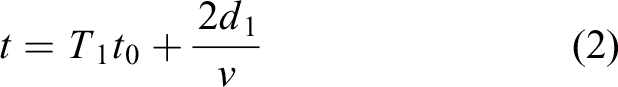
In this function, t is the system time, t 0 is the scheduling interval, T 1 is the task number, d 1 is the length of the path, and v is the velocity of the AGVs. Due to the continuity of distribution of the system, the first term on the right of the equation gives the moment of the last AGV dispatched. The second term is the time AGV needed to run forth and back. Adding both terms together can get the total system running time.
In the handover mode, as long as all tasks are not successfully delivered, it will call itself circularly until all tasks reach the target point. The algorithm will successively calculate three types of event nodes before all tasks are completed, which are regular collision node, boundary collision node, and scheduling interval node. Regular collision node means the collision between two AGVs in the path. In the handover mode, the conventional collision is the handover of tasks. The front AGV needs to hand over the tasks to the rear AGV. After the handover, the two AGVs run in the opposite directions, respectively. The boundary collision node means that an AGV has successfully delivered the mission or returned to the origin. The successfully delivered AGV returns directly, and the AGV returning to the origin will be added to the queue waiting for dispatch. The scheduling interval node means that when the scheduling interval reaches the T value, new tasks can be sent to AGV for transportation.
In the handover mode, the program needs to find the latest event node. Therefore, the program needs to judge which of the three event nodes is closest to the current time. If the nearest event node is found, the calculator will update the status of the AGV participating in the event according to the definition of the corresponding event node and update the location of other AGVs in the path. After the update, the calculator will add the time difference between the node time and the current time to the total system time.
When all tasks are successfully delivered, the calculator will stop calling method handover. At this time, it is no longer necessary to let the AGV handover, so all AGVs need to return to the origin. The calculator will finally calculate the time of this period and add it to the total system time. When all AGVs return to the origin, the total time of the output system will be showed.
The structure of the N-path time-cost calculator can be seen in Figure 2. First, the input parameters are the same as the one-path time-cost calculator’s input parameters. The number of the path and each path’s length should also be input. Because there are N paths, the program will call the handover method N times. When the handover method is called, a back object is defined to store the AGV information on the path. Unlike the three event nodes of the one-path algorithm, which are the conventional collision node, the boundary collision node, and the scheduling interval node, the N-path algorithm needs to consider the AGV return on the past path to schedule the AGV for the new path. Therefore, it needs an additional event node, that is, the return event node. Then, the method will calculate a series of event nodes on this path in turn. Each event node corresponds to a period time t 0. Because we need to consider the situation of the past paths, we need to call the time_handover method on other paths within t 0 to update the AGV information on the past paths. In the time_handover method, it needs to receive the sequence number and period time t 0 of the parameter path and update the AGV’s information within this period time. Because the task has been dispatched, there is no need to consider the scheduling interval node. Therefore, only the regular collision node and the boundary collision node are necessary. The calculation principle is the same as the one-path. When the task dispatched by each route meets the requirements, it will exit the loop and store the back object in the dynamic array to update the path information. After that, the program will continue to call the handover method until n times. After calling n times, the program will wait for all AGVs to complete the task. When all the tasks arrive at the destination, there are no tasks on the path at this time. Therefore, the handover mode stops at this time, and the program will make all AGVs return to the destination. Finally, when all AGVs return, the N-path time-cost calculator records the time and outputs the system’s total running time.

The N-path time-cost calculator’s structure.
In case of handover time is zero seconds, the scheduling priority principle shall be met in any case. That is, the longer the path, the greater the scheduling priority, to meet the minimum running time of the system. When the scheduling system can send AGV continually, there is a mathematical formula to calculate the system time

In this special case, it is easy to get what is the final AGV to come back to the origin. In this formula, each term means the last moment of an AGV comes back to the origin. Ti
is the number of tasks of each path, di
is the length of each path, t
0 is the scheduling interval, v is the velocity of AGVs, and t is the system time. The goal is to find out the moment each path’s AGV which is the last one comes back to the origin. Due to the continuity of the dispatching, as for the path of index i, the last dispatching moment is
In summary, the designed calculator builds a mathematical model based on conditions such as the size of the factory, the number of AGVs, and the number of shelves in the factory in the AGV usage scenario. The calculator designed based on this model can derive the time consumed by different AGV clusters to complete all tasks in different work scenarios. The designed calculator is highly scalable and the A* algorithm was used in this test to verify the effectiveness of the designed calculator. In the future, we will develop a calculator based on the current calculator with a visualized interface, more input parameters, and the ability to easily import path planning algorithms, obstacle avoidance algorithms, and scheduling mechanisms designed by the researchers themselves, which will help the researchers or the enterprises to compare the different combinations of path planning algorithms, obstacle avoidance algorithms, and scheduling mechanisms in building the AGV scenarios of their needs and to provide scientific data support to reduce cost and improve efficiency.
Simulation platform
The simulation platform is established based on Lin and Hsyu’s design. 25 As shown in Figure 3, the meaning of the parameters in the figure is as follows:
Center (class): It is used to initialize a scheduling system. It contains several parameters that are the number of AGVs, the number of workstations, the AGV navigation algorithm, parameters that can define the used path rules, and so on.
Process(navigation()): All moving parts, such as AGVs, can be simulated with Process. Therefore, a separate process, Process(navigation()), is used here to schedule the work arrangement of each AGV.
VehicleID(): It is a method of assigning new tasks to AGV. It will schedule a new task path arrangement for AGV. It includes the current path to be executed, vehicle.path and the path to be executed in the next stage, vehicle.nextpath.
Job_arrive(Periodic entry): This method will randomly generate a task type and add it to the task list of the scheduling system. Meanwhile, this is a periodic method that will be called repeatedly after a certain time interval.
Create(Jtype): This method is built into the Job_arrive. When the Job_arrive is called, a new task type will be generated through this built-in method. Similarly, using independent progress to call flow() to record the completion status of the task type and call WorkstationID() in time.
WorkstationID(): This method will be called after the workstation completes the processing task and will require the scheduling system to assign one or two AGVs to load the finished goods.

The simulation platform’s structure.
When the simulation platform starts, the user can specify the number of workstations in the current scheduling system, the number of AGVs, and the algorithm for picking the shortest path when the AGVs are running. After the timer has been set, the system begins a periodic cycle of adding new task targets to the task list. To mimic as closely as possible the daily work scenario of a production plant, the tasks are designed in such a way that they contain in turn all the workstations that need to handle the goods. When the task is first posted, the scheduling system assigns an idle AGV to pick it up. It needs to load the goods at the first station in the task and then travel to the second station to unload the goods. At this point, the second station needs time to process the unloaded goods, while the completed AGV awaits reassignment from the scheduling system. After a period of processing, that station updates the current status of the task and reissues it to the task list. Then the scheduling system assigns an idle AGV to pick up the task again and, depending on the current status of the task, loads the goods from the second station and goes to the third station to unload them. This is done until all the requirements of the task have been completed.
When the AGV performs the movement operation in the system, it is necessary to mark each step of the AGV’s movement. It means when the AGV performs the movement operation, it first needs to make an arrival application for the intersection of the table path in the scene. The reachable intersections in the scene can be described by a concise two-dimensional list I

In function 1, x refers to the horizontal axis coordinate point of the two-dimensional list, and y refers to the vertical axis coordinate point of the two-dimensional list. Therefore, every time the AGV moves to the next intersection in the scene, it can add a request instruction for its next target point, so that other vehicles can judge its next action arrangement.
When the scheduling system schedules the operation of AGV according to the task list, the current movement request has the necessary target point and starting point. Meanwhile, the current AGV will start to perform transportation operations. A mobile request T can be described with concise symbols

p(T) is all the reachable intersection points in the scene, except the points blocked by the workstation. d(T) is the delivery point of all workstations including the warehouse and charging station.
Each newly created task is a new process instance, that is, the process will continue to loop until the task is completed. Each time it is updated, the scheduling system looks for a new idle vehicle by means of the workstationID function. In addition to this, each AGV has its process instance, which calls the VehicleID function in a loop, to ensure that the AGV’s movement path is updated and to avoid vehicle conflicts when they occur.
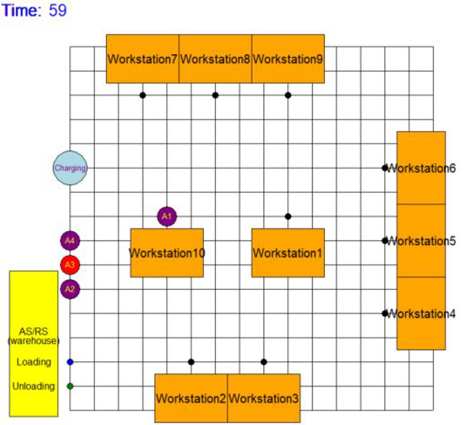
The scheduling system for this project is shown in Figure 4. The blue time label in the upper left corner records the current simulation time in the event-based simulation execution environment, where the passage of time is simulated by stepping in from one event to another. The 6 AGV machines are represented by purple marked points such as A1 and A2, and the 10 distribution points (represented by orange rectangles Workstation1, Workstation2, etc.) in the two-dimensional plane are used for parcel scheduling distribution. Considering the power loss of the AGVs, a blue charging station is set up to realize the energy replenishment of the AGVs. It is also the idle waiting point and starting point for the AGVs. In addition to this, the lower left corner of the system contains a yellow rectangle of the main goods storage room, with a blue dot and a green dot representing the loading and unloading points of the storage room, respectively.
Live demonstration.
The tasks to be handled are randomly added to the task system with the target workstations that need to be visited in turn. Under the overall assignment of the scheduling system, the idle AGV picks up the task and starts the handling work. When the AGV is carrying a load, its color changes to red. The vehicle will enter the charging station in two situations: Once the vehicle’s charge level has fallen below a certain level. When the AGV is idle after unloading the goods and there is no demand for new task scheduling at the moment. The vehicles travel on a grid-like network-guided path, with the vehicles traveling in the following directions: up, down, left, and right. The scheduling system then continuously cycles through the release of tasks and simultaneously modifies the task status of each AGV before the cut-off time, dynamically adjusting the scheduling arrangements as a whole. This enables the individual AGVs to continuously maintain optimal working conditions until they reach their minimum power level, maximizing the overall scheduling efficiency of the system.
Figure 5 shows how the simulation platform works. The simulation platform builds a scenario for AGV operation by setting the number of nodes and edges, which includes workstations, charging points, and warehouses. The scenario contains workstations, charging points, and warehouses. After building the scenario, the platform will count the values of the defined parameters, including path length, number of AGVs, number of tasks, task content, and speed of AGVs. After that, the platform will run the selected path planning and scheduling methods, and in the future, it is planned to improve the scalability so that users can import the methods from outside into the platform. When all of the above is complete, the platform will display the flow of the entire AGV system operation on the graphics user interface (GUI) and output the results of the completed tasks.
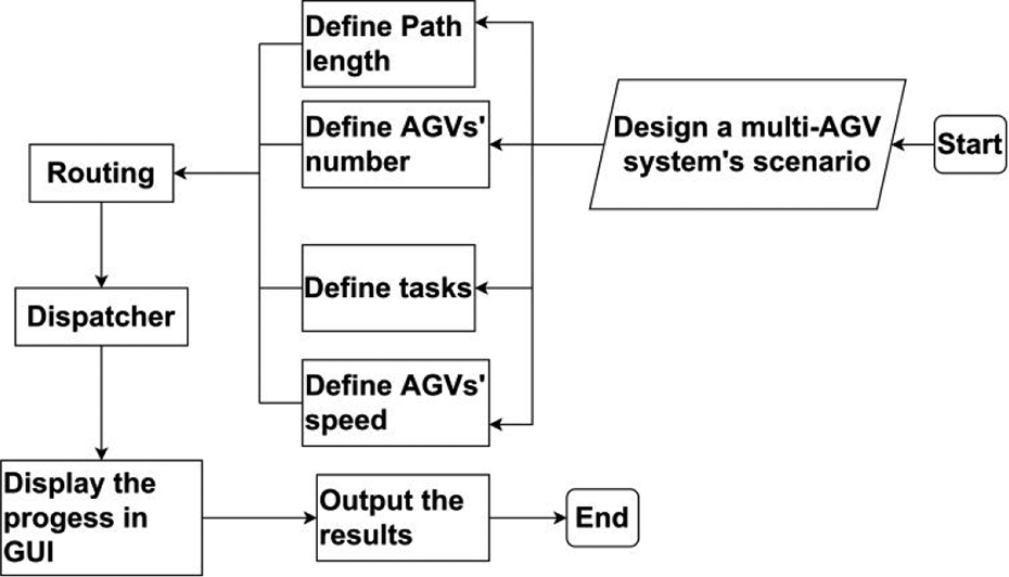
Structure of the simulation platform.
Task allocation is the beginning of the scheduling system. In order to efficiently allocate tasks to the appropriate AGVs, it is necessary to establish appropriate task identification, determine the priority of different tasks, identify the execution status of tasks (being executed, already executed, waiting for execution, canceled, etc.), record the execution process of tasks, and so on. Three modes are raised to optimize the multi-AGV system.
The first mode is called basic mode
The work processing required for goods is proposed periodically by the scheduling system. The task system responsible for task allocation uniformly collects and assigns AGVs for scheduling. Among them, an AGV follows the algorithm of optimizing the shortest path in the process of executing tasks, that is, it traverses all known tasks in the task system and selects the one with the shortest distance from its required movement from these tasks for cargo transfer operation. In the process of pathfinding, an AGV uses A* algorithm for path planning.
Each transportation task contains a list of all stations where the goods need to be processed, as well as the time required for the station to process them. This means that the goods need to be transported to each station in turn and processed at the corresponding time. This task design restores the need to finish the corresponding parts of products on different worktables in the actual factory. When the AGV completes a round of transportation demand according to the task demand (a round of transportation demand refers to loading goods from the current station in the task demand and transporting them to the next station for unloading), the system will not make new route arrangement for the AGV in time. In other words, when unloading goods is completed, if there is no task to be performed in the task system, the AGV will wait at the station by default until the goods are processed at the workstation. After that, the AGV will continue to pick up goods from the site and transport them to the next site for processing. If the AGV encounters another AGV carrying goods to this workstation during the waiting period of the workstation, the AGV in the waiting state will be reassigned by the scheduling system. For example, reassign the AGV in the idle state to a workstation that has completed the processing of certain goods, reload the goods, and continue to transport the goods to the next station according to the task list of the goods. All transportation tasks are regarded as an independent process until all the requirements are completed. The sign of completion of any transportation task is to transport the target goods back to the 11th unloading point of a warehouse. At this time, the system records the cargo throughput plus one.
In general, when the process starts, the scheduling system continues to add new requests for goods processing, including the work site to which the goods need to arrive. After that, the scheduling system reasonably assigns each task to the idle AGV, which follows the shortest path principle and A* algorithm to transport goods. Each cargo handling request will run independently as a process until all requirements are met. This process will actively record the following data: the current work site to arrive, the next work site to arrive, the processing time required by the workstation, and so on. After completing each transportation task, the scheduling system records the throughput and finally ends the process of the transportation task.
The second mode is called no idling mode
The basic theory is consistent with the basic mode, but the difference is that when the cargo is unloaded, the AGV will immediately carry out the next movement operation instead of waiting in place. If there is no waiting task in the task system at this time, the AGV will return to the charging station by default. This mode is proposed to compare the difference between the cargo throughput gap caused by the AGV working at full load and the relatively idle condition.
The third mode is called handover mode
The basic theory is consistent with the basic mode, but the difference is that when the AGV collides with other AGVs in the way of movement, it will give priority to a handover judgment. After delivering the goods, the newly loaded vehicle continues to complete the handling of the goods. The empty vehicle is redistributed by the scheduling system according to the principle of the shortest path. Of course, the target task of the original empty vehicle will be rerecorded to the scheduling system and wait for the scheduling system to redistribute a new idle vehicle to pick up the task.
Furthermore, these modes are based on the A* algorithm to plan the route for the AGVs. The A* algorithm was chosen for the following reasons. A* only focuses on the shortest path from point to point. For the current point on the path, the A* algorithm not only records its cost to the source point but also calculates the desired cost from the current point to the target point, which is a heuristic algorithm. Fewer intermediate nodes need to be extended when searching for the target node, so the algorithm is more efficient.
The A* algorithm is based on Dijkstra’s Algorithm, which is optimized for a single destination, taking into account different movement costs. Although Dijkstra’s Algorithm can find paths to all locations, A* finds the closest one to a location or several locations. It gives priority to paths that appear to be closer to the goal. In contrast, although Dijkstra’s algorithm performs well in finding the shortest path, in the case of multi-AGV scheduling, where multiple AGVs need to be considered simultaneously, using Dijkstra’s algorithm wastes valuable computational resources and computational time by exploring many less promising directions, which is undoubtedly fatal and frightening for the optimization of the entire scheduling system. Similarly, while heuristic search streamlines the exploration directions, for example, in greedy best-first search, we will use the estimated distance from the starting point to the goal for priority queue ordering. The closest position to the goal is explored first. However, when faced with a practical situation with many obstacles, it is difficult to obtain the optimal path, although the computation is fast.
The use of the A* algorithm does not lock its eyes on the task of finding the shortest path, it also takes into account the estimated distance from the starting point to the goal, thus paving the way for the multidimensional situation that needs to be considered during the AGV path planning process. In other words, problems such as deadlock blockage encountered during AGV movement can no longer be reasonably solved by simply planning the shortest path. We can add other conditional functions to the A* algorithm to reasonably predict the time, such as the waiting time at the target station, in order to optimize the scheduling arrangements for the AGV. In summary, A* can be a more suitable algorithm for route planning for multi-AGV scheduling systems. 11
Experimental results and discussion
We conduct experiments to verify the following: (1) The handover mode AGV system has better performance than the traditional AGV system. (2) The designed calculator and simulation platform can work properly and have the potential for further experiments.
Time-cost calculator
By inputting a series of parameters in the calculator, which contains the number of AGVs N, the speed V, the number of tasks M, the scheduling interval T, and path length L, the time-cost calculator can calculate the system’s time cost when all tasks are finished and all AGVs return to the starting point. The time-cost calculator assumes there is only one path in the AGV system. In basic mode, only one AGV is necessary for the system. Meanwhile, the handover time is set to 0 in the time-cost calculator. By changing one of the input parameters and keeping other input parameters stable, Tables 2 –5 and Figure 6 are created.
Basic versus handover interval.

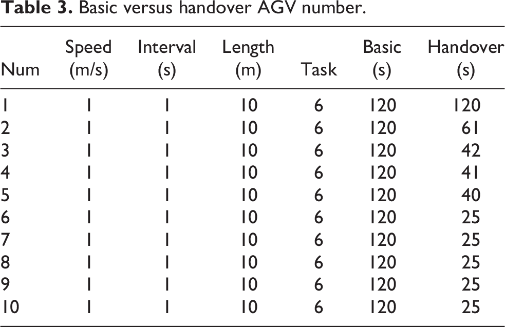
Basic versus handover AGV number.
Basic versus handover tasks.

Basic versus handover length.


One-path time-cost calculator.
In Table 2, we increase the departure interval of each AGV. It can be seen that the longer the departure interval becomes, the longer the system’s time cost will be. In Table 3, we increase the AGVs’ number from 1 to 10. It can be found, in a multi-AGV system in a handover mode, when each AGV’s velocity, each AGV’s departure interval, running distance, and task number of the system do not change, after increasing the AGV’s number to a certain extent, the system’s time cost will not change. In Table 4, we increase the task number from 4 to 16. The system’s time cost is positively correlated with the task number. In Table 5, we increase the path’s length from 1 to 200 m. The system’s time cost is positively correlated with the path’s length.
In Figure 6, it can be seen that in a multi-AGV system using handover mode, each AGV’s scheduling interval time is correlated with the system’s time cost. When other parameters are stable, the number of tasks will not affect the time cost of a multi-AGV system to a certain extent. Each AGV’s velocity is the most important parameter that can affect the multi-AGV system’s time cost. With the growth of each AGV’s velocity, the time cost of a multi-AGV system decreases with the explosive exponential reduction. Furthermore, there exists the best number of AGVs in a multi-AGV system using handover mode. When the number of AGVs achieves such value, it is useless to improve a multi-AGV system’s efficiency by increasing the AGVs’ number.
In Figure 7, what is worth mentioning is that the figure is created based on three paths whose lengths are separately 10, 30, and 50 m. We set up the system to require a total of eighteen tasks to be completed, there are six tasks in each path. After that we set up three scenarios. First, we make the number of AGVs be 6 and make each AGV’s velocity 1 m/s. Then we change each AGV’s interval time to find the relationship between each AGV’s interval time with the multi-AGV system’s time cost. Second, we keep each AGV’s velocity and each AGV’s interval time stable values. Then we change the number of AGVs to find the relationship between AGVs’ number with the multi-AGV system’s time cost. Third, we keep the number of AGVs and each AGV’s interval time be a stable value. Then we change each AGV’s velocity to find the relationship between each AGV’s velocity with the time cost of a multi-AGV system. The conclusions based on the N-path time-cost calculator can be summarized the same as the One-path time-cost calculator.
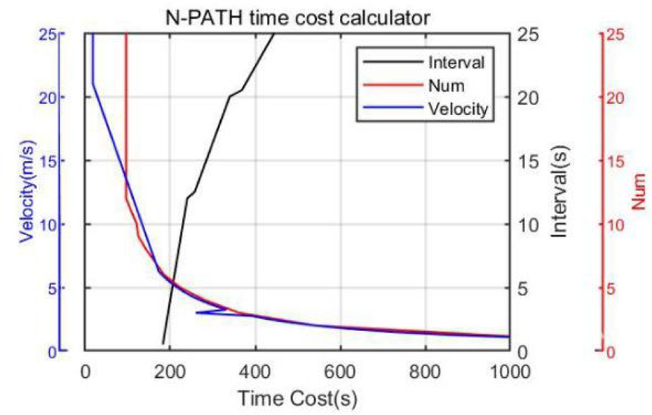
N-Path time-cost calculator.
In summary, experimental results can be summarized as follows: Each AGV’s scheduling interval time is correlated with the system’s time cost. When other parameters are stable, the number of tasks will not affect the time cost of a multi-AGV system to a certain extent. Each AGV’s velocity is the most important parameter that can affect the multi-AGV system’s time cost. With the growth of each AGV’s velocity, the time cost of a multi-AGV system decreases with the explosive exponential reduction. There exists the best number of AGVs in a multi-AGV system using handover mode. When the number of AGVs achieves such value, it is useless to improve a multi-AGV system’s efficiency by increasing the AGVs’ number.
However, the designed calculators still have some limitations. For example, it assumes a relatively ideal environment. The handover time is set to 0. Although this time-cost calculator helps to prove that compared with the basic mode, a system using handover mode can have better performance, a more complicated environment should be considered.
Simulation platform
As mentioned earlier, we create three modes in the simulation platform, which are basic mode, no idling mode, and handover mode. To judge each mode’s performance, we set the number of the AGV and the time to be the same. Then we run the simulation platform and check how many tasks are finished. Meanwhile, to simplify the experimental design of the scheduling system, the following assumptions are considered for the AGV scheduling system. The loading times of the AGVs are all constant values. The speed of the AGVs is a constant value. The operation of the vehicles will not be affected when each vehicle holds different objects. Collisions between vehicles are not allowed, which means that different AGVs cannot occupy common nodes of the inflow path at the same time. Failure of AGVs as well as machines is not considered for the time being.
Because the A* algorithm and the task list can be changed, each mode has a different performance. Therefore, we first test how many tasks can each mode finish in 1500 s. We establish the simulation platform as 10 task points randomly selected from 10 task points for each handling task. There are six AGVs in the simulation. The results can be seen in Table 6. It can be seen that compared with the other two modes, the handover mode finishes the most tasks at the same time.
Different modes’ performance in 1500 s.

Then, we change the time. We test each mode’s performance 10 times at the same time to get an average value. After that testing results are established in Figure 8. It gives an illustrative example to demonstrate how different modes perform in different situations. Figure 8(a) makes 10 AGVs run to 10 workstations to finish the tasks in 700, 900, 1100, 1300, 1500, and 1700 s. Figure 8(b) makes 10 AGVs run to 10 workstations to finish the tasks in 700, 900, 1100, 1300, 1500, and 1700 s. Figure 8(c) makes 10 AGVs run to 10 workstations to finish the tasks in 700, 900, 1100, 1300, 1500, and 1700 s. Figure 8(d) makes 10 AGVs run to 10 workstations to finish the tasks in 700, 900, 1100, 1300, 1500, and 1700 s. Figure 8(e) makes 10 AGVs run to 10 workstations to finish the tasks in 700, 900, 1100,1300, 1500, and 1700 s.

Testing results.
In summary, by using the handover method in a multi-AGV system, the system’s performance can be improved. However, these conclusions obtained so far are analyzed in the overall context. This is because when looking deeper into the data from each experiment, we can see that not all cases in this setting (with different task release intervals) show negative optimization when the handover algorithm is added. In fact, when a task system releases a task at a suitable time for the handover algorithm, it also makes that scheduling system outperform other scheduling systems. Second, as the handover algorithm makes it necessary for the AGV to have handover time when handing over the goods and for the workstation to have processing time when handing the goods, the choice of these times will also affect the final experimental results to some extent.
Conclusion
We present two multi-AGV time-cost calculators and a multi-AGV scheduling simulation platform. A scheduling optimization method is also raised. Related experiments and tests have been done. The superiority of the raised scheduling optimization method has been proved. Meanwhile, parameters that can influence the system’s performance have been tested. The handover mode is better than the basic mode. Most parameters are correlated with the system’s time cost except the number of AGVs. There exists a best number of AGVs in a multi-AGV system using handover mode. Therefore, the handover method should be paid more attention to be applied in multi-AGV systems’ scheduling optimization area.
The designed multi-AGV scheduling simulation platform visualizes to a certain extent the operation flow of the whole system and includes the A* algorithm and handover method. It provides a direction for solving the AGV scheduling problem. In addition, experiments are conducted to compare and test the optimization methods used in this project. The maximum throughput that can be achieved in practice and the overall power consumption of the AGVs are derived. Continuous improvement (adjusting parameters, correcting algorithms) is carried out on the tests, the tests are repeated, and the results are recorded. Finally, a comparison of the performance of the different scheduling systems is achieved. After statistical analysis of the results, it was determined that the cooperative scheduling system for this research project obtained good performance.
The future work is to expand our work. We plan to optimize the current time-cost calculator so that it can deal with the N-path situation. Meanwhile, we plan to add a parameter handover time to the time-cost calculator with other specific parameters to better test what will influence a multi-AGV system and how can they influence the system. We plan to optimize the current simulation platform so that it can simulate and schedule robots with different capabilities, apply different path planning and obstacle avoidance algorithms, and add more specific conditions to make the simulation environment close to the real scene. Thus, the deployed robot system can be tested with more applicability.
Footnotes
Declaration of conflicting interests
The author(s) declared no potential conflicts of interest with respect to the research, authorship, and/or publication of this article.
Funding
The author(s) disclosed receipt of the following financial support for the research, authorship, and/or publication of this article: This research was partially supported by the Suzhou Municipal Key Laboratory Broadband Wireless Access Technology (BWAT).