Neural ordinary differential gray algorithm to forecasting models of controlled systems

Abstract

Due to the feasibility of the gray model for predicting time series with small samples, the gray theory is well investigated since it is presented and is currently evolved in an important manner for forecasting small samples. This study proposes a new gray prediction criterion based on the neural ordinary differential equation, which is named the neural ordinary differential gray mode. This neural ordinary differential gray mode permits the forecasting model to be learned by a training process which contains a new whitening equation. It is needed to prepare the structure and time series, compared with other models, according to the regularity of actual specimens in advance, therefore this model of neural ordinary differential gray mode can provide comprehensive applications as well as learning the properties of distinct data specimens. To acquire a better model which has highly predictive efficiency, afterward, this study trains the model by neural ordinary differential gray mode using the Runge–Kutta method to obtain the prediction sequence and solve the model. The controller establishes an advantageous theoretical foundation in adapting to novel wheels and comprehensively spreads the utilize extent of mechanical elastic vehicle wheel.

Introduction

In the last 5 years some methods have appeared to detect errors, interference effects, modeling errors, various uncertainties in real systems, and so on. For example, Xin et al. ¹ and Cheng et al. ² also proposed the linear matrix inequality (LMI) technique, which provides sufficient conditions to guarantee the existence of asynchronous error detection. Xu et al. ³ found the method suitable for the applications, and the results analyzed the stability of the state-dependent step delay network for gene regulation and proposed suitable sufficient conditions based on model transformation and LMI, resistance is an important component of the control system, but optimal control cannot guarantee fundamental robustness. ⁴ It is well known that SM control is an effective tool to improve the resilience of control systems regardless of external disturbances or parameter changes. To solve the singularity and flutter problems, a systematic control scheme for SST was sought. ⁵ To control AS, I/O compensation 11 in slip mode is suggested. However, SM control does not provide AS with optimal nominal capacity. In addition to robustness, optimal suspension control has been incorporated into the slider position control to improve optimization possibilities. ⁶

For Taylor-corrected linear systems containing nonintegral non-quadratic terms, an optimal slide position control is pursued to improve the optimal control problem, ⁷ and a linear quadratic strategy for optimal slide position supply for logistics systems is proposed. ⁸ Currently, many SM-optimized control methods have been used to design vehicle steering suspension. For example, an optimal SM controller with feedback/feedback in the control system has been proposed. ⁹ Unfortunately, these controls do not achieve the truly optimal possibilities for wide suspension. ⁴ Furthermore, it is a classic nonlinear mechanical suspension system with complex dynamics that can cause unacceptable ill effects on passengers and drivers. ² Therefore, an adaptive control tracking method for nonlinear tuning of quadratic systems is proposed to achieve excellent suspension performance. ¹⁰ Based on the T-S fuzzing method, in nonlinearly controlled fuzzy systems, a robust nonlinear predictive multivariate control is proposed. ¹¹ Therefore, nonlinear elements of shock absorbers and springs must be anticipated when designing useful ride control models to compensate for nonlinear effects and provide increased drivability of large-scale vehicles.

In practice, few samples are usually available. For example, China has less than 30 oil consumption samples per year so far, so this is also an important area where it can make accurate predictions from a small number of samples. Currently, there are many methods to make predictions with a small number of samples, for example, fuzzy theories, ^{12 –16} neural systems, ^{17 –20} and graphic systems science. ^{21 –23} By better understanding the law of the data, the gray system theory can reduce to a certain extent the source of uncertainty generated by a small number of samples to more effectively predict small sample data. The gray theory approach was developed by Ju-Long ²⁴ to solve uncertainty problems. The basic model is the so-called GM model (1, 1). Because this gray theoretical model is efficient, simple, and inexpensive, it has been widely used in recent years in research to forecast short-term time series, including vehicle flows and prices, and oil production. ^{25 –28} As a result of further research on GM models (1, 1), many new gray models were created. ^29,30 These models take into account the disadvantages of this GM model (1, 1), so we usually get a higher accuracy.

When it comes to the gray pattern search, some researchers rely on the pattern method, combine it with the idea of a single pattern and arrive at the pattern with a discrete gray pattern (DGM) (1, 1). ³⁰ When the specimen data are homogenized, DGM models carry out poorly; nonetheless, thanks to ³¹ propose an NDGM model which extends it to heterogeneous models. ¹⁹ The real specimen data cannot usually meet the homogeneous property, due to the GM(1, 1) model being a homogeneous kind model, thus extremely restricts its feasibility. The NGM(1, 1, k) model by Chen and Chen ³² was introduced to correct these shortcomings. Nevertheless, this model introduces some novel methods. For instance, when it comes to predicting real-time series, actually the NGM model is not as powerful as the GM(1, 1) model, even though it can attain greater accuracy on specimens by uneven exponential properties. Thus, the ONGM model was provided by Chen and Meng ³³ to solve that problem. Duan et al. provided a gray forecasting model with a point function by combining the gamma function with the SIGM model, which is called the FSIGM model. ^34,35 Due to nuclear methods being useful for solving nonlinear problems, some researchers have taken advantage of these properties and proposed gray models based on nuclear methods. ^{36 –43} The method allows these criteria to effectively forecast nonlinear sequences.

Neural ordinary differential equation (NODE) is a novel nervous system proposed by Si-feng. ⁴⁴ It makes a single transition ⁴⁵ successive between different layers of a remaining network; in this way, the whole network becomes successive and can be adjusted with standard differential equations. NODE has aroused the interest of many researchers because it relates differential equations to neural networks (NNs), which is a novel area of NNs. NODE is currently used in various mechanistic and in-depth research studies. ^{46 –56} According to Lei et al., ⁵⁷ the gray algorithm is used for the modeling in energy and economics, however, the gray systems could be combined with the fuzzy and artificial intelligence adjusting controlled design for the real-world application in nonlinear systems.

The main contributions and innovations compared with the existing results have been highlighted that gray modeling control and mechanical LMI criterion have been combined to solve nonlinear numerical control inequalities for real-world demonstrations. This study learns that lots of gray models require a preliminary definition of the concept and configuration of the white balance equation. The parameters can be assessed with optimization approaches, for example, least square, according to the bleaching equation. Then, by figuring out this differential equation, the predicted procedure can be calculated. But it cannot guarantee that this terminology as well as configuration of the kind model defined correspond to the properties of these actual data if they lack appropriate knowledge. Secondly, although gray models are adequate for predicting few specimen sizes, their estimation method is based on the risk-reduced least square empirical parameters, which ensures that predictions are made only for bigger specimen sizes. Therefore, while in the condition of few specimens, the probability of obesity according to the least squares method is high. To address these issues, in collaboration with NODE, this document presents a new gray prediction model, whereby NODE the bleaching equation is defined. As for the model, it is not required to offer an explicit configuration and terminology, as the optimum models are acquired through a learning procedure that can be resolved with the Runge–Kutta approach. Thus, for data with different distributions the NODGM model can be used. Due to the model training is according to a sloping function, by controlling the loss threshold or the iteration numbers, the NODE can be trained to decrease the risk of obesity as well as furthermore enhance the predictive efficiency of this model which was trained.

The rest of the article has been arranged as follows: The second section presents these essentials of the GM(1, 1) model. We represent the theory of NODGM and NODE in the third section. The fourth section presents numerical cases of prognostics with gray models in different gross forecasting models. The final section concludes this study and summarizes the presentation.

GM methodology

As the research and development trend in gray system theory, numerous innovative models are provided on the basis of GM(1, 1) model. At the present, this study will describe the modeling procedure and parameter evaluation approach of this fundamental model (GM(1, 1) model).

Here represents the series (1)

$\begin{array}{c}\left(x^1\left(1\right),x^1\left(2\right),x^1\left(3\right),\dots ,x^1\left(n\right)\right)\end{array}$

1

The gray model adopts the 1-AGO series to establish the forecasting system instead of the sequence of raw data, such as Figure 1. It is a 1-order generation (1-AGO) accumulated queue.

Figure 1.

The difference of transformation between a residual network and an ODE network. ODE: ordinary differential equation.

$\begin{array}{c}\left(x^0\left(1\right),x^0\left(2\right),x^0\left(3\right),\dots ,x^0\left(n\right)\right)\end{array}$

2

Here we define the GM(1, 1) model as follows

$\begin{array}{c}{x}^0\left(1\right)+\alpha z^1\left(t\right)=b,\hspace{1em}t=2,3,\dots ,n\end{array}$

3

in which $x^1\left(k\right)={\displaystyle {\sum }_{i=1}^k{x}^0\left(t\right)},\hspace{0.17em}{z}^1\left(k\right)=\frac{1}{2}\left(x^1\left(k-1\right)+x^1\left(k\right)\right),\hspace{0.17em}k=2,3,\dots ,k$

In the end, the predictive values for the raw data ${\widehat{x}}^0\left(t\right)$ will be collected through the equation as follows

$\begin{array}{c}{\widehat{x}}^0\left(t\right)=-{\widehat{x}}^1\left(t-1\right)+{\widehat{x}}^1\left(t\right),\hspace{1em}t=2,3,\dots ,n\end{array}$

4

Preliminary proposed methodology

An NODEs

NODE is discriminated against from a single NN, it is a novel branch of a NN. As displayed in Figure 1, the remaining network possesses a distinct transform function f(h(t), θ(t)) in between every layer; thus, the entire networks express a sequence of diverse input transformations of the NN. Of course, the latent state path is the dotted line shown in the top row of Figure 1, and the weights are stored in each layer of network. As the depth between the networks rise rapidly, the derived resources needed to maintain the site become expensive. But in NODE, this transformation from data input to data output are both continuous, thus the curve h(t) presents a smooth mild curve, which is displayed on the last line in Figure 1, which presented that the network itself can be corrected with standard differential equations (ordinary differential equation (ODE)).

In terms of such a continuous NN, this study applies common NN training methods to train ODE with ODE symptoms. Then only save the ODE parameters regardless of the depth of the NN. By resolving the ODE with the preliminary value which can calculate the h(t) value for any t.

Actually, NODE could be considered as a particular residual network, their configuration is a series of residual blocks shown in Figure 2. With comparison to the criterion residual network, in the ODE network each block possesses the identical f. From the residual block that presents the h(t) input and h(t + 1) output satisfies

$\begin{array}{c}h\left(t+1\right)=f\left(h\left(t\right),{\theta }_t\right)+h\left(t\right) \hspace{1em}\text{or}\hspace{1em}h\left(t+1\right)=kf\left(h\left(t\right),t,\theta \right)+h\left(t\right)\end{array}$

5

in which k is the step size and presents that there is only one equilibrium solution as it has a proper function f(t, θ, h(t)) equated to the output signal from the normal remaining network on the corresponding layer. So ODE is considered as a successive remaining network, which is called the ODE NN.

Figure 2.

The block in residual.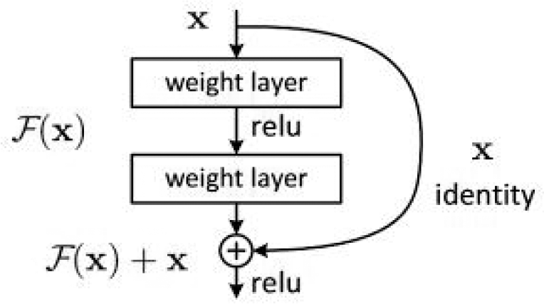

In the NODE condition, this function f embodies the variables which could be produced. As with a single nervous system, the transmission of backscatter needed for NODE training is followed. Euler’s method described above is only an exact 1-series method—a number of higher order ODE solution methods have been provided recently. Such as, the Runge–Kutta approach ³⁸ is a common method for solving ODE, which has better accurateness than Euler’s approach. In this article, the Runge–Kutta approach is considered as black box while resolving ODE, called ODESolver. The procedure for solving Runge–Kutta approach is from the initial value under an ODE problem

$\begin{array}{c}{y}^{\prime }=f\left(x,y\right), \hspace{1em}y\left(x_0\right)=y_0,\hspace{1em} x\in \left[x_0,x_f\right]\end{array}$

6

This Runge–Kutta approach is a constant step size, which makes it less flexible than the adjusted step size method. ⁵⁸ Thus, this study could call ODESolver the ODE network redirection

$\begin{array}{c}\begin{array}{c}h\left(t\right)=h\left(t_0\right)+{\displaystyle {\int }_{t0}^{t}f\left(t,\theta ,h\left(t\right)\right)\text{d}t}\\ =\text{ ODESolver }\left(h\left(t\right),t,h\left(t_0\right),f\left(\left(h\left(t\right),t,\theta \right),\theta \right)\right)\end{array}\end{array}$

7

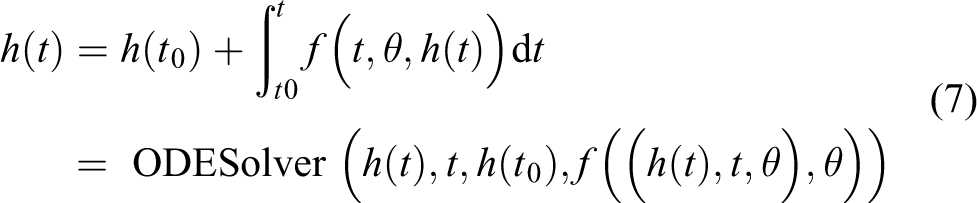
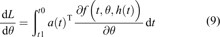
ODESolver calculates an answer according to the start value h(0), θ, the initiate point t0 as well as the end point t, as the answer of ODE in the equation. By calling the ODESolver, it can be calculated. Then, from the function f(t, θ, h(t)) could readily get the part of f relative to the numerical hidden layer h. Use ODESolver to compute the transformation result (h(t0), t0, θ, t), that can directly calculate the end position a(tn) = ∂L. Then it can use ODESolver to resolve equation (7) and calculate entire adjacent states backward, initiating from the ultimate continuous condition a(tn)

$\begin{array}{c}a\left(t\right)=\text{ ODESolver }\left(a\left(t_n\right),t,\frac{\partial f\left(h\left(t\right),t,\theta \right)}{\partial h}\right)\end{array}$

8

While acquiring $a\left(t\right)$ by equation (8), the fractional $\frac{\partial L}{\partial \theta }$ requires to be acquired to renovate the coefficient θ. The variable $\frac{\text{d}L}{\text{d}\theta }$ can be obtained by resolving the integral as follows

$\begin{array}{c}\frac{\text{d}L}{\text{d}\theta }={\displaystyle {\int }_{t1}^{t0}a{(t)}^{\text{T}}\frac{\partial f\left(t,\theta ,h\left(t\right)\right)}{\partial \theta }\text{d}t}\end{array}$

9

We finally could use the dL/dθ slope to renovate the parameters and accomplish the regeneration procedure.

Actually, to insert a vector and then release another vector of a certain size is a single nervous system’s real role. At the same time, since the network itself is a complex multilayered feature with distinguishability, it can update parameters by spreading forward and backward. In this way, a single NN could be incorporated into standard differential equations, as presented in the “NODGM statement” section. Learn more about the derivative procedure of equations. Equations (7) to (9) are included in Annex B to the NODE. ^{59 –61}

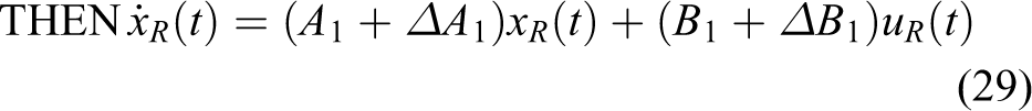
NODGM statement

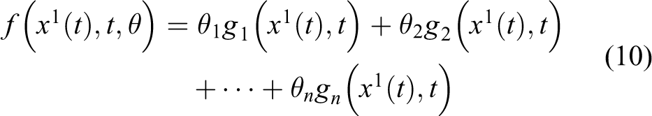
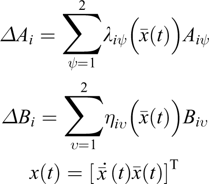
In the section, the study introduces a novel gray model that is called NODGM. Rather than estimating the corresponding differential model ^{62 -65} by solving the parameters with the least squares approach, the NODGM model defines the function fx1(t), t, θ, which replaces estimate 1 with t. The AGO family can treat the bleaching equation as a knot, and by teaching its ODE a better predictive model can be obtained.

Whereas assume the condition of f is a function of t and x1(t), in the NODGM model, the coefficient θ is a parameter. Thus, this function of f could be as follows

$\begin{array}{c}f\left(x^1\left(t\right),t,\theta \right)={\theta }_1{g}_1\left(x^1\left(t\right),t\right)+{\theta }_2{g}_2\left(x^1\left(t\right),t\right)+\cdots +{\theta }_n{g}_n\left(x^1\left(t\right),t\right)\end{array}$

10

in which $f\left(x^1\left(t\right),t,\theta \right)$ presents a train of transformations in simulation about t and $x^1\left(t\right)$ . The discrete NN (DNN) could be also regarded as a train of numerical transformations under its input. Thus, to approximate the function f in which could derive a DNN whose input by $x^1\left(t\right)$ . Let $h\left(t\right)=x^1\left(t\right)$ , and then the formula in whitening of the numerical model will be derived as a numerical NODE

$\begin{array}{c}f\left(\theta ,t,h\left(t\right)\right)=\frac{\text{d}h\left(t\right)}{\text{d}t}\end{array}$

11

By a DNN, where the function f is defined, and θ is the weight value. By transforming the NN that derives the numerical function f, so the model can possess various patterns such as nonhomogeneous, homogeneous, nonlinear, or linear. Given the preliminary value time span tspan and θ, h(0), then that can utilize an ODESolver to calculate the forecasting procedure H

$\begin{array}{c}H=\text{ ODESolver }\left(h\left(t\right),t,f\left(h\left(t\right),t,\theta \right),h\left(0\right),\text{ tspan},\theta \right)\\ =\left[h\left(0\right),\widehat{h}\left(1\right),\dots ,\widehat{h}\left(n-1\right)\right]\end{array}$

12

in which tspan = [0, 1,…, n − 1]. We develop the loss function to train the numerical NODE to optimize the coefficient θ

$\begin{array}{c}L={\Vert H-X^0\Vert }_2^2={\displaystyle \sum }_{t=0}^{\text{n}}{\left(\widehat{h}\left(t\right)-h\left(t\right)\right)}^2\end{array}$

13

Therefore, the NODGM model is based on the slope for parameter formation, not the least squares approach. Meanwhile, since the function of this bleaching equation has been derived by the NN, prior knowledge is incorporated into the network design, which significantly reduces the time required to practice ODE.

Case study

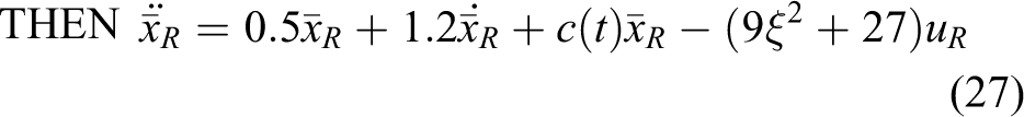
If these time steps are small enough, entire conditions in the system are continuous time instances. DGM step (2, 1) should ensure that follow-up is consistent and limited. The control adapts to the gray oracle signal reception conditions and possesses adaptive force control for tracking the movement produced by the ideal damping hybrid control to study the movement of the mechanical elastic vehicle wheel which is equipped with an active suspension of the vehicle.

To check control circuit, the first step in DGM(2, 1) has been corrected, use trailer to simulate digital random motion data set, predict signal sequence 6 will be set to 0.001s, then design Simulink step to design two standard tunnels A (impulse and steps) to illustrate the effectiveness of the proposed monitoring. This road connection, which works on the rear and front wheels, has a certain delay that corresponds to the vehicle’s speed and wheelbase. The measurable coefficients for the simulator are shown in Table 1.

Table 1.

Measurable program factors.

Values	Parameters	Units	Values	Parameters	Units
750	M	kg	19,650	a21	N·m1
1130	Iy	kg·m2	1	a22	N·m2
45	m 1	kg	1	a23	N·m3
45	m 2	kg	1290	b21	N·s·m1
9.8	g	m·s2	1	b22	N·s2·m2
1.2	a	m	1	b23	N·s3·m3
1.7	b	m	0.003	d	M
15	v	m·s1	2100	Csky1	N·s·m1
19,600	a11	N·m1	2100	Csky2	N·s·m1
1	a12	N·m2	2100	Csky3	N·s·m1
1	a13	N·m3	2100	Csky4	N·s·m1
1290	b11	N·s·m1	15	k 1	—
1	b12	N·s2·m2	15	k 2	—
1	b13	N·s3·m3	—	—	—

The difference between the GDM(2, 1) model prediction and the exact data is so small, particularly while the development is small relatively. The GDM(2, 1) model’s tracking error will be slightly larger if the data change remarkably; but it still suffices the qualification for engineering work. Thus, in DGM(2, 1) reliable quality can also be determined. The matrices weighted in the hidden layer and output have been indicated by W ² and W ¹. After training the BP algorithm, this weighted factor can be collected in the following equations

$\begin{array}{c}{v}_r^1=W_{1r}^{1}x\left(k\right)+W_{2r}^{1}x\left(k-1\right)+W_{3r}^{1}u\left(k\right)\\ v_1^2=W_{11}^{2}T\left(v_1^1\right)+W_{21}^{2}T\left(v_2^1\right)+W_{31}^{2}T\left(v_3^1\right),x\left(1+k\right)=T\left(v_1^2\right)\\ x\left(1+k\right)=\left(h_{11}^2\left(k\right)g_1+h_{12}^2\left(k\right)g_2\right)v_1^2={\displaystyle \sum }_{i=1}^2{h}_{1i}^2\left(k\right)g_i{v}_1^2\end{array}$

14

In addition, based on matrix numbering, the NN model could be developed in the LDI indications as follows

$\begin{array}{c}x\left(1+k\right)={\displaystyle \sum }_{i=1}^{16}{h}_i\left(k\right)\left\{A_{i}x\left(k\right)+B_{i}u\left(k\right)\right\}\end{array}$

15

The above equation proves that the nonlinear term can be confined by an upper bound and a lower bound. According to the interpolation algorithm, the nonlinear term can be represented by the following equation

$\begin{array}{c}{\overline{x}}^3\left(t\right)u=\frac{\left[M_1\left(\overline{x}\left(t\right)\right)\times \left(-27\right)+M_2\left(\overline{x}\left(t\right)\right)\times \left(27\right)\right]}{M_1\left(\overline{x}\left(t\right)\right)+M_2\left(\overline{x}\left(t\right)\right)}u\end{array}$

16

Assume that

$\begin{array}{c}{M}_1\left(\overline{x}\left(t\right)\right)+M_2\left(\overline{x}\left(t\right)\right)=1\end{array}$

17

and

$M_1\left(\overline{x}\left(t\right)\right)\in \left[\begin{array}{cc}0& 1\end{array}\left],\hspace{1em}{M}_2\left(\overline{x}\left(t\right)\right)\in \right[\begin{array}{cc}0& 1\end{array}\right]$

Then, by solving (6.3) and (6.4), $M_1\left(\overline{x}\left(t\right)\right)$ and $M_2\left(\overline{x}\left(t\right)\right)$ are obtained as follows:

$\begin{array}{c}{M}_1\left(\overline{x}\left(t\right)\right)=0.5-\frac{{\overline{x}}^3\left(t\right)}{54},\hspace{1em}{M}_2\left(\overline{x}\left(t\right)\right)=0.5+\frac{{\overline{x}}^3\left(t\right)}{54}\end{array}$

18

The uncertain nonlinear system can be described by the following T-S fuzzy model with uncertainty

Rule 1:

IF $\overline{x}$ is M ₁

$\text{THEN}\hspace{0.17em}\hspace{0.17em}\begin{array}{c}\ddot{\overline{x}}=0.5\overline{x}+c\left(t\right)\overline{x}+1.2\dot{\overline{x}}-27u\end{array}$

19

Rule 2:

IF $\overline{x}$ is M ₂

$\text{THEN}\hspace{0.17em}\hspace{0.17em}\begin{array}{c}\ddot{\overline{x}}=0.5\overline{x}+c\left(t\right)\overline{x}+1.2\dot{\overline{x}}+27u\end{array}$

20

By introducing matrix representation, it can be rewritten as follows

Rule 1:

IF $\overline{x}\left(t\right)$ is M ₁

$\text{THEN }\begin{array}{c}\dot{x}\left(t\right)=\left(A_1+\text{Δ}{A}_1\right)x\left(t\right)+\left(B_1+\text{Δ}{B}_1\right)u\left(t\right)\end{array}$

21

Rule 2:

IF $\overline{x}\left(t\right)$ is M ₂

$\text{THEN }\begin{array}{c}\dot{x}\left(t\right)=\left(A_2+\text{Δ}{A}_2\right)x\left(t\right)+\left(B_2+\text{Δ}{B}_2\right)u\left(t\right)\end{array}$

22

where

$\begin{array}{c}\Delta A_i={\displaystyle \sum }_{\psi =1}^2{\lambda }_{i\psi }\left(\overline{x}\left(t\right)\right)A_{i\psi }\\ \Delta B_i={\displaystyle \sum }_{\upsilon =1}^2{\eta }_{i\upsilon }\left(\overline{x}\left(t\right)\right)B_{i\upsilon }\\ x\left(t\right)={\left[\begin{array}{cc}\dot{\overline{x}}\left(t\right)& \overline{x}\left(t\right)\end{array}\right]}^{\text{T}}\end{array}$

$\begin{array}{l}{A}_1=\left[\begin{array}{cc}1.2& 0.5\\ 1& 0\end{array}\right],\hspace{1em}{B}_1=\left[\begin{array}{c}-27\\ 0\end{array}\right]\\ A_2=\left[\begin{array}{cc}1.2& 0.5\\ 1& 0\end{array}\right],\hspace{1em}{B}_2=\left[\begin{array}{c}27\\ 0\end{array}\right]\end{array}$

$\begin{array}{l}{A}_{11}=A_{21}=\left[\begin{array}{cc}0& -0.4\\ 0& 0\end{array}\right],\hspace{1em}{A}_{12}=A_{22}=\left[\begin{array}{cc}0& 0.4\\ 0& 0\end{array}\right]\\ B_{11}=B_{21}=B_{12}=B_{22}=\left[\begin{array}{c}0\\ 0\end{array}\right]\end{array}$

Notice that

$\begin{array}{l}{\lambda }_i\left(\overline{x}\left(t\right)\right)\ge 0,\hspace{1em}i=1,2,\hspace{0.17em}\psi =1,2\\ {\displaystyle \sum }_{\psi =1}^2{\lambda }_{i\psi }\left(\overline{x}\left(t\right)\right)=1\end{array}$

$\begin{array}{l}{\eta }_i\left(\overline{x}\left(t\right)\right)\ge 0,\hspace{1em}i=1,2,\hspace{0.17em}\hspace{0.17em}\upsilon =1,2\\ {\displaystyle \sum }_{\upsilon =1}^2{\eta }_{i\upsilon }\left(\overline{x}\left(t\right)\right)=1\end{array}$

Hence, the overall fuzzy model with uncertainty $F\left(0;0\right)$ is

$$\begin{gathered} \dot{x}\left(t\right)={\displaystyle \sum }_{i=1}^2{\displaystyle \sum }_{\psi =1}^2{\displaystyle \sum }_{\upsilon =1}^2{M}_i\left(\overline{x}\left(t\right)\right){\lambda }_{i\psi }\left(\overline{x}\left(t\right)\right){\eta }_{i\upsilon }\left(\overline{x}\left(t\right)\right) \\ \left\{\left(A_i+A_{i\psi }\right)x\left(t\right)+\left(B_i+B_{i\upsilon }\right)u\left(t\right)\right\} \end{gathered}$$

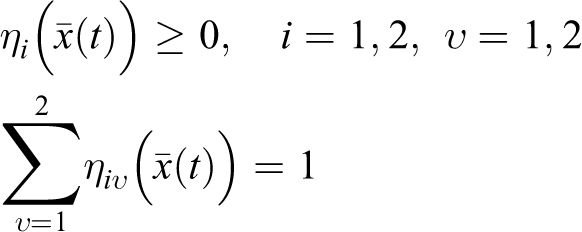
The fuzzy sets $M_1\left(\overline{x}\left(t\right)\right)$ and $M_2\left(\overline{x}\left(t\right)\right)$ are illustrated in Figure 3.

Figure 3.

Fuzzy sets $M_1\left(\overline{x}\left(t\right)\right)\text{ and }{M}_2\left(\overline{x}\left(t\right)\right)$ .

According to the above equations, we know that the pairs $\left(\begin{array}{cc}{A}_1& B_1\end{array}\right)$ and $\left(\begin{array}{cc}{A}_2& B_2\end{array}\right)$ are controllable. Hence, two local fuzzy controllers are designed to stabilize systems. The fuzzy controller is designed via the PDC scheme to decide two feedback gains in its consequent parts. The feedback gains F ₁ and F ₂ can be obtained by the linear quadratic optimal control technique as follows

$F_1=\left[\begin{array}{cc}-1.0824& -1.0187\end{array}\right],\hspace{1em}{F}_2=\left[\begin{array}{cc}0.7428& 0.9316\end{array}\right].$

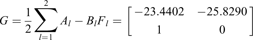
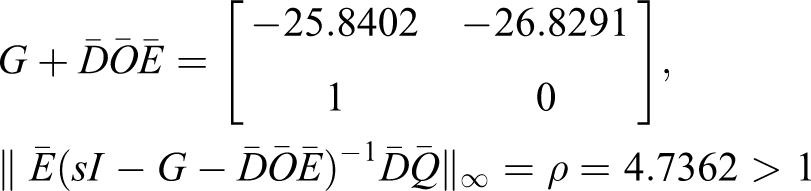
The Riccati equation for linear continuous systems is used to design these feedback gains because the local fuzzy controllers are designed based on T-S fuzzy model without uncertainty. According to the above conditions, we can obtain the matrix G as follows

$G=\frac{1}{2}{\displaystyle \sum }_{l=1}^2{A}_l-B_l{F}_l=\left[\begin{array}{cc}-23.4402& -25.8290\\ 1& 0\end{array}\right]$

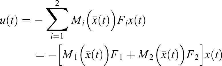
The final output of the fuzzy controller is

$$\begin{gathered} u\left(t\right)=-{\displaystyle \sum }_{i=1}^2{M}_i\left(\overline{x}\left(t\right)\right)F_{i}x\left(t\right) \\ =-\left[M_1\left(\overline{x}\left(t\right)\right)F_1+M_2\left(\overline{x}\left(t\right)\right)F_2\right]x\left(t\right) \end{gathered}$$

We can derive the closed-loop uncertain fuzzy system $F\left(C;0\right)$

$$\begin{gathered} \dot{x}\left(t\right)={\displaystyle \sum }_{i=1}^2{\displaystyle \sum }_{j=1}^2{\displaystyle \sum }_{\psi =1}^2{\displaystyle \sum }_{\upsilon =1}^2{M}_i\left(\overline{x}\left(t\right)\right)M_j\left(\overline{x}\left(t\right)\right) \\ {\lambda }_{i\psi }\left(\overline{x}\left(t\right)\right){\eta }_{i\upsilon }\left(\overline{x}\left(t\right)\right)\left\{A_i-B_i{F}_j+A_{i\psi }-B_{i\upsilon }{F}_j\right\}x\left(t\right) \end{gathered}$$

From equations (20) to (22), we have

$$\begin{gathered} G+\overline{D}\overline{O}\overline{E}=\left[\begin{array}{cc}-25.8402& -26.8291\\ 1& 0\end{array}\right], \\ \parallel \overline{E}{(sI-G-\overline{D}\overline{O}\overline{E})}^{-1}\overline{D}\overline{Q}{\parallel }_{\infty }=\rho =4.7362>1 \end{gathered}$$

Hence, the closed-loop uncertain fuzzy system is not quadratically stable. This implies that the fuzzy controller cannot stabilize the fuzzy model with uncertainty $F\left(0;0\right)$ . Simulation results of the closed-loop uncertain nonlinear system $N\left(C;0\right)$ are shown in Figure 4.

Figure 4.

Simulated controlled modeling uncertain nonlinear system $N\left(C;0\right)$ .

Subsequently, we attempt to improve the stability of the closed-loop uncertain nonlinear system $N\left(C;0\right)$ by injecting a periodic symmetrical $d\left(t\right)$ with sufficiently high frequency. Notice that the dither signal is injected just in front of the nonlinearity. The uncertain system $N\left(0;d\right)$ is described as follows

$\ddot{\overline{x}}=0.5\overline{x}+1.2\dot{\overline{x}}+c\left(t\right)\overline{x}+{(d+\overline{x})}^{3}u$

To analyze the uncertain dithered model, the corresponding uncertain relaxed model is established as the following equation

$$\begin{gathered} {\ddot{\overline{x}}}_R=0.5{\overline{x}}_R+1.2{\dot{\overline{x}}}_R+c\left(t\right){\overline{x}}_R+\left[{\alpha }_1{\left({\beta }_1+{\overline{x}}_R\right)}^3 \\ +{\alpha }_2{\left({\beta }_2+{\overline{x}}_R\right)}^3\right]u_R \end{gathered}$$

with

${\alpha }_1=0.5,\hspace{1em}{\alpha }_2=1-{\alpha }_1=0.5,\hspace{1em}{\beta }_1=-{\beta }_2=\xi$

where ${\alpha }_i$ and ${\beta }_i$ are the random parameters and $\xi$ is a real constant number, which allows us to rewrite the uncertain relaxed model $N_R\left(0;0\right)$ as follows

$\begin{array}{c}{\ddot{\overline{x}}}_R=0.5{\overline{x}}_R+1.2{\dot{\overline{x}}}_R+c\left(t\right){\overline{x}}_R+\left(3{\xi }^2{\overline{x}}_R+{\overline{x}}_R^3\right)u_R\end{array}$

23

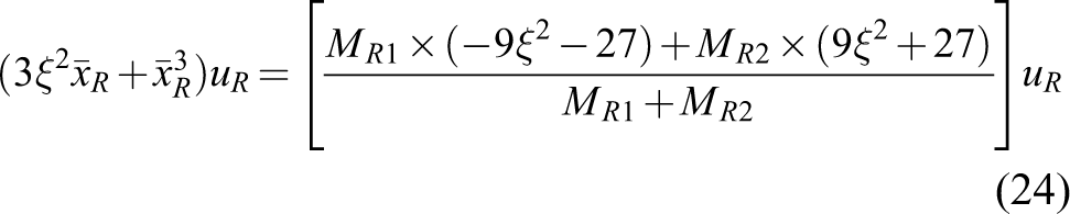
The nonlinear term of this system is $\left(3{\xi }^2{\overline{x}}_R+{\overline{x}}_R^3\right)u_R$ , which satisfies the following condition for ${\overline{x}}_R\in \left[\begin{array}{cc}-3& 3\end{array}\right]$

$\left(-9{\xi }^2-27\right)u_R\le \left(3{\xi }^2{\overline{x}}_R+{\overline{x}}_R^3\right)u_R\le \left(9{\xi }^2+27\right)u_R$

Similarly, the nonlinear term can be represented as follows

$\begin{array}{c}\left(3{\xi }^2{\overline{x}}_R+{\overline{x}}_R^3\right)u_R=\left[\frac{M_{R1}\times \left(-9{\xi }^2-27\right)+M_{R2}\times \left(9{\xi }^2+27\right)}{M_{R1}+M_{R2}}\right]u_R\end{array}$

24

where

$\begin{array}{c}{M}_{R1}+M_{R2}=1\end{array}$

25

and

$M_{R1}\in \left[\begin{array}{cc}0& 1\end{array}\left],\hspace{1em}{M}_{R2}\in \right[\begin{array}{cc}0& 1\end{array}\right]$

By solving equations (34) and (35), $M_{R1}$ and $M_{R2}$ are obtained as follows

$\begin{array}{c}{M}_{R1}\left({\overline{x}}_R\left(t\right),\xi \right)=0.5-\frac{3{\xi }^2{\overline{x}}_R+{\overline{x}}_R^3}{2\left(9{\xi }^2+27\right)},\hspace{1em}{M}_{R2}\left({\overline{x}}_R\left(t\right),\xi \right)=0.5+\frac{3{\xi }^2{\overline{x}}_R+{\overline{x}}_R^3}{2\left(9{\xi }^2+27\right)}\end{array}$

26

By using $M_{R1}$ and $M_{R2}$ , the uncertain relaxed model $N_R\left(0;0\right)$ can be represented by the following T-S fuzzy relaxed model with uncertainty:

Rule 1:

IF ${\overline{x}}_R$ is $M_{R1}$

$\text{THEN }\begin{array}{c}{\ddot{\overline{x}}}_R=0.5{\overline{x}}_R+1.2{\dot{\overline{x}}}_R+c\left(t\right){\overline{x}}_R-\left(9{\xi }^2+27\right)u_R\end{array}$

27

Rule 2:

IF ${\overline{x}}_R$ is $M_{R2}$

$\text{THEN}\hspace{0.17em}\hspace{0.17em}\begin{array}{c}{\ddot{\overline{x}}}_R=0.5{\overline{x}}_R+1.2{\dot{\overline{x}}}_R+c\left(t\right){\overline{x}}_R+\left(9{\xi }^2+27\right)u_R\end{array}$

28

By introducing matrix representation, equations (27) and (28) can also be rewritten as follows

Rule 1:

IF ${\overline{x}}_R\left(t\right)$ is $M_{R1}$

$\text{THEN}\begin{array}{c}{\dot{x}}_R\left(t\right)=\left(A_1+\text{Δ}{A}_1\right)x_R\left(t\right)+\left(B_1+\text{Δ}{B}_1\right)u_R\left(t\right)\end{array}$

29

Rule 2:

IF ${\overline{x}}_R\left(t\right)$ is $M_{R2}$

$\text{THEN}\begin{array}{c}{\dot{x}}_R\left(t\right)=\left(A_2+\text{Δ}{A}_2\right)x_R\left(t\right)+\left(B_2+\text{Δ}{B}_2\right)u_R\left(t\right)\end{array}$

30

where

$\begin{array}{l}\text{Δ}{A}_i={\displaystyle \sum }_{\psi =1}^2{\lambda }_{i\psi }\left({\overline{x}}_R\left(t\right)\right)A_{i\psi }\hspace{1em}i=1,2\\ \text{Δ}{B}_i={\displaystyle \sum }_{\upsilon =1}^2{\eta }_{i\upsilon }\left({\overline{x}}_R\left(t\right)\right)B_{i\upsilon }\hspace{1em}i=1,2\\ x_R\left(t\right)={\left[\begin{array}{cc}{\dot{\overline{x}}}_R\left(t\right)& {\overline{x}}_R\left(t\right)\end{array}\right]}^{\text{T}}\\ A_1=\left[\begin{array}{cc}1.2& 0.5\\ 1& 0\end{array}\right],\hspace{1em}{B}_1=\left[\begin{array}{c}-9{\xi }^2-27\\ 0\end{array}\right]\\ A_2=\left[\begin{array}{cc}1.2& 0.5\\ 1& 0\end{array}\right],\hspace{1em}{B}_2=\left[\begin{array}{c}9{\xi }^2+27\\ 0\end{array}\right]\end{array}$

$\begin{array}{l}{A}_{11}=A_{21}=\left[\begin{array}{cc}0& -0.4\\ 0& 0\end{array}\right],\hspace{1em}{A}_{12}=A_{22}=\left[\begin{array}{cc}0& 0.4\\ 0& 0\end{array}\right]\\ B_{11}=B_{21}=B_{12}=B_{22}=\left[\begin{array}{c}0\\ 0\end{array}\right]\end{array}$

Notice that

$\begin{array}{l}{\lambda }_i\left({\overline{x}}_R\left(t\right)\right)\ge 0,\hspace{1em}i=1,2,\hspace{0.17em}\hspace{0.17em}\psi =1,2\\ {\displaystyle \sum }_{\psi =1}^2{\lambda }_{i\psi }\left({\overline{x}}_R\left(t\right)\right)=1\\ {\eta }_i\left({\overline{x}}_R\left(t\right)\right)\ge 0,\hspace{1em}i=1,2,\hspace{0.17em}\hspace{0.17em}\upsilon =1,2\\ {\displaystyle \sum }_{\upsilon =1}^2{\eta }_{i\upsilon }\left({\overline{x}}_R\left(t\right)\right)=1\end{array}$

The final output of the fuzzy relaxed model with uncertainty $F_R\left(0;0\right)$ is inferred as follows

$\begin{array}{c}{\dot{x}}_R\left(t\right)={\displaystyle \sum }_{i=1}^2{\displaystyle \sum }_{\psi =1}^2{\displaystyle \sum }_{\upsilon =1}^2{M}_{Ri}\left({\overline{x}}_R\left(t\right),\xi \right){\lambda }_{i\psi }\left({\overline{x}}_R\left(t\right)\right){\eta }_{i\upsilon }\left({\overline{x}}_R\left(t\right)\right)\left\{\left(A_i+A_{i\psi }\right)x_R\left(t\right)+\left(B_i+B_{i\upsilon }\right)u_R\left(t\right)\right\}\end{array}$

31

Based on equation (31), we can obtain the corresponding fuzzy controller

$\begin{array}{c}{u}_R\left(t\right)=-{\displaystyle \sum }_{i=1}^g{M}_{Ri}\left({\overline{x}}_R\left(t\right),\xi \right)F_i{x}_R\left(t\right)\end{array}$

32

Substituting equation (31) into equation (32), the closed-loop uncertain fuzzy relaxed system $F_R\left(C;0\right)$ is obtained as follows

${\dot{x}}_R\left(t\right)={\displaystyle \sum _{i=1}^2{\displaystyle \sum _{j=1}^2{\displaystyle \sum _{\psi =1}^2{\displaystyle \sum _{\upsilon =1}^2{M}_{Ri}\left({\overline{x}}_R\left(t\right),\xi \right)M_{Rj}\left({\overline{x}}_R\left(t\right),\xi \right){\lambda }_{i\psi }\left({\overline{x}}_R\left(t\right)\right){\eta }_{i\upsilon }\left({\overline{x}}_R\left(t\right)\right)\left\{A_i-B_i{F}_j+A_{i\psi }-B_{i\upsilon }{F}_j\right\}{x}_R\left(t\right)}}}}$

33

Theorem is employed to check whether the closed-loop uncertain fuzzy relaxed system $F_R\left(C;0\right)$ is stable. First, solving the inequality (33) allows us to derive the curve of $\rho$ with respect to $\xi$ . Moreover the matrix $G\left(\xi \right)+\overline{D}\left(\xi \right)\overline{O}\left(\xi \right)\overline{E}\left(\xi \right)$ is a stable matrix. From the analysis above, the closed-loop uncertain fuzzy system $F_R\left(C;0\right)$ is quadratically stable if the injected amplitude is greater. Table 2 shows the comparisons of proposed approach and related works.

Table 2.

Comparisons of proposed approach and related works.

PapersProperties	Proposed control algorithm	Mixed optimal PID control 5	LMI-based designs 4
Stability analysis	Lyapunov criteria	Routh–Hurwitz criterion	Lyapunov criteria
Programming	Algorithm is based on gray fuzzy LMIs	Algorithm is based on GAs	Algorithm is based on LMIs
Avoidance of high gain control	Yes	No	No

LMI: linear matrix inequality.

For the proposed control law, three control elements have been added to the surface control model S to achieve a robust scheme for tracking. The first item is PI control, whose input is used as an uncertainty estimator to estimate the unknown uncertainty that changes over time under various adverse conditions online, and the design of this estimator does not require an upper uncertainty limit. In addition, the introduction of PD compensator can reduce the tracking error in short-term and stable condition. The second term is then used as a nonlinear perturbation observer to predict compensation for external perturbations, such as unknown loads, sampling dynamics, and noise measurements. In this article, the proposed NODGM algorithm is used in the structural optimization design. The novel NODGM combines the NN linear differential scheme and the Lyapunov stabilization approach for nonlinear suspension system. The proposed algorithm is a bionic algorithm with fast convergence speed, easy parameter setting and memory ability. The gray evolved NNs learn the way of wolves foraging, randomly generates initial values in the solution space to simulate the location of the wolves, and uses the formula of encirclement and attack to approach the optimal solution. The improved gray NN linear differential scheme algorithm modifies the convergence coefficient to increase the proportion of global search, avoids falling into the best solution in the region, adds memory capabilities, improves convergence efficiency, adds weights for different positions, makes the search direction clearer, and uses greed strategies to avoid excessive unnecessary searches. Due to interference compensation, the nonlinear interference observer technology can provide excellent tracking performance without the need for large feedback gains and without measuring acceleration. Finally, the third concept of control, model-based control, can quickly learn the dynamics of the system through the uncertainty created by the uncertainty. Based on this understanding, in this article, we will utilize the proposed standard based H∞ control method for demonstration. A model with nonlinear active suspension was used for simulation to verify its suitability for the implementation of practical applications. In the numerical analysis of functions and structures, the results show that the improved gray NN linear differential schemes with Lyapunov LMI can achieve good results. Although most of the advantages we employed from artificial NN (ANN) and gray models are not unique, engineers, psychologists, and neuroscientists use ANN models extensively in many scientific studies. In most cases, these models are introduced to provide more convenient optimization tools than those commonly used in classical optimization theory. Unfortunately, the high-efficiency ability of ANN models in optimization tasks has led to widespread neglect of the real and important goals of the early proponents of these models. These goals can be summarized in the connectionist psychology manifesto. According to it, mental processes are simply macroscopic phenomena arising from the interaction of a large amount of microscopic information.

Conclusions

In this article, based on the NODE that provides a novel gray model. With comparison to the gray model possessed artificially defined concepts and structures, the NODGM model presents much nimble characters as well as learning related models from various samples, which means the NODGM will have comprehensive applications. Meanwhile, if compared to the method by least squares, these slopes are comparatively complicated, but dominates repetition loss and avoids obesity; thus, NODGM has superior generalization results than the smallest square model. These numerical experiments illustrate that the NODGM model actually forecasts short-dated control conditions for nonlinear systems in the real world. Therefore, our model can be used to predict all practical applications for current studies, ^{66 –69} which is also believed robust in engineering systems and decision-making. Nevertheless, this model still has two problems. First, inferior preliminary network weights can cause locality minimization during training, thereby reducing model performance. Second, some form of adjustment can be made to reduce the weight and thereby increase the strength of this model. In the continued work, we plan to improve the proposed model.