Robotic scanning free-space measurement system for electromagnetic performance evaluation of curved radar absorbing structures

Abstract

Radar absorbing structures are manufactured for stealth missions and total quality inspection applies to evaluate their performances before assembly to stealth weapon systems. This study adopted a six-axis robot arm to move a target specimen in a scanning free-space measurement system for electromagnetic performance evaluation. The six-axis robot arm completely enables the system to maintain the specimen at the focal point of the antenna and solves the issue of curvature effect on the return loss results of the curved specimens, faced in the two- and three-axis scanning free-space measurement systems. The six-axis robotic scanning free-space measurement system uses a RobotStudio to extract the position and orientation of each target point on the specimen to be evaluated and uses a robotic scanning algorithm to transform all the points into a scan path. The system was verified by variable and constant curvature radar absorbing structure specimens with frequency selective surfaces. Return losses (S ₁₁s) of the nonsymmetrical cambered airfoil specimen and S-shaped double curvature specimen that could not be accurately evaluated with a three-axis stage-based scanning free-space measurement system were measured by the six-axis robotic scanning free-space measurement system. All the specimen results adhere to the theoretical parameters of the specimen. The transition region results of the S-shaped specimen were studied using effective radius of curvature. Finally, the inspected results of the S-shaped specimen were curvature compensated to check the effect of negative and positive curvature on the specimen resonance frequency performance.

Introduction

With the advent of wireless electronics, microwave absorbing materials (MAMs) have found use in electromagnetic interference (EMI) reduction inside the hi-speed electronic circuits. Researchers have put great efforts into solving the cross-discipline design and production challenges of the MAM. For decades, MAM has been used by the defense industry in applications such as EMI and radar cross-section (RCS) reduction. ¹ In modern electronic warfare, the survivability of fighter aircraft or missiles is heavily dependent upon advanced stealth technology. Radar absorbing structures (RASs), extensively used in stealth structures, are designed and manufactured to reflect and absorb electromagnetic (EM) waves to minimize radar detection in a specific frequency band. ^{2 –4} Recent advances in thin and broadband layered microwave absorbing and shielding structures were reviewed in the study by Panwar and Lee. ⁵ The RAS utilizes special composite materials, multilayer structures, and frequency selective surfaces (FSSs). ⁶ An FSS, a part of the RAS, can transmit or reflect specific frequencies and filter EM waves. ⁷ The radar absorption properties and shape characteristics of stealth structures help reduce the RCS area of an aircraft and thus minimize radar detection.

This increased importance of stealth technology requires an increased focus on developing highly accurate assessment methods for the evaluation of stealth performance. ⁸ Free-space measurement (FSM) is commonly used to measure the EM characteristics of RASs, as it imposes the least number of constraints on the sample size and shape. Its noncontact measurement feature plays a very important role in the total quality assurance during the manufacturing of RASs. The manufactured RASs are illuminated with known characteristic EM waves using antennas. The transmitted and reflected waves from the specimen are then recorded in the form of complex scattering parameters (S-parameters) S ₂₁ and S ₁₁, respectively. ⁹ The FSM system results are affected by four parameters: the incident angle, specimen curvature, partial illumination at the edges, and standoff distance (SOD) from the calibrated focal point of the antenna, as shown in Figure 1. To reduce the effect of diffraction at the sample edges, focused energy antennas are preferred. The intrinsic properties of RAS, such as complex permittivity, permeability, reflection coefficient, and reflection loss, can also be calculated from the measured S-parameters for a detailed assessment of specimens. ^{9 –12}

Figure 1.

Factors affecting the return loss of SFM methods. SFM: scanning free-space measurement.

In the conventional FSM system, one point over a specimen is evaluated as a representative value. However, a single point cannot represent the performance of the whole specimen. Variations in the production process are possible, and degradation over time may only affect certain regions of the RAS specimen. Therefore, evaluation of the whole RAS specimen without damaging the surface is essential. To overcome this problem, ¹³ introduced a two-axis linear stage system to perform the scanning free-space measurement (SFM) of the specimen in the X-band (8.2–12.4 GHz). The SFM system using a two-axis linear stage enabled the whole area of the specimen to be inspected in stealth assessment. However, two conditions must be satisfied to accurately evaluate a specimen. First, the point to be measured must be located at the focal length of a focused horn antenna. Second, the EM wave must be incident perpendicularly on the point. These conditions prevent the two-axis linear stage system from extending its range of application to curved RAS parts.

The three-axis scanning free-space measurement (three-axis SFM) including a rotation axis setup was also developed for imaging the reflection loss of curved surfaces. ¹⁴ This system comprises a focused horn antenna, vector network analyzer (VNA), a general-purpose computer, a rotational stage, and two linear stages for a raster scan of the specimen. This system perfectly achieves normal incidence and focal point adjustment for cylindrical specimens. Normal incidence scans were also achieved using coordinate-based scanning for complex curvature surfaces such as wing leading-edge and S-shaped double curvature specimens. However, the three-axis SFM system cannot adjust the SOD of variable curvature specimens from the focal point of the antenna, which is an important aspect of FSM. When the SOD of the scan point is higher than the allowed limit of the antenna, it affects the resonance frequency reflection loss, which is an error that cannot be recovered through post-processing. Therefore, an extra degree of freedom SFM system is needed, which can adjust the incident angle as well as SOD of scan point from the antenna focal point for accurate measurement of the reflection loss of variable curvature specimen.

Inspecting complex structures is considered a hard task to perform since missing any details could affect the structure’s performance and integrity. Researchers of different fields have opted for the robot manipulator to efficiently and accurately inspect the structures. A survey of recent work and breakthroughs in structure inspection using robotics is presented by Almadhoun et al. ¹⁵ The robotic inspection systems involve three main tasks: target object generation, surface path reconstruction, and the actual inspection of the structure. The industrial robot arms mostly have a limited reach and scanning of large specimens is done in small portions. The mobile platforms are used to transport the robot arm or the work object to different portions, thus the working environment becomes more dynamic and complex. ^{16 –18} An improved algorithm to capture the dynamic target in a high-dimensional configuration space map is implemented by Pi et al. ¹⁹

For any robot manipulator application, positioning, orientation, and singularity avoidance are considered a tough job. The robot arm performance and the work object surface alignment are strongly nonlinear and it is almost impossible to manually position the robot manipulator and get a normal surface vector for the work object. An efficient base position optimization method for mobile painting robot manipulators with multiple constraints is presented by Qiankun et al. ²⁰ An RGB-D camera is used for imaging the coordinate information of nonplanar geometries in robotic laser sensing of pulse-echo scanning inspection of fixed composite structures. ²¹ In a FSM system, the stability of the antenna is important to ensure the result’s integrity. This means the antennas are to be fixed and the specimen has to be moved by the robot manipulator for raster scanning. The robot manipulator has to ensure that the scan point normal vector has a zero-degree incident angle with the antenna normal vector and is placed at the calibrated focal length of the antenna.

This study developed a six-axis robotic scanning free-space measurement (six-axis RSFM) system to scan variable curvature specimens at a normal incidence and calibrated focal point of the antenna. The following main contributions are made during this research:

A six-axis robot manipulator was integrated with the FSM system.

A graphical user interface (GUI) software was developed for controlling and synchronization of all the system blocks at a central personal computer (PC).

A RobotStudio was utilized to extract XYZ coordinates and roll, pitch, and yaw (RPY) angles from a specimen CAD file.

A robotic scanning algorithm was implemented to convert specimen coordinates and RPY angles information to the robot manipulator movement commands for constructing the scan path trajectory.

Return losses (S ₁₁s) of four different FSS specimens, the flat, cylindrical, symmetrical variable curvature, and nonsymmetrical variable curvature, were accurately measured using the RSFM system.

The comparison of the RSFM results with the three-axis SFM results was done to show the improved performance.

The organization of this article is as follows. The second section describes the development of a six-axis RSFM system, which includes the hardware setup, scanning algorithm, GUI software implementation, working algorithm, and the specimens selected for the system evaluation. In the third section, the results obtained for all the specimens are discussed in detail. The 1D/pointwise results comparisons with our previous three-axis SFM system are also given for certain specimens in the third section. While the final section concludes our article and gives some future aspects of the system.

Development of six-axis RSFM system

Six-axis RSFM setup

The proposed six-axis RSFM system is designed to measure the reflection loss (S ₁₁) in the X-band range of 8.2–12.4 GHz. The major component consists of a VNA, a focused horn antenna of focal length 430 mm, a six-axis robot arm, and a PC. A six-axis robot arm is used for automated raster scanning of the specimen. VNA measures the S-parameters with the help of an attached focused horn antenna for transmitting/receiving microwave signals. A PC hosts GUI software for synchronization and control of all the system components. Figure 2 shows the schematic structure of the six-axis RSFM system.

Figure 2.

A block diagram of the six-axis robotic SFM system. SFM: scanning free-space measurement.

Figure 3 shows the actual six-axis RSFM setup in the lab. A specimen is mounted on the robot arm, and a single-port focused horn antenna is placed on the opposite side facing the specimen. The specimen and antenna are separated by 430 mm, the focal length of the antenna. The antenna is controlled by a VNA to emit and receive EM waves to and from the specimen. EM waves emitted and received by the antenna are captured and used to calculate the return loss (S ₁₁). ¹³ Gated-reflect-line (GRL) calibration is used to eliminate errors associated with the antenna, cables, and air. ^22,23 The EM absorbing foam is installed in the background of the robot to avoid unwanted reflections. A polyurethane-form pyramidal-type absorber is used, which is designed to provide 30–40 dB loss in the X-band (8.2–12.4 GHz) range.

Figure 3.

Actual six-axis robotic SFM setup. SFM: scanning free-space measurement.

Robotic scanning algorithm and simulation

In SFM systems, a specific point on the surface of the specimen is illuminated with an EM wave of a focused horn antenna to measure the reflection loss. For accurate measurement, the specific point should be placed at the calibrated focal point of the antenna and the incident EM waves must fall at zero degrees of incidence on the surface. For that, the position and orientation of normal vector at each scan point must accurately find out. ABB’s simulation and offline programming software, RobotStudio, allows finding the position and orientation of normal vector for each scan point using the specimen CAD model. The position and orientation of each point on the specimen should then be transformed into a specific position and orientation of the robot arm.

First of all, a simulation of the actual setup is built using a virtual robot controller, a CAD model of the specimen to be evaluated, and other system components as shown in Figure 4. The setup is built on the ABB RobotStudio virtual controller, an exact copy of the real software that runs on the robots in the production. Now, the target points at the given scan interval are placed along the surface to extract the shape information of a specimen. Each target point’s XYZ coordinate position and orientation angles are automatically obtained in RobotStudio. The XYZ orientation angles are referred to as RPY Euler angles. The (a, b, c) is the antenna focus point (work object for robot) where each target point of the specimen has to be brought at by the robot manipulator. There is a bracket attached to the robot manipulator wrist but that is a passive tool and cannot be used as a reference coordinate system. The robot arm’s wrist act as an active tool, therefore the wrist coordinates position in the world (W_x , W_y , W_z ) is used as an offset/reference coordinate for each of the target point coordinates. This allows the surface to maintain a constant SOD and zero incident angle throughout the measurement.

Figure 4.

Target points along the specimen to be measured (P_x , P_y , P_z ), coordinate notations of the focus of an antenna (a, b, c), and the robot arm wrist (W_x , W_y , W_z ) coordinates in the world.

The RPY Euler angles for each target point are converted to quaternion angles using the robotic scanning algorithm. The position of the robot arm wrist is calculated with the rotation matrix corresponding to the given Euler angles. The robot manipulator trajectory and communication protocols are programmed and tested on the RobotStudio. The RobotStudio allows very realistic simulations using real robot programs and configuration files identical to those used on the actual robot manipulator. There is no chance of deviation in the system, however, the deviation could occur if the actual specimen is not placed at the exact location of the robot manipulator used in the simulation. A slight misplacing will bring errors in the position and orientation coordinates of target scan points.

GUI software and result visualization

GUI software running on a PC serves as a controller, measurement manager, and result viewer for the six-axis RSFM setup. The software is programmed in C++ using the QT/QWT framework having multiple threads to perform different tasks. Before making the measurement, various parameters, like scan interval, specimen height/arc length, and frequency sweep points, can be configured in the GUI software. During the scan, the GUI communicates with RobotStudio to execute the robot arm moment using transmission control protocol/Internet protocol (TCP/IP) communications. At each point, the measurement is visualized on the GUI window upon completion. The GUI window shows the full-field distribution of the return loss for each sweep frequency made after the scan finishes.

The robot arm must follow a scanning path during scanning and make the three-dimensional (3D) measurement as shown in Figure 5. The 3D array has dimensions, each for height, arc length, and frequency. Details about the result storage and visualization are given in the study by Ahmed et al. ¹³ Any chosen frame of the given frequency can be displayed in a spectrogram plot, known as C-scan visualization to uncover any heterogeneity across the surface. In addition, any point from the spectrogram can be viewed in a pointwise view to analyze the performance of that point in response to the swept frequency range, known as A-scan visualization.

Figure 5.

A scanning path of the robot arm, the three-dimensional data structure, and C-scan visualization.

Working of six-axis RSFM

Before the scan starts, the user must make a RobotStudio simulation to extract target point coordinates and RPY Euler angles. The corresponding target points are then transformed to the robot arm wrist moment using a robotic scanning algorithm. Now, the user enters the specimen and scans information from the GUI software. Once RobotStudio and the GUI software are configured, the system starts to scan. The robot arm is moved at a minimal speed of 50 mm/s for a smooth scan. The SFM system utilizes a frequency sweep, and it takes time to complete measurements at one point. To successively measure all points separated by constant intervals, the robot arm movements from one point to the next should be delayed until the VNA completes its measurements at that point. Conversely, the measurements should be delayed until the robot arm completes its move to the next point. This two-way synchronization is mediated by the GUI software using TCP/IP communication. A complete working flow diagram is shown in Figure 6.

Figure 6.

Six-axis robotic SFM system working flow diagram. SFM: scanning free-space measurement.

Specimens used for system verification

Four FSS sheet RAS specimens were used to verify the six-axis RSFM system. As shown in Figure 7(a), each of the RAS specimens comprises four layers: an FSS sheet, a spacer, a PEC sheet, and a bracket. The FSS sheet combines a polyimide layer and a periodically patterned copper paste. A spacer follows the FSS sheet made up of PU foam. The PU foam is followed by a PEC sheet, followed by a 3D printed polylactic acid bracket to give a shape to the specimen. Four different shapes, flat, NACA-M3, airfoil, and S-shaped double curvature brackets, were 3D printed to make four different specimens, as shown in Figure 7(b). An adhesive spray was used to attach layers while making the specimens. The samples were selected based on their RAS properties and structure complexity. Return losses (S ₁₁) of four different FSS specimens, the flat, cylindrical, symmetrical variable curvature, and nonsymmetrical variable curvature, were measured using the robotic SFM system. The cylindrical specimen requires only angle adjustment while variable curvature specimens require focal point SOD adjustment as well.

Figure 7.

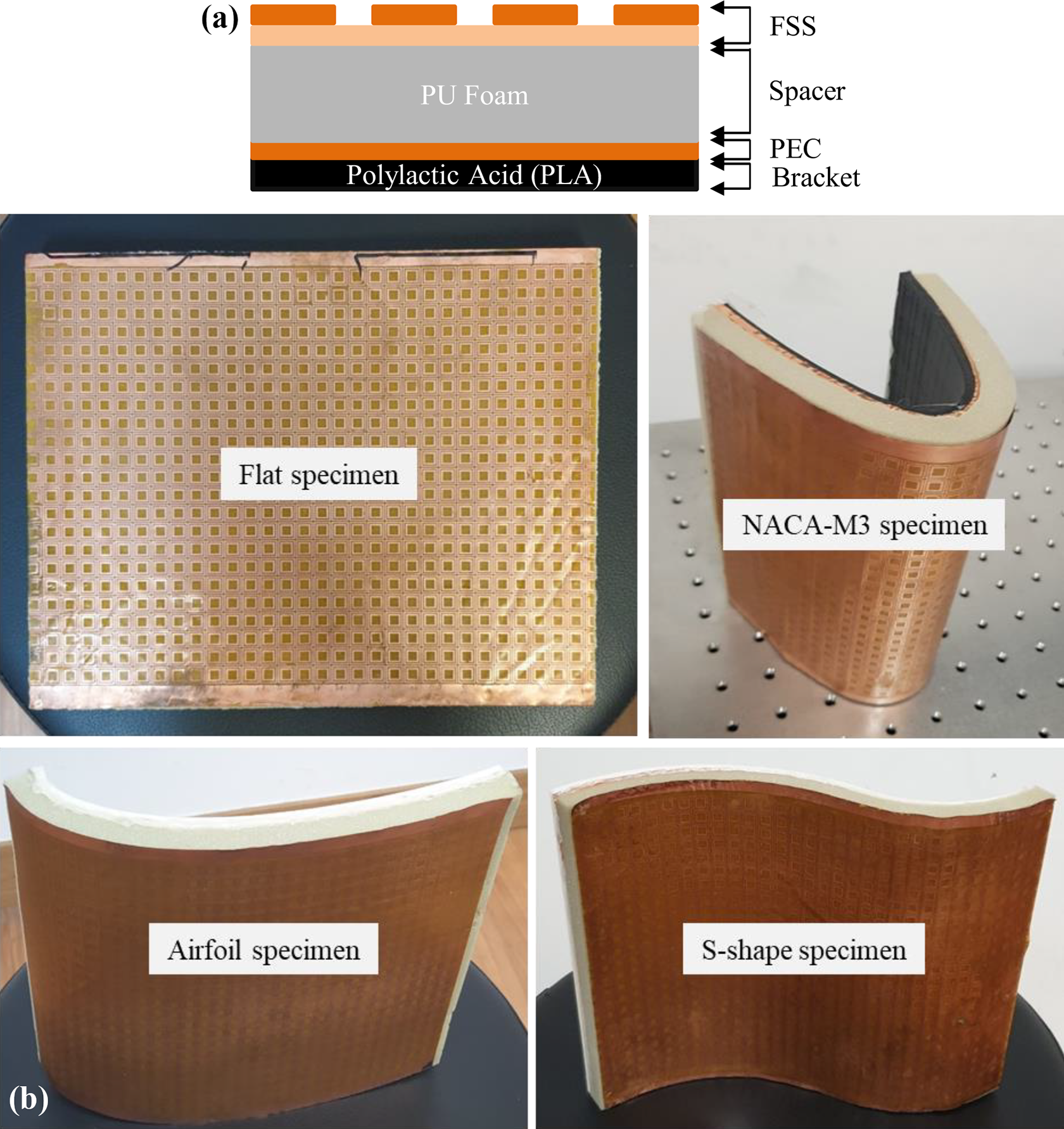
FSS sheet specimens: (a) cross section of RAS specimen and (b) fabricated specimens. FSS: frequency selective surface; RAS: radar absorbing structure.

Results and discussion

Flat RAS specimen

A flat RAS specimen (width: 250 mm, height: 200 mm, thickness: 12 mm) shown in Figure 7(b) was scanned to validate the performance of the six-axis RSFM setup. The inspection was performed using a scan area of width: 300 mm, height: 210 mm, and interval: 10 mm with 201 sweep points in the designed X-band frequency range. The spectrogram in Figure 8(a) clearly shows the specimen edge-affected results, mounting bracket effect, and results reflecting the background. The EM wave spot diameter at the focal length of the antenna is 60 mm, which is also noticeable from the edge-affected results. Nothing affects the results in the effective region (shown in the green box) since the specimen has a perfect rectangular flat surface.

Figure 8.

Flat RAS specimen (width: 250 mm, height: 200 mm, thickness: 12 mm) (a) S ₁₁ spectrogram at 8.2 GHz and (b) pointwise results from the region (A, B, C). RAS: radar absorbing structure.

The results obtained from the specimen (encircled in a red box) clearly show the specimen’s shape and its correct width and height. The return loss signal gradually decreases at the edges since the percentage of the beam overlapping the specimen gradually decreases as the scan moves beyond the edges of the specimen. The effect of the fixture bracket can also be seen at the side bottom of the spectrogram. The specimen showed quite uniform results throughout the effective area of the specimen. The effective area is divided into three different regions to study the effect of curvature on resonant frequency return loss, as the same specimen FSS sheet is used in the double curvature specimen. From Figure 8(b), the average pointwise results in region A have a resonant frequency of 10.34 GHz with a return loss value of −9.063 dB; region B has a resonant frequency of 10.32 GHz and return loss value of −9.206 dB. In comparison, region C has a resonant frequency of 10.38 GHz with a return loss value of −7.299 dB. The resonant frequency of each region is very similar (on average 10.35 GHz). Still, there is a slight difference between the return loss values, especially in region C, which has a lower value than A and B. Framewise results for all 201 sweep frequency points within the X-band range are also included in the supplementary data accompanying this writing.

Leading-edge RAS specimen NACA-M3

A leading-edge specimen NACA-M3 (arc length: 240 mm, height: 200 mm, thickness: 12 mm), as shown in Figure 7(b), is used for evaluation using a six-axis RSFM. The scan area of inspection was 250 mm x 210 mm, and interval of 10 mm with 201 sweep points in the designed X-band frequency range. The specimen has a variable curvature, yet the geometry is symmetrical. The scan results clearly show that the effective area is only affected by the radius of curvature (ROC), as the results are symmetrical, like the specimen geometry. A video file showing the scan result has also been included in the supplementary data accompanying this writing. Figure 9(a) shows the frame at 8.2 GHz; it is evident from the spectrogram that RAS does not show any absorption at this frequency.

Figure 9.

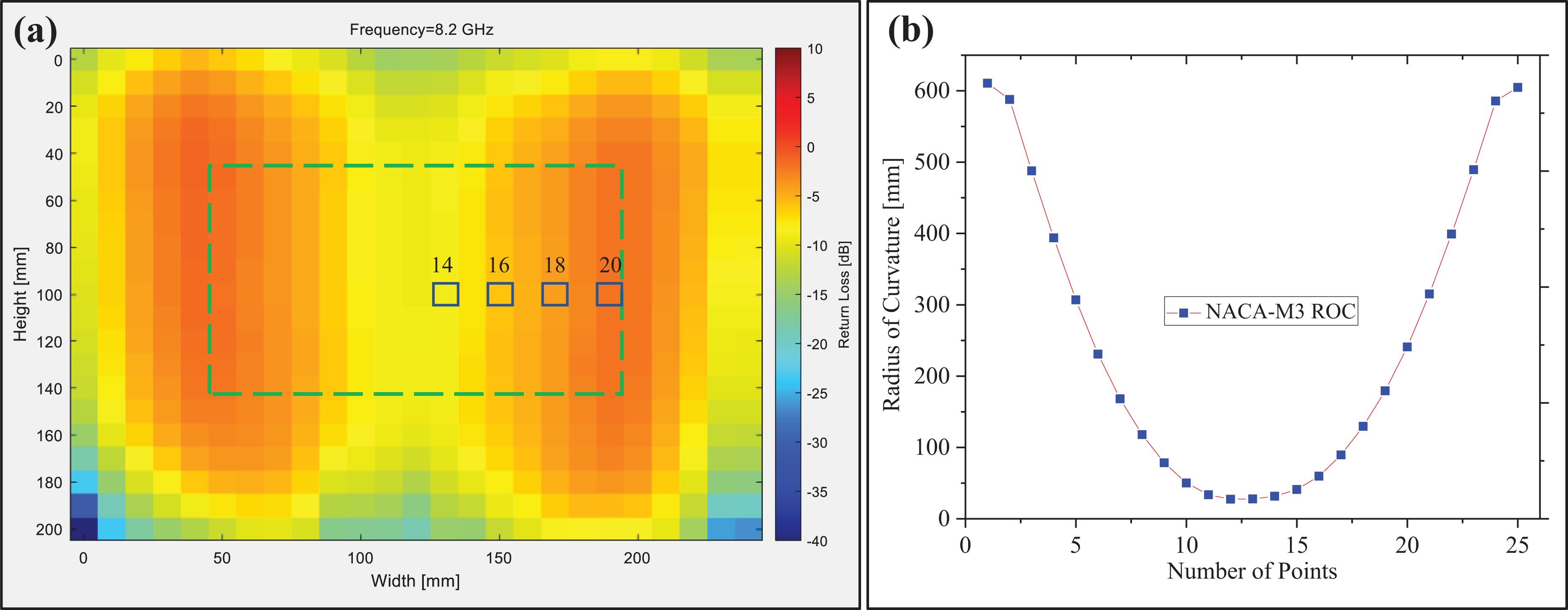
NACA-M3 specimen (a) six-axis RSFM scan results S ₁₁ spectrogram at 8.2 GHz and (b) radius of curvature. RSFM: robotic scanning free-space measurement.

Additionally, the result also shows the edge effect and mounting bracket effect outside the effective area of the scan. From the ROC graph shown in Figure 9(b) and the results, we could say that the return loss value decreases with the increase in ROC. Alternatively, the higher the curvature is, the higher the return loss.

The results obtained for the NACA-M3 specimen with six-axis RSFM were compared with those obtained by a conventional three-axis SFM with horizontal and vertical axes transitions on the specimen projection and rotation about the vertical axis. The frequency responses from different parts of the effective scan area, marked on the spectrogram, are used for pointwise result comparison. The scan parameters calculated by the algorithm are the ROC, incident angle, and scan point SOD from the antenna, as shown in Table 1. The pointwise results for the three-axis SFM are shown in Figure 10(b). The results show that the return loss decreases with the increase in the ROC. Overall, the specimen does not show good RAS performance, and the highest absorption occurs between 10 GHz and 10.5 GHz. The six-axis RSFM pointwise results are shown in Figure 10(a). In the six-axis RSFM results, the specimen shows the same behavior regarding the curvature effect but better absorption than the three-axis SFM between 10 GHz and 10.5 GHz frequency. The SOD effect caused the lesser absorption for the resonant frequency in the three-axis SFM results. From Table 1, we see that the three-axis SFM does not inspect the specimen at the calibrated focal length of 430 mm. These results indicate that the six-axis RSFM system maintains a target point on the calibrated focal length of the antenna while measuring and thus gives highly accurate results for complex curvature specimens.

Table 1.

NACA-M3 incident angles, the radius of curvature, and standoff distance for six-axis RSFM and three-axis SFM.

X (mm)	Y (mm)	Point	Incident angle (°)	Radius of curvature (mm)	Standoff distance (mm)
					Six-axis RSFM	Three-axis SFM
130	100	14	0	29.93	430	410.52
150	100	16	0	51.99	430	413.4
170	100	18	0	119.65	430	413.68
190	100	20	0	341.85	430	412.7

RSFM: robotic scanning free-space measurement; SFM: scanning free-space measurement.

Figure 10.

Pointwise scan results for NACA-M3: (a) six-axis RSFM and (b) three-axis SFM. RSFM: robotic scanning free-space measurement; SFM: scanning free-space measurement.

Airfoil shape RAS specimen

The developed six-axis RSFM system was also verified with an airfoil specimen having variable curvature and nonsymmetrical geometry, as shown in Figure 7(b). A specimen coordinate graph and ROC graph are shown in Figure 11. The scan results are comparable to the specimen ROC graph. The reflection loss is higher for smaller ROCs and vice versa. Figure 12(a) shows the frame at 8.2 GHz; it is evident from the spectrogram that the specimen does not show any absorption at this frequency. A video file showing the scan result has also been included in the supplementary data accompanying this writing.

Figure 11.

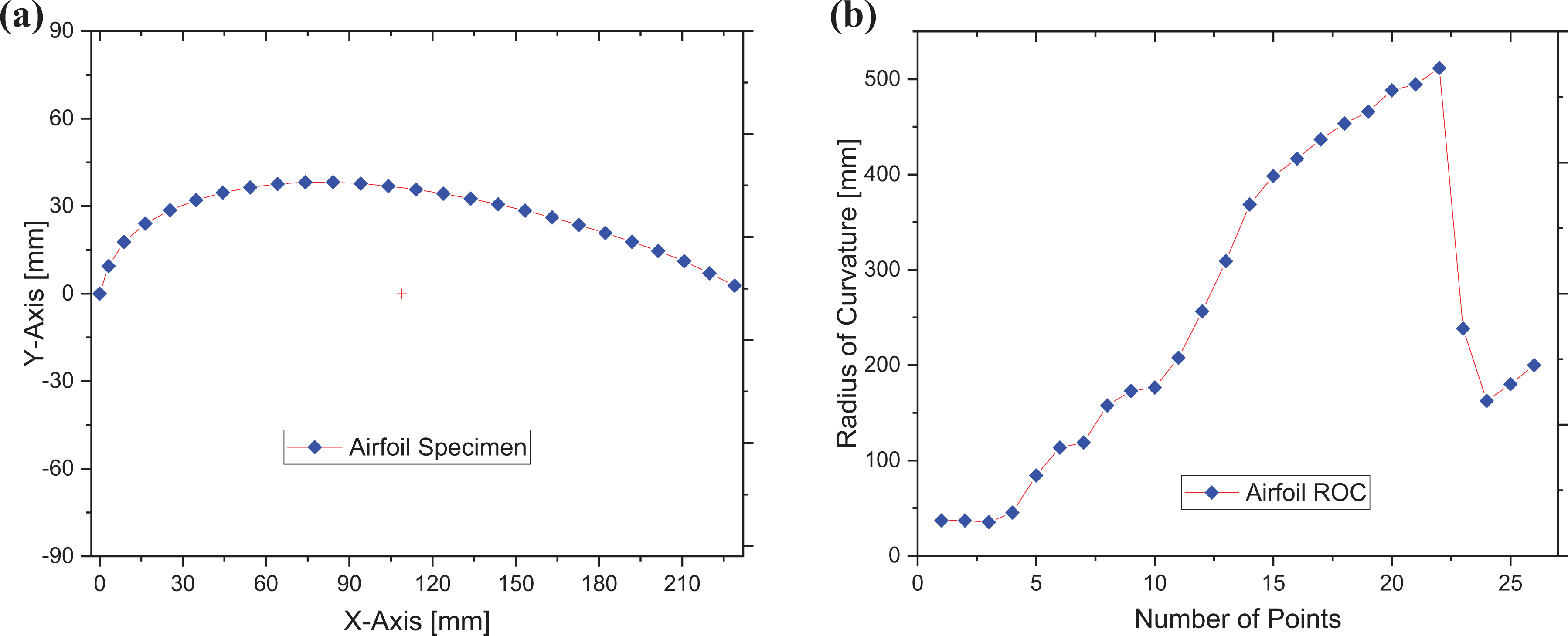
Airfoil specimen: (a) XY coordinate and (b) radius of curvature.

Figure 12.

Six-axis RSFM scan results of airfoil RAS specimen: (a) S ₁₁ spectrogram at 8.2 GHz and (b) pointwise results. RSFM: robotic scanning free-space measurement.

Additionally, the result also shows the behavior at the boundaries. A pointwise response from the affective area for four different points’ details given in Table 2 is shown in Figure 12(b). The ROC is high, and the SOD is 430 mm, like the calibrated focal length in the effective area; thus, the return loss results show similar reflection loss. The pointwise results clearly show that the robot’s extra axis eliminates the SOD effect. The highest absorption frequency for this specimen is approximately 10.8 GHz, where the reflection loss is about −14 dB.

Table 2.

Six-axis RSFM incident angles, the radius of curvature, and standoff distance at four different points of the airfoil specimen.

X (mm)	Y (mm)	Point	Incident angle (°)	Radius of curvature (mm)	Standoff distance (mm)
120	100	13	0	368.607	430
140	100	15	0	416.544	430
160	100	17	0	453.468	430
180	100	19	0	488.237	430

RSFM: robotic scanning free-space measurement.

S-shaped double curvature RAS specimen

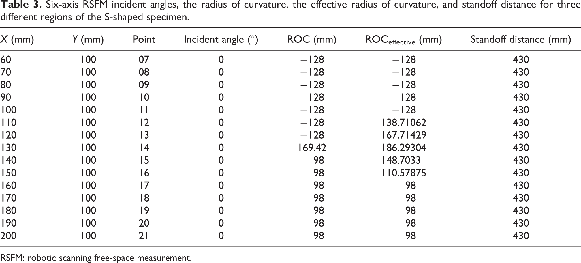
A double curvature S-shaped RAS specimen (arc length: 250 mm, height: 200 mm, thickness: 12 mm) was made using the same FSS sheet used in the above flat specimen. The actual double curvature RAS specimen is shown above in Figure 7(b). It was a bit difficult to make a perfect S-shaped specimen from the used material FSS sheet and the soft PU foam spacer. An extremely accurate specimen adhering exactly to the bracket shape is only possible when made from a rigid material using an autoclave or some other machining process. Therefore, an optimal S-shaped specimen was manufactured just to evaluate the six-axis RSFM system. The specimen has many localized anomalies due to the excessive amount of adhesive spray, as the FSS sheet is utilized twice. In the regions where the curvature is constant, localized anomalies could be removed using averaging results.

The scanning measurement was performed using a scan area of a width of 260 mm, a height of 210 mm, and an interval of 10 mm with 201 sweep points in the designed X-band frequency range. A framewise spectrogram for frequency 8.2 GHz is shown in Figure 13(a). This is a double curvature specimen; it has a different ROC in each region. The ROC of region A is −128 mm and that of region B is 98 mm, while there is a transition line in between, as shown in Figure 13(b). The spectrogram results clearly show a difference in return loss of each region. The effect of the mounting bracket is also highlighted. When the curvature radius is −128 mm, the average absorption frequency is 10.07 GHz, and the minimum reflection loss is −12.13 dB, as shown in Figure 13(c). For the 98 mm curvature radius, the average absorption frequency is 10.4 GHz, and the minimum reflection loss is approximately −16.15 dB, as shown in Figure 13(d). The difference in the reflection loss values between regions A and C is due to the ROC difference. Around the transition line, the absorption frequency and the reflection loss distribution of the specimen are not uniform because of the spot size overlapping effect.

Figure 13.

Robotic SFM scan results of the S-shaped (a) S ₁₁ spectrogram at 8.2 GHz, (b) radius of curvature graph, (c) region A pointwise results, and (d) region C pointwise results. SFM: robotic scanning free-space measurement.

From the ROC graph, we can see a single point of transition, but the transition region results show an almost 50 mm width. This is because of the spot size overlapping effect. The spot size diameter of the antenna is 60 mm. When measuring variable curvature specimens, the result is affected by all the curvatures that come within the EM wave spot size. In addition, a focused EM wave has a Gaussian power distribution, as shown in Figure 14. Therefore, all the curvatures and the distribution of EM waves must be considered when calculating the effective ROC. The effective ROC can be found from Gaussian averaging of the ROC within the spot size area using the formula below

${\text{ROC}}_{\text{effective}}=\frac{1}{273}\left({\text{ROC}}_{11}\text{* }{W}_{11}+{\text{ROC}}_{12}\text{* }{W}_{12}+\cdots +{\text{ROC}}_{55}\text{* }{W}_{55}\right)$

1

where ROC_effective is the effective ROC, W is the weight ratio of the Gaussian matrix, and the subscripts represent matrix position.

In the above equation, W is the weight ratio of the Gaussian matrix as shown in Figure 14. Each segment of the focused EM wave Gaussian matrix is equal to the scan interval.

Figure 14.

Gaussian distribution and matrix of the electromagnetic wave. ¹⁸

The absolute values of the effective ROC of the S-shaped specimen are shown in Figure 15(b). The actual values of the effective ROC for all three regions can be seen in Table 3. These values show that the transition region will have at least 50 mm width and different return loss values, as seen from the pointwise results shown in Figure 15(a).

Figure 15.

S-shaped RAS specimen: (a) transition region pointwise results and (b) effective ROC curve. RAS: radar absorbing structure; ROC: radius of curvature.

Table 3.

Six-axis RSFM incident angles, the radius of curvature, the effective radius of curvature, and standoff distance for three different regions of the S-shaped specimen.

X (mm)	Y (mm)	Point	Incident angle (°)	ROC (mm)	ROCeffective (mm)	Standoff distance (mm)
60	100	07	0	−128	−128	430
70	100	08	0	−128	−128	430
80	100	09	0	−128	−128	430
90	100	10	0	−128	−128	430
100	100	11	0	−128	−128	430
110	100	12	0	−128	138.71062	430
120	100	13	0	−128	167.71429	430
130	100	14	0	169.42	186.29304	430
140	100	15	0	98	148.7033	430
150	100	16	0	98	110.57875	430
160	100	17	0	98	98	430
170	100	18	0	98	98	430
180	100	19	0	98	98	430
190	100	20	0	98	98	430
200	100	21	0	98	98	430

RSFM: robotic scanning free-space measurement.

Curvature effect on the resonant frequency

The six-axis RSFM scans a double curvature specimen at zero incident angle and calibrated focal length of the antenna. Therefore, the results are only affected by curvature, as shown in Table 3. The curvature effect was removed from the results using the curvature compensation method developed by Son et al. ²⁴ From Figure 16, we can see that the results revert to their original return loss values obtained for the flat specimen above. However, the resonant frequency return loss values show some difference from the flat specimen resonant frequency values. This means that the curvature affects the resonance frequency values, which cannot be compensated using PEC curvature compensation. In region A, where the curvature is negative, the S-shaped specimen has a return loss value of −8.456 dB, while the flat specimen shows a return loss of −9.063 dB. Therefore, overall, the negative curvature reduces the return loss value of the resonant frequency.

Figure 16.

S-shaped RAS specimen curvature compensated pointwise results: (a) region A and (b) region B. RAS: radar absorbing structure.

Similarly, in region B, where the curvature is positive, the S-shaped specimen has a return loss value of −10.2 dB, while the flat specimen shows a return loss of −7.299 dB. Therefore, overall, a positive curvature increases the return loss value of the resonant frequency. A similar result was obtained by Son et al. ²⁴ for S-shaped specimens using two-axis SFM. To conclude, the negative curvature reduces the resonant frequency return loss due to the compression of the outer surface of the specimen, as shown by region A, and the positive curvature increases the resonant frequency return loss due to the expansion of the specimen, as shown by region C. These results show that six-axis RSFM has been applied to EM evaluation as well as non-destructive testing by Lee et al. ²⁵ of curvature specimens.

Conclusion

This article presents a six-axis RSFM system for the EM evaluation of highly curved 3D stealth structures. This system enables accurate and efficient scanning of the complex RASs for return loss evaluation. With the help of the six-axis robot manipulator, the system moves the specimen in front of the radiating horn antenna, which enables the normal incidence scan of the specimen at the calibrated focal length of the antenna, so we have a uniform spot size of incident EM waves. The six-axis RSFM was verified with four different shape RASs, namely flat, NACA-M3, airfoil, and S-shaped double curvature specimens. Highly accurate scan results, with zero-degree incident scan and calibrated focal length (430 mm) of the antenna, were obtained for all four specimens. Compared to three-axis SFM the six-axis RSFM resonance frequency EM waves show high absorption for the NACA-M3 RAS specimen, as the three-axis SFM cannot scan at the calibrated focal point of the antenna.

A user-friendly GUI software controls the whole system and visualizes real-time results. This software stores the results in a 3D array that can be visualized framewise and pointwise. The simulation of the system is performed in RobotStudio using a virtual robot controller. The specimen coordinates and RPY angles are then automatically extracted in RobotStudio. Each scan point extracted coordinates are then transformed into robot manipulator wrist coordinates by a robotic scanning algorithm to make a scan path trajectory. Finally, an effective ROC curve for the variable curvature specimen was formalized using the Gaussian distribution matrix of EM wave spot size. Based on effective ROC values, it was easy to study the results of the transition region of the S-shaped specimen.

In conclusion, a six-axis RSFM system can be used for the accurate return loss properties evaluation of arbitrarily shaped stealth structures. In the future, this system can be upgraded to the two-port system which will enable other EM properties evaluation in addition to return loss. For non-robotic users, making the simulation and extracting the target scan points from a CAD model of specimen in RobotStudio could be a difficult task. Similarly, manual conversion of target points RPY Euler angles to quartering angles for robot manipulator move command to make a scan trajectory is also an issue. Both these problems can be solved if an algorithm of the target point extraction and automatic conversion to robot command is implemented in GUI software.