Sage Journals: Discover world-class research

Abstract

Recently, the learning-based LiDAR odometry has obtained robust estimation results in the field of mobile robot localization, but most of them are constructed based on the idea of supervised learning. In the network training stage, these supervised learning-based methods rely heavily on real pose labels, which is defective in practical applications. Different from these methods, a novel self-supervised LiDAR odometry, namely SSLO, is proposed in this article. The proposed SSLO only uses unlabeled point cloud data to train the three-view pose network to complete the robot localization task. Specifically, first, due to the sparseness and disorder of the original LiDAR point cloud, it is difficult to use deep convolutional neural networks for feature extraction. In this article, the spherical projection of the point cloud is used to convert the original point cloud into a regular vertex map. Then the vertex map obtained by the projection is used as the input of the neural network. Second, in the network training phase, SSLO uses multiple geometric losses for different situations of matching point clouds and introduces uncertainty weights when calculating the losses to reduce the interference of noise or moving objects in the scene. Last but not least, the proposed method is not only used in the simulation experiments based on the KITTI dataset and Apollo-SouthBay dataset but also applied to a real-world wheeled robot SLAM task. Extensive experimental results show that the proposed method has good performance in different environments.

Keywords

Point cloud SLAM self-supervised learning spherical projection vertex map

Introduction

Estimating the self-motion of mobile robots is an important prerequisite for robotic autonomous exploration. With the development of autonomous driving, the real-time locating and path planning of mobile robots are receiving increasing attention and research. In outdoor environments, people can usually apply a global positioning system (GPS) to locate the robot. However, in some special environments, such as long tunnels, dense high-rise buildings, and forests, GPS cannot continuously and stably complete reliable positioning tasks. In this case, the robot needs to use its onboard sensors to estimate its pose. LiDAR has high resolution and a strong interference ability and is not affected by light, and with the accumulation and innovation of optical technology, the LiDAR size, weight, and price are decreasing. Another important advantage of LiDAR is to directly obtain the depth of the object in the environment, which overcomes the monocular camera scale uncertainty, so using LiDAR to complete robot motion estimation has become increasingly popular.

Among the available methods of using LiDAR for estimating the robot position, the most common method is based on iterative matching. The iterative closest point (ICP) and its variant¹ solve the best relative translation and rotation between two poses by minimizing the distance of the closest point in the continuous LiDAR scans. However, the ICP method is sensitive to the initial value. A good matching result requires a relatively accurate initial estimate. At the same time, to maintain the real-time operation of the system, the original point cloud data need to be down-sampled when performing ICP, which can destroy the original physical structure of objects, and result in points on objects in one frame missing their spatial correspondence in the next frame. Another approach is the feature-based method.² Feature-based methods are less sensitive to the scanning quality and more powerful; however, they are generally more computationally expensive. Notably, they are sensitive to dynamic objects in the scene. These shortcomings hinder the application of feature-based matching methods to odometries.

Recently, visual odometry (VO)^3

–6 based on deep learning has achieved superior results over classical VO in some three-dimensional tasks. These methods provide new solutions for robot pose estimation tasks using point cloud data. The point cloud data captured from distance sensors are sparse and irregular, and it is difficult to directly perform a 6-DOF pose regression using traditional convolutional neural networks (CNNs). To compute the pose of the robot, such as with deep VO, Li et al.⁷ projected the original 3D point clouds into 2D images and performed pose estimation with a neural network. Li et al.⁸ take monocular images and point cloud projection images as the input and design an end-to-end odometry network to fuse two kinds of input data to generate pose estimation in a learning manner. Furthermore, most of the proposed deep LiDAR odometries are constructed in supervised learning ways, and the accuracy of these methods relies heavily on large-scale annotated training data, which is not always feasible in practice because large-scale labeling is quite expensive, which limits the scope of application of such methods. How to use unlabeled data to design depth LiDAR odometry is still a problem that needs to be solved urgently.

To avoid the time-consuming labeling process, we propose a novel self-supervised learning odometry. This method only needs unlabeled data to complete the learning of neural network and the positioning task of robot. The method proposed in this article takes the vertex map obtained by point cloud spherical projection as the input, which can preserve the spatial structure of objects in the environment as much as possible and alleviate the problem that disordered and sparse point clouds have difficulty using neural networks for feature extraction. Because the premise that a SLAM system can run is that the observed environment is static and there are no dynamic objects. If there are dynamic objects in the scene, the SLAM assumptions will be broken, which will lead to poor positioning accuracy or even failure of the SLAM algorithm. However, in actual applications, dynamic objects generally exist in the environment. So, it is necessary to minimize the impact of dynamic objects when constructing the SLAM system, which helps to improve the positioning accuracy of the system. To reduce the interference of noise and dynamic objects, weighted point-to-point, weighted point-to-plane, and weighted plane-to-plane losses are used in the training phase to constrain different point cloud correspondences in continuous scanning frames. It forces neural network to pay more attention to the static features of the environment and ignore the dynamic and unstable features. Figure 1 shows the KITTI sequence 07 trajectory map estimated after network training without the ground truth pose. The point cloud is colored according to the time stamp, and the color transitions from blue to green as time increases. The figure shows that the method in this article successfully captures the motion trajectory of the mobile robot.

Figure 1.

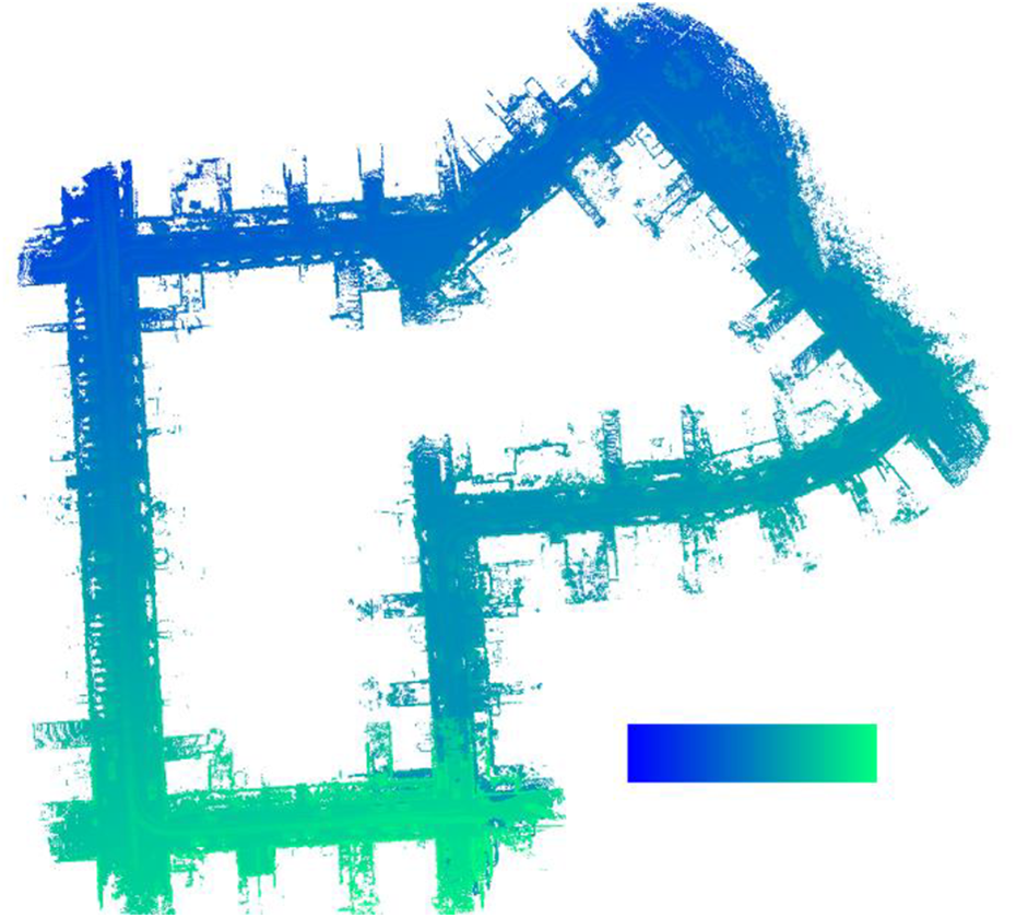
Point cloud map estimated using LiDAR odometry.

The main contributions of the method in this article are as follows:

This article proposes a LiDAR odometry framework based on self-supervised learning, which takes the vertex map generated by the point cloud as the input to predict the ego-motion of LiDAR.

A simple and fast method to calculate the point weights is proposed, which is combined with the self-supervised loss function to better address the problems of noise and dynamic objects in the environment.

The method in this article is experimentally verified on the KITTI dataset, Apollo-SouthBay dataset, and real-world environments and compared with the existing methods, which proves the effectiveness of the proposed method.

The remainder of this article is as follows. Traditional and learning-based LiDAR odometry works are reviewed in the second section. In the third section, the architecture and loss function of the proposed self-supervised deep LiDAR odometry are elaborated. Experimental results and comparisons with other methods are detailed in the fourth section. Finally, the conclusions and future work are discussed in the fifth section.

Related work

LiDAR-based pose estimation algorithms can be roughly divided into two categories. One category is model-based methods, such as ICP and its various variants. ICP aligns the scan and model point clouds in an iterative two-step process. In the first step, the algorithm establishes the correspondence between the two point cloud scans. The second step calculates a transformation to reduce the distance between all corresponding points and repeats these two steps with the transformed scan until a certain optimization criterion is reached. Model-based methods have been proposed in the extensive literature. LiDAR odometry and mapping (LOAM)⁹ performs point-to-edge and point-to-plane scanning matching and achieves low drift and low computational complexity of the odometry through parallel high-frequency and low-frequency modules. LOAM is one of the best frameworks. Many works have been developed based on LOAM. LEGO-LOAM¹⁰ proposes a lightweight and ground-optimized SLAM algorithm, which achieves similar accuracy with reduced computational cost. Intensity-SLAM¹¹ is a complete SLAM framework that combines geometric features and strength information features. Combining intensity information helps to identify the same features on multiple frames. This method uses the scan-to-global map matching method to calculate the optimal pose by minimizing geometric residuals and intensity residuals. LiTAMIN¹² uses the Frobenius norm and regularized covariance matrix to normalize the cost function to improve the computational efficiency of ICP. M-LOAM¹³ is a SLAM framework that combines multiple LiDARs. It estimates the pose through online calibration optimization and convergence recognition. The experimental results show that it has a better positioning accuracy than a single LiDAR system. However, the algorithm based on LOAM needs to down-sample the point cloud data during the execution stage, which cannot accurately represent the underlying local surface structure. SUMA¹⁴ proposes a dense LiDAR-based SLAM method to construct a Surfel-based map and estimates the transformation of the robot pose by using the projection data association between the current scan and the rendered model view from the Surfel map. However, the sparse point cloud is a challenge. Li et al.¹⁵ proposed a mobile robot system that combines LIDAR, IMU, and GNSS data. The system performed point cloud registration on GPU, which improves computing efficiency. In addition, a hierarchical optimization structure was proposed to improve the mapping quality. Zheng and Zhu¹⁶ used a bird’s-eye view that effectively retains the neighborhood relationship of ground surface points nearly parallel to laser beams. This method obtained better results than SUMA. Jiang et al.¹⁷ took LiDAR and inertial measurement unit (IMU) data as the input and used the rank Kalman filter to estimate the robot’s pose, which improved the accuracy and robustness of the robot’s indoor positioning. Demim et al.¹⁸ proposed the SVSF-SLAM algorithm, which has better robustness and accuracy. Compared with EKF-SLAM, SVSF-SLAM has the advantages of low computational complexity, high estimation accuracy, and robustness. Mosbah et al.¹⁹ described a SLAM method based on second-order smooth variable structure filter embedded in a mobile robot. Compared with the competitors, Mosbah’s method obtained higher positioning accuracy and robustness.

Compared with model-based LiDAR odometry, the learning-based LiDAR odometry method is not perfect. As a technical solution to the robot navigation problem, it is attracting increasing research interests and shows the great potential of this approach. StickyPillars²⁰ is a fast and accurate point cloud registration method based on a graph convolutional network, and the registration result is better than the feature registration method based on ICP. SLOAM²¹ uses semantic segmentation to detect tree trunks and the ground, separately models them, and proposes a pose optimization method based on semantic features, which achieves better results than traditional methods in a forest environment. Unlike SLOAM, Yue et al.²² proposed a semantic SLAM system that integrated camera and LiDAR. The system obtains semantic information from image data and combines the semantic information with point clouds to complete the collaborative semantic mapping. S-ALOAM²³ integrates semantic information into the LOAM pipeline and uses point-by-point semantic labels for optimization in the dynamic point elimination stage, feature selection stage, and corresponding point searching stage. The experimental results demonstrate that this method outperforms the state-of-the-art SLAM methods. Dmlo²⁴ explicitly implements geometric constraints in the framework and decomposes pose estimation into two parts: a learning-based matching network to provide accurate correspondence for two scans and rigid transformation estimation using singular value decomposition, which yields comparable or better results to conventional LiDAR odometry methods. As an improved version of SUMA, SUMA++²⁵ combines semantic information to constrain the projection match and thus can reliably filter moving targets in the scene and achieve the most advanced performance. These methods are all successful applications of deep learning in LiDAR odometry. However, they only use deep learning for intermediate feature extraction, and odometry estimation is still obtained through geometric transformation. Lo-net is the first learning-based end-to-end LiDAR odometry with continuous point cloud scanning as the input to directly output the relative transformation while designing a mask network to compensate for dynamic objects in the scene; thus, it eventually yields an accuracy similar to that of LOAM. Deeppco²⁶ designed two parallel subnetworks to estimate translation and rotation and achieved a performance comparable to traditional methods. Both Lo-net and Deeppco train the framework in a supervised learning manner, which limits their application scenarios.

In reality, obtaining the true value of the pose often takes considerable energy. How to fully use all point cloud data to train the pose network is a challenging and meaningful research. Cho et al.²⁷ proposed the first LiDAR odometry implemented in an unsupervised manner, introducing an uncertainty-aware loss with geometric confidence that successfully captures the relative motion of large-scale trajectories. Nubert et al.²⁸ proposed a self-supervised LiDAR odometry method using point-to-plane and plane-to-plane geometric loss and used Kd-Tree in the corresponding point searching strategy to search for the relationship between the source domain and the target domain in a 3D space without additional visual field loss. The experimental results show that the proposed method achieves similar accuracy to LOAM. Similar to the works of Cho and Nubert, this article is dedicated to the design of a self-supervised deep LiDAR odometry to achieve accurate pose estimation by fully utilizing all available LiDAR data while avoiding the effects of outliers and motion targets using multiple geometric consistency-weighted losses in different scenarios.

Proposed approach

In this section, the proposed method is described in detail. First, the pose estimation problem is modeled; second, this article uses the same projection function $\prod : ℝ^{3} \mapsto ℝ^{2}$ as Chen et al.²⁹ to generate a vertex map $V : ℝ^{2} \mapsto ℝ^{3}$ and map the two-dimensional image coordinates ${(u, v)}^{T} \in ℝ^{2}$ to points ${(x, y, z)}^{T} \in ℝ^{3}$ . Then, the normal vector corresponding to each vertex is calculated offline according to the vertex map generated by the projection, and the generated normal map and vertex map are used as the input for network training. Then, the proposed self-supervised network structure is explained in detail. Finally, various self-supervised geometric losses in this article are introduced.

Problem statement

The problem of estimating the robot pose transformation $T_{t - 1, t} \in S E (3)$ , which projects the robot pose at time t to time $t - 1$ , from adjacent continuous point cloud scans $S_{t - 1} \in ℝ^{n_{t - 1} \times 3}$ and $S_{t} \in ℝ^{n_{t} \times 3}$ with noise, can be solved by probabilistic modeling using the following equation

p (T_{t - 1, t} | S_{t - 1, t}, S_{t})

The key to modeling is to solve the probability density function p. The traditional method converts the probability problem into a least square problem and uses an iterative method to solve it. This article uses a deep neural network to model the pose estimation problem, that is, $T_{t - 1, t} = f (θ, S_{t - 1}, S_{t})$ , where $f (•)$ is the network model, and $θ$ is the trainable parameter of the neural network. After solving $θ$ through the training of the network, the transformation matrix between different scans can be estimated according to the input scans $S_{t - 1}$ and S_t . The specific odometry network is described in detail in section “Network architecture.”

Input projection

The point cloud obtained from the LiDAR is usually represented by the Cartesian coordinate system. To convert the original sparse and irregular point cloud into a data format that can be conveniently processed by the CNN, this article uses efficient and dense point cloud spherical projection to project the point cloud data P into a regular vertex map $V : ℝ^{2} \mapsto ℝ^{3}$ . Each pixel of the vertex map stores the specific value (x, y, z) of the corresponded point cloud scan. If there are multiple 3D points projected on the same pixel coordinate, the one with the smallest distance among all 3D points projected on the pixel coordinate is selected as the pixel value. Each point $p_{i} = (x, y, z)$ is projected to the spherical coordinate system through the function $\prod : ℝ^{3} \mapsto ℝ^{2}$ and then projected to the 2D image coordinate system $(u, v) \in ℝ^{2}$ . The projection formula is as follows

(\begin{matrix} u \\ v \end{matrix}) = (\begin{matrix} \frac{1}{2} [1 - arctan (y, x) \cdot π^{- 1}] \cdot w \\ [1 - (arcsin (z \cdot r^{- 1}) + f_{up}) f^{- 1}] \cdot h \end{matrix})

where w and h are the width and height, respectively, of the vertex map V generated by the projection, $r = \sqrt{x^{2} + y^{2} + z^{2}}$ is the distance value of each point p, and $f = f_{up} + f_{down}$ is the vertical field of view of the sensor. Figure 2 is an example of the vertex map V obtained from the point cloud P obtained at time t through projection. The first row (a) is the disordered point cloud output by the LiDAR, and the second row (b) is the vertex map obtained by spherical projection. For the convenience of visualization, the vertex map is RGB color coded according to the distance of each pixel from the center of the LiDAR.

Figure 2.

Point cloud spherical projection. (a) Raw point clouds from LiDAR; (b) the corresponding vertex map.

Normal calculation

To strengthen the geometric consistency during the training phase, the normal map N comprising the normal vectors n_i corresponding to the vertices v_i in the vertex map V is used when calculating the self-supervised loss. Since the calculation of the normal vector requires additional time overhead and the participation of the normal vector is not required during the inference period, unlike Chao et al.²⁷, this article estimates the normal mapNcorresponding to the vertex map V offline before network training. Given a point v_i in the vertex map and k neighboring points $v_{i}^{j}, j = 1, 2, ..., k$ around the point, the neighboring points are selected according to the pixel distance closest to v_i in the vertex map V. The normal of a point can be calculated by the following formula

\underset{N (v_{i})}{argmin} {‖ {[w_{i}^{1} (v_{i}^{1} - v_{i}), \dots, w_{i}^{k} (v_{i}^{k} - v_{i})]}^{T} N (v_{i}) ‖}_{2}

w_{i}^{k} = e^{- {‖ v_{i}^{k} - v_{i} ‖}_{2}}

where ${[\cdot]}^{T}$ is a two-dimensional matrix, $N (v_{i})$ is a normalized vector, $v_{i}^{k}$ is the k nearest neighbor of v_i , and $w_{i}^{k}$ is a weight coefficient. For formula (3), this article uses the simple normal estimation method, as shown in Figure 3, and calculates normal vector n_i of each point v_i by calculating the weighted cross product of the four neighbors $S_{i}^{4}$ above, below, and to the left and right of n_i .

Figure 3.

Normal data encoding.

{\hat{n}}_{i} = \sum_{v_{i}^{j}, v_{i}^{k} \in S_{i}^{4}} (w_{i}^{j} (v_{i}^{j} - v_{i}) \times w_{i}^{k} (v_{i}^{k} - v_{i}))

N (v_{i}) = n_{i} = \frac{{\hat{n}}_{i}}{‖ {\hat{n}}_{i} ‖}

Network architecture

The proposed network consists of two parts: a feature extraction network (Feature Net) and a 6-DOF pose regression network (Pose Net). Feature Net encodes the input frame and extracts the features. Pose Net decodes the input feature vectors to estimate the relative motion between the input frames. During training, Kd-tree is used to find the target correspondence in the three-dimensional space; then, the geometric loss is calculated and back-propagated to the network. As shown in Figure 4, Feature Net consists of a convolutional layer, a maximum pooling layer followed by eight residual blocks and an adaptive average pooling layer. The input of Feature Net is the vertex maps obtained by the projection of the adjacent LiDAR point cloud scans, which goes through the last residual block to output feature maps with a size of $(N \times 512 \times \frac{H}{4} \times \frac{W}{32})$ , and subsequently adaptive global average pooling of the feature maps for each channel to obtain a fixed-dimensional eigenvector comprised of individual eigenvalues, and the subsequent eigenvector flows into the Pose Net. For Pose Net, two similarly structured three-layer fully connected networks are designed to estimate the relative pose transformation. The eigenvectors from Feature Net flow into the rotating head to estimate the relative rotation and output a quaternion q, and the translation head to estimate the relative displacement outputs a translation vector t. The vector [ $q, t$ ] is finally constructed as a transformation matrix that simultaneously represents translation and rotation. The architecture of the network is shown in Table 1.

Figure 4.

Schematic diagram of the proposed network.

Table 1.

Layers of the network architecture.

	Operator	Stride	Filters	Size	Output shape
Feature Net	Conv2D	(1,2)	64	(3,3)	64×H×W/2
	Max pool	(1,2)	64	(3,3)	64×H×W/4
	Resnet block	(1,1)	64	(3,3)	64×H×W/4
	Resnet block	(1,1)	64	(3,3)	64×H×W/4
	Resnet block	(2,2)	128	(3,3)	128×H/2×W/8
	Resnet block	(1,1)	128	(3,3)	128×H/2×W/8
	Resnet block	(1,2)	256	(3,3)	256×H/2×W/16
	Resnet block	(1,1)	256	(3,3)	256×H/2×W/16
	Resnet block	(2,2)	512	(3,3)	512×H/4×W/32
	Resnet block	(1,1)	512	(3,3)	512×H/4×W/32
	Adaptavg pool	–	512	–	512
Pose Net	Linear	–	128	–	128
	Linear	–	32	–	32
	Linear	–	4/3	–	4/3

Loss function

The design of the loss function significantly affects the stability and accuracy of the entire network. Cho et al.²⁷ used projection data associations to search for correspondence points, but the method was unstable. In this regard, the author increased the FOV loss to prevent divergence training away from the FOV state, thus enabling stable training of the whole network. Unlike the above losses, inspired by model-based approaches¹⁴ and similar to a previous study,²⁸ this article combines multiple weighted geometric losses to measure the difference between the target scan and the source scan mapped to the target space. Assuming that each sequence contains $2 n + 1$ scans, this article defines the input vertex and normal map sequence by ${V_{t - n}, \dots, V_{t - 1}, V_{t}, V_{t + 1}, \dots, V_{t + n}}$ and ${N_{t - n}, \dots, N_{t - 1}, N_{t}, N_{t + 1}, \dots, N_{t + n}}$ , frames V_t and N_t are target scans, and the remaining scans are source scans defined by V_s and N_s , $s \in {t - n, \dots, t + n}, s \neq t$ . SSLO predicts the relative pose transformation $T_{s, t}$ of each target and source pair.

For a point v_s in the source scan V_s , this article directly establishes a KD-Tree in three-dimensional space to find its corresponding point in the target scan. As shown in Figure 4, the points v_s and n_s in the source domains V_s and N_s are projected to the target domain according to the transformation matrix T estimated by Pose Net to obtain ${\hat{v}}_{t}$ and ${\hat{n}}_{t}$ . Then, a three-dimensional KD-Tree is constructed in the target domains V_t and N_t to search for matching points v_t and n_t to establish matching pairs $({\hat{v}}_{t}, v_{t})$ and $({\hat{n}}_{t}, n_{t})$ . Finding the paired points in three-dimensional space does not require an additional field of view loss while allowing processing of the points near the sharp edges.²⁸ KD-Tree can output the Euclidean distance d_t of the paired points $({\hat{v}}_{t}, v_{t})$ while obtaining the matched pairs. However, the Euclidean distance of the paired points searched by KD-Tree will become larger due to the presence of noise and dynamic objects in the environment. Therefore, we calculate the corresponding weights according to the Euclidean distances of different pairing points. The larger the Euclidean distance, the smaller the weight of the pair of points. In this way, the points affected by noise and dynamic objects have less impact on the network during the training phase, thereby forcing the neural network to pay more attention to the characteristics of static objects in the scene. Therefore, the influence of noise and dynamic objects in the scene on odometry results can be reduced during the test phase. The following formula can be used to assign different weights to each point pair and subsequently construct a weighted geometric loss

w_{t} = e^{- d_{t}}

After searching for n_k matching pairs $({\hat{v}}_{t}, v_{t})$ from the source scan mapped to the target scan in the target domain V_t , this article calculates the residual of each matching pair and projects the residual on the target plane at that position as a point-to-plane loss, that is

ℒ_{p 2 n} = \frac{1}{n_{k}} \sum_{t = 1}^{n_{k}} w_{t} {‖ ({\hat{v}}_{t} - v_{t}) \cdot n_{t} ‖}_{2}^{2}

In extreme cases, the nearest point searching strategy will have an incorrect match. As shown in Figure 5, the green five-pointed star is the position of the LiDAR, the pink line and blue line are the two scans of the LiDAR at different positions, and the dashed ellipse represents the approximate plane where the black point is located. In this case, the closest points found by KD-Tree will have incorrect associations because their surface directions are inconsistent, so the plane-to-plane loss in the loss function will be increased to compare with the surface directions of the paired points to reduce the impact of these matches.

Figure 5.

Extreme situations may exist in the closest point search.

ℒ_{n 2 n} = \frac{1}{n_{k}} \sum_{t = 1}^{n_{k}} w_{t} {‖ {\hat{n}}_{t} - n_{t} ‖}_{2}^{2}

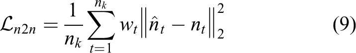
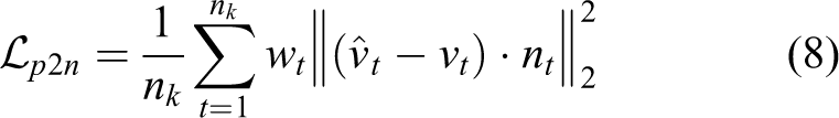
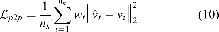
To make full use of all available points, this article calculates the point-to-point loss of each matching pair $({\hat{v}}_{t}, v_{t})$ for the points in the vertex map where the normal cannot be calculated.

ℒ_{p 2 p} = \frac{1}{n_{k}} \sum_{t = 1}^{n_{k}} w_{t} {‖ {\hat{v}}_{t} - v_{t} ‖}_{2}^{2}

In short, the self-supervised weighted geometric loss is

ℒ = ℒ_{p 2 n} + ℒ_{n 2 n} + ℒ_{p 2 p}

Experimental results

In this section, the implementation details and experimental results of SSLO are introduced. The system configuration of the network in the training phase is introduced in detail; then, the system performance is evaluated and compared with the existing self-motion estimation methods. The KITTI dataset, which is the one most widely used in autonomous driving, was used for benchmark testing. To evaluate the stability of the proposed network, the Apollo-SouthBay dataset was used to verify its multi-environmental adaptability.

Implementation details

The proposed network is constructed using the public PyTorch framework and trained using NVIDIA GTX1080Ti with the Adam solver in the training phase, where $β_{1} = 0.9, β_{2} = 0.999$ . We started the training with an initial learning rate of $10^{- 4}$ and subsequently applied a $50 %$ weight decay every 10 epochs. For the input LiDAR scan, we set $h = 64, w = 720$ to map the original point cloud into a $64 \times 720$ vertex map. In the training phase, the length of the input sequence is 3, the batch size is 4, and data shuffling was used to prevent overfitting.

Benchmark dataset

The KITTI odometry dataset is one of the most widely used datasets to evaluate odometry/SLAM algorithms. It consists of 22 independent suburban, highway, or urban driving sequences, and each sequence includes stereo grayscale and color camera images, point cloud data captured by LiDAR sensors, and calibration files. The point cloud data were collected with Velodyne HDL-64 at a sampling frequency of 10 Hz. Among these 22 sequences, only sequence 00-10 provides the ground truth pose obtained from the IMU/GPS fusion algorithm, while sequence 11-21 does not provide the ground truth pose for benchmarking.

The Apollo-SouthBay dataset contains six southern routes in San Francisco Bay area and covers various scenarios, including residential areas, urban areas, and highways. The dataset contains LiDAR scans, post-processed ground truth poses, and poses from the GNSS/IMU integration solution. Similar to the KITTI odometry dataset, this dataset uses Velodyne HDL-64 for point cloud data collection. The Apollo dataset sequence is longer than the KITTI sequence, the scenario is more complex, and it is more challenging to test the algorithm.

Experimental results

Evaluation on the KITTI dataset

The network was trained and evaluated on the KITTI dataset using the same training set/test set division strategy as other learning-based LiDAR odometries^27,28; that is, sequences 00-08 were used as the training set, and sequences 09 and 10 were used as the test set to verify the network performance. To quantitatively evaluate the accuracy of pose estimation, the evaluation criteria provided by the KITTI benchmark are used in this article to calculate the average translation $t_{rel} (%)$ and rotation $r_{rel} (° / 100 m)$ RMSEs of all possible subsequences between 100 m and 800 m. The specific results are shown in Table 2. The method in this article is also compared with other methods based on unsupervised learning, namely, SC-SfMLearner,³ DeepLO,²⁷ Li et al.,⁵ and DeLORA,²⁸ and with the current advanced model-based methods LOAM and SUMA. Since SUMA uses similar inputs and losses, the qualitative comparison guarantees the generality of the method, where the value of SUMA is taken from the results of the frame-by-frame estimation.¹⁴ From the experimental results of sequence 09, it can be seen that the average translation and rotation errors of the proposed method are significantly less than the existing end-to-end odometry methods. On sequence 10, the average translation error of this method is also less than other end-to-end learning-based methods, and the rotation error is slightly higher than that of Li’s method. However, the average translation error of this method is obviously lower than that of Li’s method. On the whole, the experimental results show that the method proposed in this article is better than other unsupervised learning odometries. However, the result is not as good as that of DeLORA+Map, which combines the DeLORA and LOAM mapping modules, because this method combines the LOAM low-frequency high-precision odometry module to further optimize the pose of the network output. Compared with SUMA, the method proposed in this article achieves better direction estimation results on sequence 10, which shows meaningful performance.

Table 2.

KITTI odometry evaluation: Comparison of the average translation and rotation errors of all possible lengths between 100 m and 800 m.

Methods		Sequence 09		Sequence 10
Methods		t _rel(%)	r _rel(°/100 m)	t _rel(%)	r _rel(°/100 m)
Model-based	LOAM	1.20	0.48	1.51	0.57
Model-based	SUMA	1.90	0.80	1.80	1.00
Learning-based	SC-SfMLearner	11.2	3.35	10.1	4.96
	Li et al	5.89	3.34	4.79	0.83
	DeepLO	4.87	1.95	5.02	1.83
	DeLORA	6.05	2.15	6.44	3.00
	DeLORA+Map	1.54	0.68	1.78	0.69
	Ours	2.00	0.88	2.27	0.92

Figure 6 shows the trajectory estimated by the method in this article on the KITTI dataset. From left to right and top to bottom are sequences 01, 07, 09, and 10 of KITTI. In this figure, the orange line is the ground truth value of the pose, and the blue line is the estimated value of the pose output by the network. The figure shows that the method in this article has a higher estimation accuracy for the rotation angle between adjacent frames, but the translation vector estimate has worse accuracy than the rotation angle estimation. SSLO has good estimation performance in different environments, especially in sequences that are not observed during training, but it can still maintain high accuracy.

Figure 6.

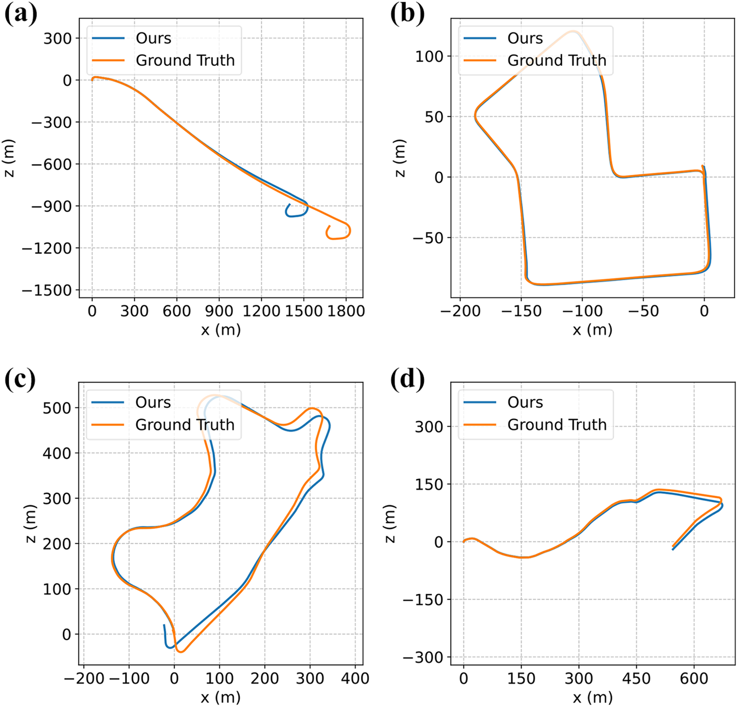
Trajectories of different sequences on the KITTI dataset. (a) Qualitative result on KITTI sequence 01; (b) qualitative result on KITTI sequence 07; (c) qualitative result on KITTI sequence 09; (d) qualitative result on KITTI sequence 10.

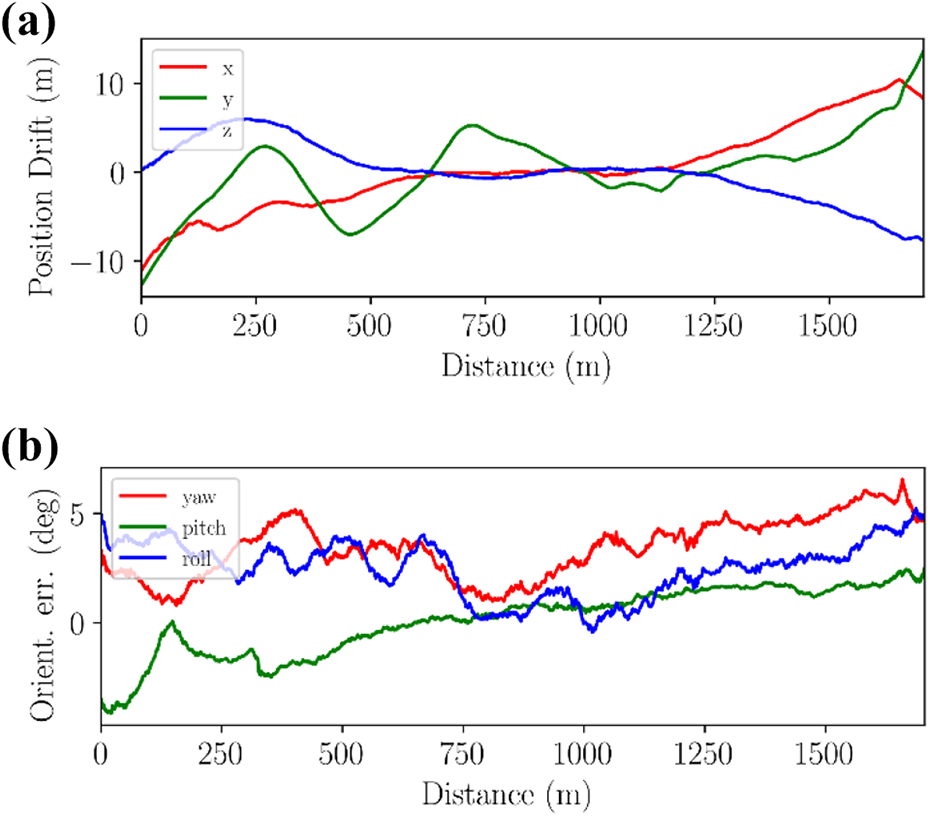
To carefully observe the performance of the proposed model, Figure 7 plots the error curve of the estimated pose on each degree of freedom on KITTI sequence 09 over time. Figure 7(a) shows the translation error along x, y, and z. Figure 7(b) shows the rotation error of the yaw angle, pitch angle, and roll angle. The maximum translation error in each coordinate axis direction is approximately $\pm 12 m$ , and the maximum error in the attitude angle direction is approximately $\pm 6^{\circ}$ .

Figure 7.

Translation and rotation errors. (a) Translation error of KITTI sequence 09; (b) rotation error of KITTI sequence 09. Evaluation on the Apollo-SouthBay dataset

Evaluation on the Apollo-SouthBay dataset

To verify the versatility of the method in this article, experiments were conducted on the San Jose Downtown sequence of the Apollo-SouthBay dataset and compared with the results of the pose estimation using the point-plane ICP algorithm in Open3d. The test trajectory is shown in Figure 8. The blue line in this figure is the method in this article, the purple line is ICP, and the orange line is the ground truth. When we evaluate the performance of the odometry, the translation and rotation errors obtained using the evaluation criteria provided by the KITTI benchmark are shown in Table 3. The comparison results show that the method in this article is better than traditional point-plane ICP. Point-plane ICP obtains very poor estimation results in a scene with many moving objects; in particular, the estimation of translation cannot follow the change of the real pose. In contrast, the method in this article has obtained better average translation accuracy and angle accuracy.

Figure 8.

Trajectories of the test set on the San Jose Downtown sequence.

Table 3.

San Jose Downtown evaluation using the evaluation criteria provided by the KITTI.

	t _rel(%)	r _rel(°/100 m)
ICP	22.79	1.28
Our	3.02	1.20

ICP: iterative closest point.

Evaluation on a real-world SLAM task

This article uses a mobile robot equipped with LiDAR to perform algorithm testing in the real world. The robot is equipped with a Robosense RS-LiDAR-16 LiDAR to obtain point cloud data. To meet the algorithm requirements, the robot is also equipped with a laptop as an upper computer, which is equipped with Intel i7-10750 H CPU, NVIDIA RTX2070MQ GPU, and 8 GB memory. The LiDAR and mobile robot are shown in Figure 9.

Figure 9.

Mobile robot platform. (a) RS-LiDAR-16 LiDAR; (b) mobile robot.

As shown in Figures 9 and 10, the mobile robot is used for indoor and outdoor experimental verification. Since the 16-line LiDAR used in the experiment is different from the 64-line LiDAR in the KITTI and Apollo-SouthBay dataset, the network weights need to be retrained when verifying the performance of proposed SSLO method. Due to the idea of self-supervised learning, we can easily complete the retraining of the odometry network. In the retraining phase, we collect the LiDAR point cloud recorded during the robot running indoors and outdoors, and then project the point cloud into a vertex map as the input of SSLO according to formula (2) in section “Input projection,” and refine the neural network weights trained by the KITTI dataset. After network retraining, we conduct actual experiments in an unfamiliar environment that the robot has never reached before.

Figure 10.

Photos of (a) indoor laboratory and (b) outdoor academic building environment.

In the indoor actual verification, we controlled the robot to take a closed-loop path. From the estimated trajectory in Figure 11(a), it can be seen that the proposed method can achieve accurate robot localization. The estimated positions at the beginning and the end basically coincide, but the point-to-plane ICP method introduces large errors, resulting in low positioning accuracy, and unable to obtain a closed path estimation. It can be seen more clearly from the point cloud map in Figure 12 that the laboratory map established by the ICP method has a larger deviation. For example, in the upper right corner of Figure 12(b), there is a serious mapping deviation at the corner of the room. While, the right angle of the room in the upper right corner of Figure 12(a) is clearly visible. This shows that in the indoor SLAM task, the proposed method is obviously superior to the ICP method and has higher positioning accuracy.

Figure 11.

Prediction trajectories of (a) indoor laboratory and (b) outdoor academic building.

Figure 12.

The indoor point cloud maps constructed by (a) our method and (b) ICP method. ICP: iterative closest point.

In the outdoor verification experiment, we controlled the robot to walk around the academic building. The trajectories estimated by SSLO and ICP method are shown in Figure 11(b), from which, it can be found that the trajectory estimated by ICP cannot return to the initial position correctly, while the proposed method can complete the robot positioning task with higher accuracy. The environment maps constructed according to the pose obtained by the proposed SSLO method and the ICP method are shown in Figure 13. From Figure 13(a) and (b), it can be indicated that the environment map based on the ICP method has a large dislocation, which causes the academic building map unable to be closed, while the proposed SSLO method can get an accurate map of the environment.

Figure 13.

The outdoor point cloud maps constructed by (a) our method and (b) ICP method. ICP: iterative closest point.

Ablation study

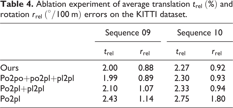
In this section, to verify the effectiveness of the proposed multiple weighted geometric loss, the network is retrained by combining different loss functions and subsequently tested on the same test sequence. The results are shown in Table 4. The results of combining multiple weighted geometric loss functions are better than those of any single method.

Table 4.

Ablation experiment of average translation $t_{rel} (%)$ and rotation $r_{rel} (° / 100 m)$ errors on the KITTI dataset.

	Sequence 09		Sequence 10
	$t_{rel}$	$r_{rel}$	$t_{rel}$	$r_{rel}$
Ours	2.00	0.88	2.27	0.92
Po2po+po2pl+pl2pl	1.99	0.89	2.30	0.93
Po2pl+pl2pl	2.10	1.07	2.33	0.94
Po2pl	2.43	1.14	2.75	1.80

Runtime

In the robot pose estimation process, the real-time performance of the algorithm is an important indicator. Commonly used LiDARs, such as the Velodyne HDL-64 LiDAR used in the KITTI and Apollo-SouthBay datasets, are set to 10 Hz, which means that one frame of scan data is output every 0.1 s. Therefore, real-time performance in this case means that the processing time of each data point is less than 0.1 s. Tested on a desktop computer equipped with Intel Xeon(R) CPU E5-2603V2 and NVIDIA GTX1080Ti GPU, the average data processing time per frame is 24 ms on CPU, and the inference time is 27 ms on GPU. The total pose estimation time of adjacent frames is 51 ms, which is less than 0.1 s and thus satisfies the real-time requirements of the algorithm.

Conclusions

This article presents an end-to-end self-supervised LiDAR odometry network for estimating the 6-DOF poses of a robot that does not require any data with pose labels to complete the training of the network. Geometric loss is used to learn domain-specific features during network training. The proposed method was validated on a public benchmark dataset and compared with other learning-based methods, and the method in this article showed excellent performance. The analysis shows that the learning-based method can overcome some of the shortcomings of the model-based method, but the accuracy cannot surpass that of the traditional LiDAR odometry method, and further research is required. In future work, we plan to add a long short-term memory model to the network to use time information and merge it with IMU data to build a multimodal end-to-end odometry framework.

Footnotes

Declaration of conflicting interests

The author(s) declared no potential conflicts of interest with respect to the research, authorship, and/or publication of this article.

Funding

The author(s) disclosed receipt of the following financial support for the research, authorship, and/or publication of this article: This work was supported by The National Natural Science Foundation of China (Grant No. 61803227, 61973184, 61773242), National Key Research and Development Plan of China (2020AAA0108903), Independent Innovation Foundation of Shandong University (Grant No. 2018ZQXM005), Young Scholars Program of Shandong University, Weihai (Grant No. 20820211010).

ORCID iD

Xu Fu

References

Yin

Wang

, et al. CoBigICP: robust and precise point set registration using correntropy metrics and bidirectional correspondence. In: 2020 IEEE/RSJ international conference on intelligent robots and systems (IROS), Las Vegas, NV, USA, 25–29 October 2020, pp. 4692–4699. IEEE.

Guo

Liu

, et al. 3D object recognition from cluttered and occluded scenes with a compact local feature. Mach. Vision Appl. 2019; 30(4): 763–783.

Bian

Wang

. Unsupervised scale-consistent depth and ego-motion learning from monocular video. In: 2019 neural information processing systems (NIPS), Vancouver, Canada, 08–14 December 2019, pp. 35–45. NIPS.

Guan

Cao

Chen

, et al. A real-time semantic visual SLAM approach with points and objects. Int J Adv Robot Syst 2020; 17(1): 1738062819.

Wang

Cao

, et al. Self-supervised deep visual odometry with online adaptation. In: 2020 proceedings of the IEEE/CVF conference on computer vision and pattern recognition (CVPR), Seattle, WA, USA, 13–19 June 2020, pp. 6339–6348. IEEE.

Zhai

, et al. JD-SLAM: Joint camera pose estimation and moving object segmentation for simultaneous localization and mapping in dynamic scenes. Int J Adv Robot Syst 2021; 18(1): 1739151823.

Chen

Wang

, et al. Lo-net: deep real-time LiDAR odometry. In: 2019 proceedings of the IEEE/CVF conference on computer vision and pattern recognition (CVPR), Long Beach, CA, USA, 15–20 June 2019, pp. 8473–8482. IEEE.

Wang

, et al. Self-supervised visual-LiDAR odometry with flip consistency. In: 2021 IEEE winter conference on applications of computer vision (WACV), Waikoloa, HI, USA, 3–8 January 2021, pp. 3844–3852. IEEE.

Zhang

Singh

. Low-drift and real-time LiDAR odometry and mapping. Auton Robot. 2017; 41(2): 401–416.

10.

Shan

Englot

. Lego-loam: lightweight and ground-optimized LiDAR odometry and mapping on variable terrain. In: 2018 IEEE/RSJ international conference on intelligent robots and systems (IROS), Madrid, ESP, 1–5 October 2018, pp. 4758–4765. IEEE.

11.

Wang

Xie

Intensity-SLAM: intensity assisted localization and mapping for large scale environment. IEEE Robot Autom Lett 2021; 6(2): 1715–1721.

12.

Yokozuka

Koide

Oishi

, et al. LiTAMIN: LiDAR-based tracking and MappINg by stabilized ICP for geometry approximation with normal distributions. In: 2020 IEEE/RSJ International Conference on Intelligent Robots and Systems (IROS), Las Vegas, NV, USA, 25–29 October 2020, pp. 5143–5150. IEEE.

13.

Jiao

Zhu

, et al. Robust odometry and mapping for multi-LiDAR systems with online extrinsic calibration. IEEE Trans Robot 2021: 1–10.

14.

Behley

Stachniss

. Efficient surfel-based SLAM using 3D laser range data in urban environments. In: Robotics: Science and Systems (RSS), Pittsburgh, PA, USA, 26-30 June 2018, IEEE.

15.

Wang

, et al. SLAM integrated mobile mapping system in complex urban environments. ISPRS J Photogramm 2020; 166: 316–332.

16.

Zheng

Zhu

. Efficient LiDAR odometry for autonomous driving. IEEE Robot Autom Lett 2021; 6(4): 8458–8465.

17.

Jiang

Chen

Guo

, et al. Novel indoor positioning algorithm based on LiDAR/inertial measurement unit integrated system. Int J Adv Robot Syst 2021; 18(2): 1739157299.

18.

Demim

Nemra

Louadj

. Robust SVSF-SLAM for unmanned vehicle in unknown environment. IFAC-PapersOnLine 2016; 49(21): 386–394.

19.

Mosbah

Demim

Mansoul

, et al. Simultaneous localization and mapping navigation of unmanned ground vehicle based on second-order smooth variable structure filter with improved technique to combat fading for advanced wireless communications. Proc Inst Mech Eng Part I-J Syst Control 2021; 235(7): 1258–1271.

20.

Fischer

Simon

Olsner

, et al. Stickypillars: robust and efficient feature matching on point clouds using graph neural networks. In: 2021 proceedings of the IEEE/CVF Conference on computer vision and pattern recognition (CVPR), Nashville, TN, USA, 20–25 June 2021, pp. 313–323. IEEE.

21.

Chen

Nardari

Lee

, et al. Sloam: semantic LiDAR odometry and mapping for forest inventory. IEEE Robot Autom Lett 2020; 5(2): 612–619.

22.

Yue

Zhao

, et al. Collaborative semantic understanding and mapping framework for autonomous systems. IEEE/ASME Trans Mecha 2020; 26(2): 978–989.

23.

, et al. LiDAR odometry and mapping based on semantic information for outdoor environment. Remote Sens-Basel 2021; 13(15): 2864.

24.

Wang

. DMLO: deep matching LiDAR odometry. In: 2020 IEEE/RSJ international conference on intelligent robots and systems (IROS), Las Vegas, NV, USA, 25–29 October 2020, pp. 6010–6017. IEEE.

25.

Chen

Milioto

Palazzolo

, et al. Suma++: efficient LiDAR-based semantic slam. In: 2019 IEEE/RSJ international conference on intelligent robots and systems (IROS), Macau, CHN, 3–8 November 2019, pp. 4530–4537. IEEE.

26.

Wang

Saputra

MRU

Zhao

, et al. Deeppco: end-to-end point cloud odometry through deep parallel neural network. In: 2019 IEEE/RSJ international conference on intelligent robots and systems (IROS), Macau, CHN, 3–8 November 2019, pp. 3248–3254. IEEE.

27.

Cho

Kim

. Unsupervised geometry-aware deep LiDAR odometry. In: 2020 IEEE international conference on robotics and automation (ICRA), Paris, France, 31 May–31 August 2020, pp. 2145–2152. IEEE.

28.

Nubert

Khattak

Hutter

. Self-supervised learning of LiDAR odometry for robotic applications. In: 2021 IEEE international conference on robotics and automation (ICRA), Xi’an, China, 30 May–5 June 2021, pp. 9601–9607. IEEE.

29.

Chen

Läbe

Milioto

, et al. OverlapNet: a Siamese network for computing LiDAR scan similarity with applications to loop closing and localization. Auton Robot 2021: 1–21.

Self-supervised learning of LiDAR odometry based on spherical projection

Abstract

Keywords

Introduction

Related work

Proposed approach

Problem statement

Input projection

Normal calculation

Network architecture

Loss function

Experimental results

Implementation details

Benchmark dataset

Experimental results

Evaluation on the KITTI dataset

Evaluation on the Apollo-SouthBay dataset

Evaluation on a real-world SLAM task

Ablation study

Runtime

Conclusions

Footnotes

Declaration of conflicting interests

Funding

ORCID iD

References