Sage Journals: Discover world-class research

Abstract

A cartridge 2D EHSV based on torque motor is proposed in this paper, which is keeping the advantages of conventional 2D valve, such as compact structure, high power-to-weight ratio, and excellent dynamic characteristics. In order to explore its dynamic characteristics, the design concept and operating principle of the cartridge 2D EHSV valve is presented first. Then the mathematical model of cartridge 2D EHSV valve is derived, especially the rotational viscous damping coefficient which is studied in detail. The simulation results of the open(closed)-loop model show that the support pressure plays an insignificant role in the dynamic characteristics of 2D EHSV, only the phase bandwidth of the closed-loop model increases. And the rise time of the open-loop model is about 10 ms, and the frequency bandwidth is about 40 Hz, while the rise time is about 4 ms and the frequency bandwidth is about 100 Hz of the closed-loop model. Furthermore, as verified by experimental results, the rising time of the step response is about 7 ms and the bandwidth is approximately 38 Hz under the open-loop control, while that is 6 ms and 117 Hz for 25% input signal under the close-loop control. Finally, the difference between the experiment and the simulation is discussed. It is concluded that the cartridge 2D EHSV has excellent dynamic characteristics.

Keywords

Cartridge valve 2D servo valve torque motor dynamic characteristics experimental research

Introduction

Electro-hydraulic servo valve (EHSV) is the core component of electro-hydraulic servo system.^1,2

It is a connection between electrical and hydraulic power, which plays an important role in the control accuracy and performance of the whole system.^3,4 The two most widely used servo valves are nozzle-flapper EHSV and jet pipe EHSV.^5,6 A mount of structural innovations and theoretical studies have been conducted on the two EHSV.

For reducing the influence of cavitation in the nozzle-flapper pilot stage on the stability and reliability of the valve, Aung and Li⁷ presented a simple and effective flapper shape, while Yang et al.⁸ proposed diamond nozzles to replace the traditional circular nozzles. Somashekhar et al.⁹ developed the mathematical model of a jet pipe EHSV with a built-in mechanical feedback, and simulated the steady state of it by using the finite element method. In order to explore conditions for high reliability, Wang and Yin¹⁰ proposed a dynamic model to describe the performance indicators of the jet pipe EHSV under random vibration environment.

The experimental results of EHSV is the only index to measure its merits. In order to test the dynamic characteristics of the servo valve accurately, Bensong and Keli¹¹ proposed a new test method, and the results show that the test system works well and the experimental data is reliable and effective. Yin et al.¹² established a mathematical model of jet pipe EHSV considering the eddy current effect, and obtained the influence of main parameters on the dynamic characteristics, and the model was verified its correctness through experiment. For exploring the mechanisms of action of several structure parameters on dynamic characteristics of jet deflector EHSV, Wang et al.¹³ presented a complete model and verified it by experiment. By combining the mathematical modeling and parameter identification, Shen and Cui¹⁴ derived a simulation model of EHSV. In order to improve the measurement accuracy of the dynamic characteristics of EHSV, Quan et al.¹⁵ proposed a novel calculation and a test rig, and the experiment results show that the measurement accuracy is about ±4%.

The theory of 2D pressure control valve and flow control valve were presented by Ruan at first,^16,17 which utilized both rotation and axial movement of a single spool. The rotation as the pilot stage, uses a spiral groove in the sleeve combined with high and low pressure holes on the spool land to control the pressure in the spool chamber, while the axial movement of the spool as the power stage is actuated by hydrostatic forces. The spool and sleeve which convert the rotation to the axial movement are called screw servo mechanism. On the basis of the theory, the theoretical and structural feasibility of 2D EHSV is studied. Zuo et al. proposed the 2D pressure EHSV,¹⁸ and explored its performance through experiments. The results show that the 2D pressure EHSV has good static and dynamic characteristics. Yi et al.¹⁹ presented and tested a 2D digital EHSV, which is composed of 2D EHSV and an embedded controller, the results show that the bandwidth of 2D digital servo valve is about 100 Hz.

The power-to-weight ratio (PWR) is one of the most critical indicators for EHSV, which as a fluid transmission component. On the basis of new design method, structure innovation and the utilize of new materials, the PWR of electric motor which as electrical transmission components has been greatly improved. In order to increased PWR of piezoelectric energy harvesters, Chandrasekharan and Thompson²⁰ proposed a honeycomb structures instead of the solid continuous substrate of conventional bimorph of the same material. Tounsi²¹ presented a motor-converter systemic design methodology improving its PWR, and validated by the finite elements and experimental methods. In contrast, the heavy sleeve of conventional EHSV is one of the essential factors limiting its PWR.

The cartridge design of valves is an important way to improve the PWR. It retains the original excellent performance, while discarding the heavy sleeve of conventional EHSV, which greatly reduces the weight of the valve. Compared with conventional valves, cartridge valves have many features, such as low-cost, leak-free, and large-flow capacity, which make them widely used in industrial and mobile machinery.²² However, the pilot stage and power stage of conventional EHSV are placed parallelly because of its structure limitation, so that the cartridge design of conventional EHSV only involves the power stage, resulting in the improvement of PWR being limited. On the contrary, the pilot stage and power stage of 2D EHSV are integrated on the same spool, so that it will achieve a more comprehensive cartridge design. In summary, it is necessary to design the cartridge valve, and the 2D EHSV has more advantages than conventional EHSV in terms of cartridge design.

In this paper, a cartridge-type 2D EHSV is presented, which installs the torque motor coaxially with the 2D spool and uses it as an electro-mechanical converter. Through structure introduction, mathematical modeling, simulation analysis, and experimental research, the characteristics of the cartridge 2D EHSV are explored. The results show that cartridge 2D EHSV has the advantages of simple structure, light weight, and good dynamic characteristics.

Structure and operating principle of cartridge 2D EHSV

Schematic structure

The structure and operating principle of cartridge 2D EHSV is shown in Figure 1. The overall size of the 2D EHSV is about 32 mm × 32 mm × 95 mm, which is smaller than the conventional 2D EHSV under the same design parameters. It mainly consists of torque motor and 2D valve. Torque motor consists of permanent magnets, iron block, armature, excitation coils, and hall sensor. The iron block and armature are made of high permeability material to reduce the loss of magnetic energy. The permanent magnets are distributed on both sides of the torque motor. The armature is surrounded by the excitation coils. For improving the control precision of the 2D EHSV, hall sensor is installed to feedback the displacement of the 2D spool in real time for realize the closed-loop control of the whole system. The 2D valve mainly includes the 2D spool and sleeve, wherein the 2D spool is coaxial connected with the armature. There are four ports produced by the cooperation of sleeve and the shoulder of the 2D spool, where P is the high-pressure port, A and B are the working ports, and T is the low-pressure port. There are high and low pressure groove on the 2D spool, where the low-pressure groove is connected directly with port T, while the high-pressure groove is connected with port P through the high-pressure hole and the internal flow channel of the 2D spool. The right end of the 2D spool and sleeve forms the sensitive chamber, while the left end forms the high-pressure chamber. It’s similar with the high-pressure groove that the high-pressure chamber is also connected with port P. The overlap area produced by the inclined groove which is on the sleeve, and high and low pressure groove on the 2D spool decides flow and pressure of the sensitive chamber.

Figure 1.

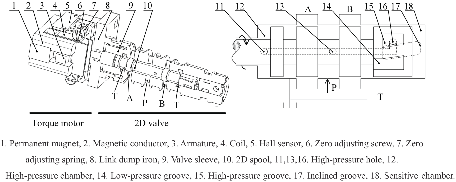
Schematic structure and operating principle of cartridge 2D EHSV.

Operating principle

As shown in Figure 1, high and low pressure groove are located on both sides of the inclined groove and form two parallelogram overlapping openings, which are connected in series to form a resistance bridge. The input pressure is the supply pressure, which is piloted to high-pressure groove and high-pressure chamber. The output pressure of the resistance bridge is fed to sensitive chamber. Under static conditions, there’s no output torque and the 2D spool has no rotation because of the symmetrical structure of torque motor when the excitation coil is not excited, the high-pressure groove has the same overlapping area with respect to the inclined groove as does the low-pressure groove; the resistance bridge gives an output pressure, which is half of that of port P, ported to the sensitive chamber. The area of the high-pressure chamber is designed to be half of that of the sensitive chamber. The 2D spool is in hydrostatic balance under these conditions.

When the coil is excited, the combined effect of the magnetic field generated by the permanent magnet and what generated by the excited coil will produce an output torque and drive the 2D spool to rotate, which changes the two parallelogram overlapping openings differentially, the pressure of the sensitive chamber shifts from its steady state, resulting in an imbalance in the hydrostatic force acting across the spool. This differential force causes the 2D spool to move axially. Movement of the 2D spool is such that the overlapping area between the high and low pressure groove and the inclined groove return to the symmetrical, as a result, a force balance is reestablished across the 2D spool.

For example, when the torque motor produces a clockwise output torque (The direction is shown in the Figure 1) the 2D spool rotates clockwise, the overlapping area between high-pressure groove and inclined groove increases, so that the pressure of sensitive chamber increases, the differential force causes the 2D spool moves axially to the left. When the 2D spool moves axially to the left, the port A connects with port P and port B connects with port T, the overlapping area between high-pressure groove and inclined groove grows smaller, while the overlapping area between low-pressure groove and inclined groove grows larger, the pressure of sensitive chamber decreases. When the pressure in the sensitive chamber goes down to be equal to half of that in the high-pressure chamber, the 2D spool reaches equilibrium position and stops moving, and the opening of ports is no longer changed. On the contrary, When the torque motor produces counterclockwise output torque, the 2D spool will produce a axial movement to the right until a new equilibrium is reached.

Mathematical model of cartridge 2D EHSV

There are two kinds of motion in the operation of the 2D EHSV, which are rotation and axial movement, so that the mathematical modeling will be carried out for these two kinds of motion respectively.

Mathematical model of rotation

The output torque of torque motor causes the rotation of 2D spool-armature assembly, so the output torque will be analyzed.

Linearity is one of the main criteria of torque motor. The torque equation of torque motor is:²³

T_{d} = K_{t} i + K_{m} θ

(1)

K_{t} = \frac{a M_{p} μ_{0} A_{g}}{g^{2}} N_{c}

(2)

K_{m} = \frac{a^{2} M_{p}^{2} μ_{0} A_{g}}{g^{3}}

(3)

where T_d is output torque of torque motor, K_t is torque constant of the torque motor, i is the current of coil, K_m is magnetic spring constant of torque motor, θ is rotary angle of armature, a is the rotational radius of the armature, M_p is magnetic potential generated by permanent magnets, µ₀ is the permeability of air, Ag is effective area of magnetic conductor at the air gap, g is the initial length of air gap, N_c is the number of coil turns.

The expressions of K_t and K_m have been derived in detail in reference 18, which will not be repeated in this paper.

The kinetic equation of torque motor arises by applying Newton’s second law to the torques on 2D spool-armature assembly is:

T_{d} = J_{a} \frac{d^{2} θ}{d t^{2}} + B_{a} \frac{d θ}{dt} + K_{a} θ + T_{L}

(4)

where J_a is inertia moment of 2D spool-armature assembly, B_a is the total rotational viscous damping coefficient, including two parts, which will be discussed in detail in the next section, K_a is mechanical torsion spring constant of 2D spool-armature assembly, T_L is load torque on 2D spool-armature assembly.

The block diagram of rotation can be obtained from equations (1) and (4):

According to Figure 2, the mathematical model of rotation can be derived as equation (5).

θ (s) = \frac{\frac{K_{t}}{K_{a} - K_{m}} i (s) - \frac{1}{K_{a} - K_{m}} T_{L}}{\frac{s^{2}}{ω_{m}^{2}} + \frac{2 ξ_{m}}{ω_{m}} s + 1}

(5)

ω_{m} = \sqrt{\frac{K_{a} - K_{m}}{J_{a}}}

(6)

ξ_{m} = \frac{B_{a}}{2 \sqrt{J_{a} (K_{a} - K_{m})}}

(7)

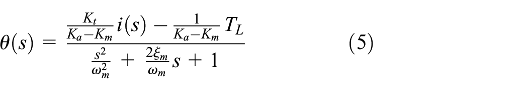
where ω_m is the natural frequency of torque motor, ξ_m is the damping coefficient of torque motor.

Figure 2.

Block diagram of rotation.

Analysis of total rotational viscous damping coefficient

There are two parts from the rotational viscous damping coefficient: the frictional viscous damping coefficient B_a₁ caused by the rotary shear flow between 2D spool and sleeve, and the rotational viscous damping coefficient B_a₂ caused by the transient hydraulic torque, which is caused by the rotation of the 2D spool pilot stage. The total rotational viscous damping coefficient is the sum of them.

Analysis of the frictional viscous damping coefficient

Figure 3 shows the schematic diagram of rotational shear flow between the 2D spool and valve sleeve. As the 2D spool rotates relative to the valve sleeve, the oil performs a rotating shear flow in the gap. It can be regarded as parallel flow because of the gap height is far less than the 2D spool radius.

Figure 3.

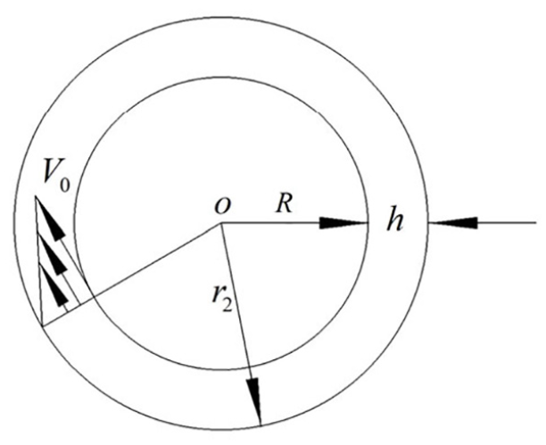
Schematic diagram of rotational shear flow.

The friction is evenly distributed along the gap height

τ = \frac{μ V_{0}}{h}

(8)

The frictional moment is

M = μ \frac{π L}{h} \frac{d^{3}}{4} \frac{d θ}{dt}

(9)

So the frictional viscous damping coefficient is

B_{a 1} = μ \frac{π L}{h} \frac{d^{3}}{4}

(10)

where µ is the dynamic viscous of the oil, d is the diameter of the 2D spool, h is the gap height, L is the contact length of rotary shear flow between the 2D spool and valve sleeve.

Analysis of the rotational viscous damping coefficient

During the rotation of 2D spool-armature assembly, the change of the overlap area between the high (low)-pressure groove and the inclined groove changes the flow between them, and the oil velocity in the high (low)-pressure groove will be changed, and there will generate a transient hydraulic torque on the 2D spool.

According to the design requirements, the unilateral maximum rotation angle of the 2D spool is 1° (Rotate clockwise as the positive direction). The special operating principle of the cartridge 2D EHSV determines that the transient hydraulic force needs to be analyzed separately.

The transient hydraulic torque between the high-pressure groove and the inclined groove is considered first. Figure 4 shows that the transient hydraulic torque between the high-pressure groove and the inclined groove.

Figure 4.

Transient hydraulic torque between the high-pressure groove and the inclined groove: (a) from 0° to 1° and (b) from 1° to 0°.

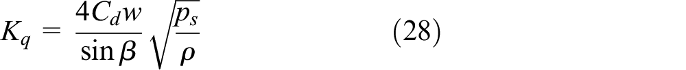
According to the working principle of cartridge 2D EHSV, the flow flux from the high-pressure groove to the inclined groove is

Q_{1} = C_{d} A_{1} \sqrt{\frac{2}{ρ} (p_{s} - p_{c})}

(11)

where C_d is flow coefficient, $A_{1}$ is the overlap area between high-pressure groove and inclined groove, ρ is density of hydraulic oil, p_s is pressure of system, p_c is pressure of sensitive chamber.

The overlapping area between high-pressure groove and inclined groove can be derived as equation (12).

A_{1} = - 2 R θ w + \frac{2 w h_{0}}{\sin β}

(12)

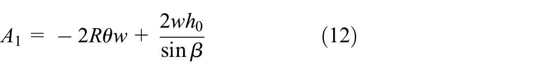
where R is radius of the 2D spool, w is width of the high-pressure groove, θ is the rotation angle of the 2D spool, h₀ is the initial overlap height between the high-pressure groove and inclined groove, β is the angle of inclined groove.

Based on the concept of the transient hydraulic force, we have

F_{t 1} = ρ L_{1} \frac{d (Q_{1})}{dt}

(13)

where L₁ is the damping length between the high-pressure groove and the inclined groove.

From equations (11) to (13), the transient hydraulic torque can be described as equation (14).

T_{t 1} = F_{t 1} \cdot R = C_{d} L_{1} WR \sqrt{2 ρ (p_{s} - p_{c})} \frac{d θ}{dt}

(14)

where W is the area gradient of the overlap area between the high-pressure groove and the inclined groove.

The damping length in Figure 4(a) and (b) is equal in magnitude and opposite in direction, while it is positive in Figure 4(a), which means that the rotational viscous damping coefficient is positive in Figure 4(a).

So the rotational viscous damping coefficient is

B_{a 2} = {\begin{matrix} C_{d} L_{1} WR \sqrt{2 ρ (p_{s} - p_{c})} & 0 ° \to 1 ° \\ - C_{d} L_{1} WR \sqrt{2 ρ (p_{s} - p_{c})} & 1 ° \to 0 ° \end{matrix}

(15)

Figure 5 shows that the transient hydraulic torque between the low-pressure groove and the inclined groove.

Figure 5.

Transient hydraulic torque between the inclined groove and the low-pressure groove: (a) from 0° to −1° and (b) from −1° to 0°.

Similarly, the flow flux from the inclined groove to the high-pressure groove is

Q_{2} = C_{d} A_{2} \sqrt{\frac{2}{ρ} p_{c}}

(16)

where A₂ is the overlap area between the low-pressure groove and the inclined groove.

The overlapping area between low-pressure groove and inclined groove can be derived as equation (17).

A_{2} = 2 R θ w + \frac{2 w h_{0}}{\sin β}

(17)

The transient hydraulic torque between the inclined groove and the low-pressure groove can be deduced as equation (18).

T_{t 2} = F_{t 2} \cdot R = C_{d} L_{2} WR \sqrt{2 ρ p_{c}} \frac{d θ}{dt}

(18)

where L₂ is the damping length between the high-pressure groove and the inclined groove.

Similar to Figure 4, the damping length in Figure 5(a) and (b) is also of equal magnitude and opposite direction, while it is positive in Figure 5(b).

So we have

B_{a 2} = {\begin{matrix} - C_{d} L_{2} WR \sqrt{2 ρ p_{c}} & 0 ° \to - 1 ° \\ C_{d} L_{2} WR \sqrt{2 ρ p_{c}} & - 1 ° \to 0 ° \end{matrix}

(19)

Combined with equations (10), (15), and (19), the total rotational viscous damping coefficient is

B_{a} = μ \frac{π L}{h} \frac{d^{3}}{4} + {\begin{matrix} C_{d} L_{1} WR \sqrt{2 ρ (p_{s} - p_{c})} & 0 ° \to 1 ° \\ - C_{d} L_{1} WR \sqrt{2 ρ (p_{s} - p_{c})} & 1 ° \to 0 ° \\ - C_{d} L_{2} WR \sqrt{2 ρ p_{c}} & 0 ° \to - 1 ° \\ C_{d} L_{2} WR \sqrt{2 ρ p_{c}} & - 1 ° \to 0 ° \end{matrix}

(20)

Mathematical model of axial movement

The axial movement of 2D spool-armature assembly is caused by the hydraulic force which is generated by pressure changes in the sensitive chamber of the 2D spool.

Based on the flow continuity principle, the flow equation of sensitive chamber is

Q_{1} - Q_{2} = A_{s} \frac{d x_{v}}{dt} + \frac{V_{c}}{β_{e}} \frac{d p_{c}}{dt}

(21)

where A_s is working area of sensitive chamber, xv is axial displacement of the 2D spool, V_c is volume of sensitive chamber, β_e is bulk modulus of hydraulic oil.

The motion equation of 2D spool-armature assembly is

p_{c} A_{s} - p_{s} A_{L} = m \frac{d^{2} x_{v}}{d t^{2}} + B_{s} \frac{d x_{v}}{dt} + K_{s} x_{v} + F_{L}

(22)

where A_L is working area of high-pressure chamber, m is 2D spool-armature assembly mass, B_s is axial viscous damping coefficient, K_s is axial spring constant of 2D spool-armature assembly, F_L is load force on 2D spool-armature assembly.

The axial movement of 2D spool-armature assembly is caused by its rotation. The variation of overlap height between high-pressure groove and inclined groove (Δh) is

Δ h = R θ \sin β - x_{v} \cos β

(23)

From equations (21) to (23), the block diagram of the axial movement can be described as Figure 6.

Figure 6.

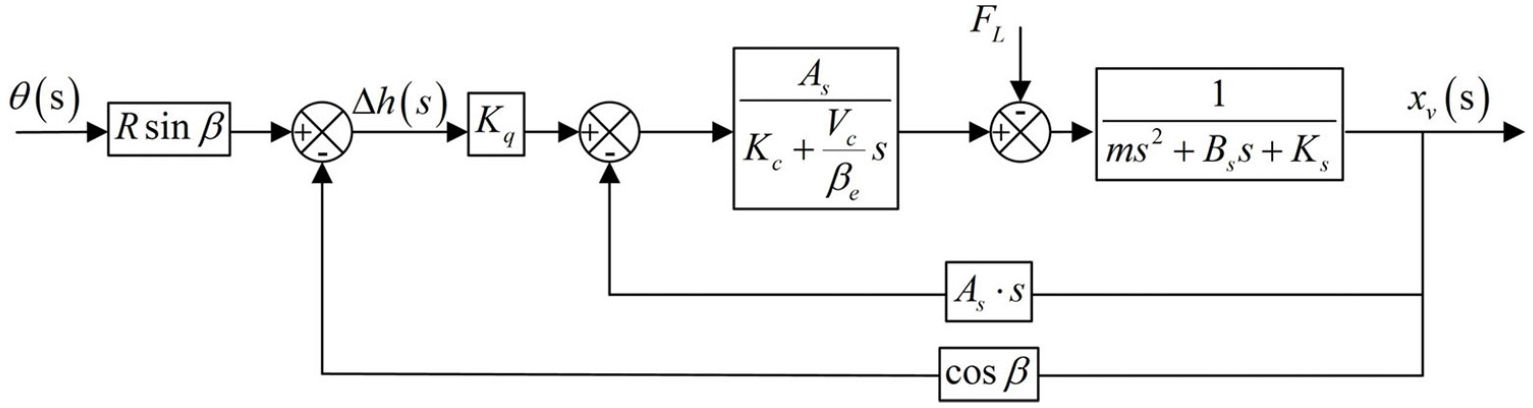
Block diagram of axial movement.

According to the actual parameters, we have

\frac{V_{c} K_{s}}{β_{e} A_{s}^{2}} + \frac{K_{c} B_{s}}{A_{s}^{2}} = 1, \frac{K_{c} K_{s}}{A_{s}^{2}} \approx 0

(24)

According to Figure 6 and equation (24), it can be obtained that the partial transfer function is

\frac{x_{v} (s)}{Δ h (s)} = \frac{K_{q} / A_{s}}{s (\frac{s^{2}}{ω_{h}^{2}} + \frac{2 ξ_{h} s}{ω_{h}} + 1)}

(25)

ω_{h} = \sqrt{\frac{β_{e} A_{s}^{2}}{m V_{c}}}

(26)

ξ_{h} = \frac{K_{c} \sqrt{\frac{β_{e} m}{V_{c}}}}{2 A_{s}} + \frac{B_{s} \sqrt{\frac{V_{c}}{β_{e} m}}}{2 A_{s}}

(27)

K_{q} = \frac{4 C_{d} w}{\sin β} \sqrt{\frac{p_{s}}{ρ}}

(28)

K_{c} = \frac{4 C_{d} h_{0} w}{\sin β \sqrt{ρ p_{s}}}

(29)

where K_q is the flow gain, K_c is the pressure-flow coefficient, ω_h is the hydraulic natural frequency, ξ_h is the hydraulic damping coefficient.

Since the bulk modulus of hydraulic oil has a large order of magnitude, the hydraulic natural frequency ω_h is far larger than the working bandwidth of the cartridge 2D EHSV, thus equation (25) can be simplified as equation (30)

\frac{x_{v} (s)}{Δ h (s)} = \frac{K_{q} / A_{s}}{s}

(30)

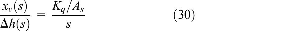
The closed-loop transfer function of the axial movement is

\frac{x_{v} (s)}{θ (s)} = \frac{R \cdot \tan β}{\frac{A_{s}}{K_{q} \cdot \cos β} s + 1}

(31)

Mathematical model of cartridge 2D EHSV

When the hall sensor has no displacement feedback, the cartridge 2D EHSV is under the open-loop control, and the open-loop block diagram of can be described as Figure 7 by combining equations (1) to (31).

Figure 7.

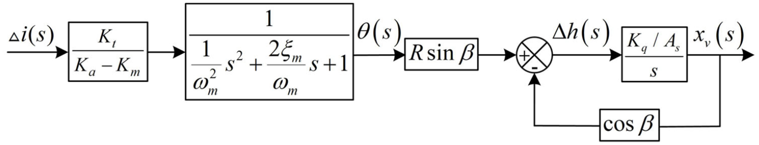
The open-loop block diagram of cartridge 2D EHSV.

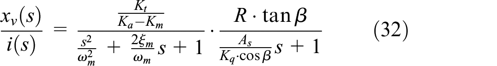
And the model without displacement feedback (named open-loop model) can be derived from Figure 7, as shown in equation (32).

\frac{x_{v} (s)}{i (s)} = \frac{\frac{K_{t}}{K_{a} - K_{m}}}{\frac{s^{2}}{ω_{m}^{2}} + \frac{2 ξ_{m}}{ω_{m}} s + 1} \cdot \frac{R \cdot \tan β}{\frac{A_{s}}{K_{q} \cdot \cos β} s + 1}

(32)

On the contrary, when there is displacement feedback from the hall sensor and the cartridge 2D EHSV is under the closed-loop control. The PID algorithm in the controller will reduce the error between the displacement of and the input signal. The expression of the PID algorithm is shown as equation (33)

P + I \frac{1}{s} + D \frac{N}{1 + N \frac{1}{s}}

(33)

where P is proportional coefficient, I is integral time constant, D is derivative coefficient, N is filter coefficient.

So the closed-loop block diagram can be obtained as shown in Figure 8.

Figure 8.

The closed-loop block diagram of cartridge 2D EHSV.

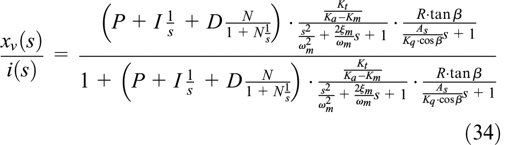
The model with displacement feedback (named closed-loop model) can be derived as equation (34).

\frac{x_{v} (s)}{i (s)} = \frac{(P + I \frac{1}{s} + D \frac{N}{1 + N \frac{1}{s}}) \cdot \frac{\frac{K_{t}}{K_{a} - K_{m}}}{\frac{s^{2}}{ω_{m}^{2}} + \frac{2 ξ_{m}}{ω_{m}} s + 1} \cdot \frac{R \cdot \tan β}{\frac{A_{s}}{K_{q} \cdot \cos β} s + 1}}{1 + (P + I \frac{1}{s} + D \frac{N}{1 + N \frac{1}{s}}) \cdot \frac{\frac{K_{t}}{K_{a} - K_{m}}}{\frac{s^{2}}{ω_{m}^{2}} + \frac{2 ξ_{m}}{ω_{m}} s + 1} \cdot \frac{R \cdot \tan β}{\frac{A_{s}}{K_{q} \cdot \cos β} s + 1}}

(34)

Simulation analysis

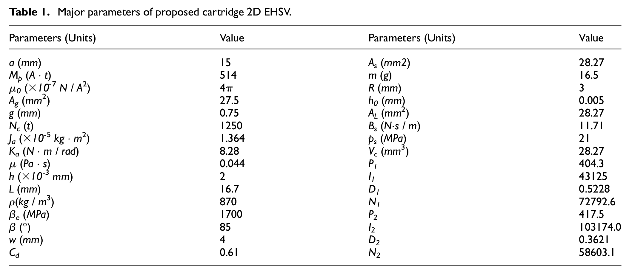
The mathematical model of the 2D EHSV under open (closed)-loop is validated through simulation, and the major parameters are listed in Table 1, where P₁–N₁ are parameters of the open-loop model, while P₂–N₂ are parameters of the closed-loop model.

Table 1.

Major parameters of proposed cartridge 2D EHSV.

Parameters (Units)	Value	Parameters (Units)	Value
a (mm)	15	A_s (mm2)	28.27
M_p (A · t)	514	m (g)	16.5
µ₀ (×10^-7N / A²)	4 \pi	R (mm)	3
A_g (mm²)	27.5	h₀ (mm)	0.005
g (mm)	0.75	A_L (mm²)	28.27
N_c (t)	1250	B_s (N·s / m)	11.71
J_a (×10^-5kg · m²)	1.364	p_s (MPa)	21
K_a (N · m / rad)	8.28	V_c (mm³)	28.27
µ (Pa · s)	0.044	P₁	404.3
h (×10^-3mm)	2	I₁	43125
L (mm)	16.7	D₁	0.5228
ρ(kg / m³)	870	N₁	72792.6
β_e (MPa)	1700	P₂	417.5
β (°)	85	I₂	103174.0
w (mm)	4	D₂	0.3621
C_d	0.61	N₂	58603.1

The comparison of step response of open-loop and closed loop model under different support pressure is shown in Figure 9. As shown in Figure 9, all of the curves are over-damped and with the change of support pressure, the rise time of 2D EHSV almost remains unchanged. The rise time of the open-loop model is about 10 ms, while that is about 4 ms of the closed-loop model.

Figure 9.

Comparison of step response curve between open-loop and closed-loop model: (a) under open-loop and (b) under closed-loop.

Figure 10(b) shows the frequency response curve that the amplitude bandwidth (−3 dB) is about 40 Hz and the phase bandwidth (−90°) is approximately 70 Hz under the closed-loop control, while the amplitude bandwidth (−3 dB) is about 120 Hz and the phase bandwidth is about 200 Hz under the open-loop control.

Figure 10.

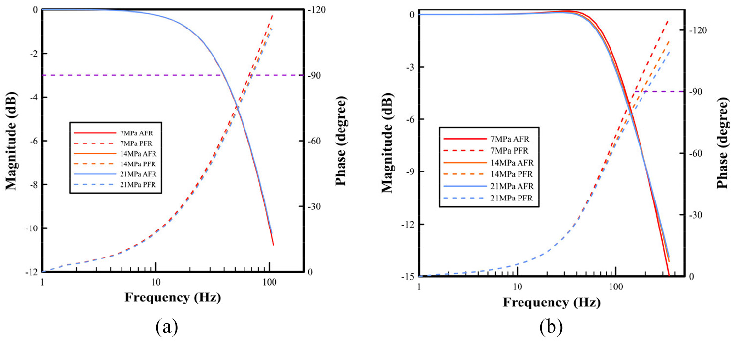
Comparison of frequency response curve between open-loop and closed-loop model: (a) under open-loop and (b) under closed-loop.

Figure 10 is the simulation results of frequency response of the two mathematical models. It is similarly with Figure 9, the changes of support pressure play an insignificant role in the frequency response of open-loop model in Figure 10(a), and the amplitude bandwidth (−3 dB) is about 40 Hz, the phase bandwidth (−90°) is approximately 70 Hz.

The frequency response of the closed-loop under different support pressure is shown in Figure 10(b). The amplitude bandwidth (−3 dB) is about 100 Hz while the phase bandwidth (−90°) is about 200 Hz when the support pressure is 21 MPa. It is different from open-loop model, when the support pressure increases, the phase bandwidth increases from 160 Hz to 200 Hz, while the amplitude bandwidth is nearly constant.

It can be seen from the simulation results that the closed-loop model of cartridge 2D EHSV has better dynamic characteristics.

Research prototype and experimental investigation

Development of research prototype

A research prototype is developed for experimental purpose in Figure 11(a). Figure 11(b) shows the test rig of cartridge 2D EHSV which includes pump, signal generator, oscilloscope, research prototype, controller, and pressure gauges. The pump provides a system pressure of 21 MPa for the research prototype, the pressure gauges are installed for monitoring the pressure of port A, B, P, and T. The controller is the connection between the Hall sensor and the research prototype and provides PID control. The signal generator is used to generate input signals of different waveforms, and the waveforms of the input signal and the 2D spool displacement will be displayed on the oscilloscope.

Figure 11.

Test rig of cartridge 2D EHSV: (a) the research prototype of cartridge 2D EHSV, (b) test rig overview for the measurement of dynamic characteristics, and (c) schematic diagram of test rig.

Experimental method

The dynamic characteristics of the research prototype, which includes the step response and the frequency response are tested under open-loop and closed-loop control on the test rig.

The method of the step response performance

The signal generator sends the input current signal in the form of square wave to the coil, and the research prototype would move correspondingly. There are two signal waves connected into the oscilloscope, include the output displacement signal which is monitored by the hall sensor, and the input signal. (The output flow signal is replaced by the displacement signal of the 2D spool, because of the linear relationship between the two signals.) And the step response curve could be drawn from the waveform data of the input signal and output signal obtained by the oscilloscope.

The method of the frequency response performance

There are a series of different frequency sinusoidal current signals generated by the signal generator, which makes the research prototype move correspondingly. The wave of input signal and output signal would be connected into the oscilloscope, and the data of the two signals is also recorded. And the amplitude of the output signal at 1 Hz which is regarded as reference, is calculated logarithmically with that of each tested frequency, so that the amplitude frequency curve could be plotted by the results of the logarithm calculation. The phase frequency curve is drawn by a series of lagging phase difference which is obtained by comparing the waveform of input and output signal at tested frequency.

Experimental investigation

The comparison of simulation and experimental results are presented in Figures 11 and 12.

Figure 12.

Comparison between experimental results and simulation (open-loop): (a) step response curve and (b) frequency response curve.

Figure 12 shows the comparison between experimental and simulation results under the open-loop control. Figure 12(a) shows that the rising time of experimental curve is about 7 ms. There’s no overshoot but some oscillations in the experimental curve. It might be caused by the effect of the rotational angular of 2D spool on the measurement of Hall sensor. Figure 12(b) shows the frequency response characteristics that the amplitude bandwidth of the cartridge 2D EHSV is about 38 Hz (−3 dB) and the phase bandwidth is approximately 70 Hz (−90°) in the experimental curve.

Figure 13 shows the comparison between experimental results and simulation under the closed-loop control. Figure 13(a) shows that the rising time of experimental curve is about 6 ms, while which is about 4 ms of simulation curve. Similar with the open-loop case, there are also oscillations in the experimental results under the closed-loop control, which is caused by the PID regulating effect. Figure 13(b) shows the frequency response characteristics that the amplitude bandwidth of the cartridge 2D EHSV is about 117 Hz (−3 dB) and the phase bandwidth is approximately 180 Hz (−90°) in the experimental curve. There are some deviations between the experimental curve and simulation curve in the low frequency part of the phase-frequency characteristic curve, which may be caused by ignoring the effect of magnetic flux leakage when deriving the mathematical model.

Figure 13.

Comparison between experiment results and simulation (closed-loop): (a) step response curve and (b) frequency response curve.

Experiment results

According to the experiment results, when the support pressure is 21 MPa and under 25% input signal, the closed-loop dynamic characteristics of 2D EHSV and those of “MOOG D662-P” are shown in Table 1. It can be seen that the dynamic characteristics of the two EHSVs are similarly, and the 2D EHSV has slight advantages in some parameters, see Table 2.

Table 2.

The dynamic characteristics of two EHSV.

	2D EHSV	MOOG D662-P
Step response	6 ms	9 ms
Magnitude bandwidth	117	100 Hz
Phase bandwidth	180 Hz	100 Hz

Conclusions

A new cartridge 2D EHSV which uses torque motor as electro-mechanical converter is proposed in this paper to achieve the cartridge design and reduce the overall size, while maintaining the excellent of the 2D EHSV. The major work of this paper includes:

The mathematical models with and without displacement feedback of the cartridge 2D EHSV, which named closed-loop and open-loop model are formulated by considering its operating principle. The rotational viscous damping coefficient is studied analytically, which is different from the conventional method of parameter identification. The simulation results show that the closed-loop model has better dynamic characteristics than the open-loop model, and the support pressure has little effect on dynamic characteristics of 2D EHSV.

A research prototype has been developed for verification of the correctness of simulation results, and a test rig for experimental purpose has been developed. In the step response experiment, the rising time is about 7 ms under the open-loop control, while it is about 6 ms under the closed-loop control. Experimental and simulation results are consistent, but there are some oscillations in both experimental curves, the oscillations in the open loop curve may be caused by the position feedback of the 2D spool or the damping coefficient of the axial movement is too small, while that in the closed loop curve may be caused by the position feedback and the PID adjustment.

In the frequency characteristic experiment, the amplitude bandwidth is about 38 Hz and the phase bandwidth is about 70 Hz when there’s no displacement feedback, while when there is displacement feedback, the amplitude bandwidth is about 117 Hz and the phase bandwidth is approximately 180 Hz. There are some deviations between experimental and simulation curve in low frequency part of the phase-frequency response curve under the closed-loop control, which may be caused by ignoring the effect of magnetic flux leakage. In order to verify these conjectures, there will be more investigation of the cartridge 2D EHSV.

The experimental results verify the correctness of the simulation, and show that the dynamic characteristics of cartridge 2D EHSV is not weaker than “MOOG D662-P.”

Footnotes

Handling Editor: James Baldwin

Declaration of conflicting interests

The author(s) declared no potential conflicts of interest with respect to the research, authorship, and/or publication of this article.

Funding

The author(s) received no financial support for the research, authorship, and/or publication of this article.

ORCID iD

Fei-Xia Zheng

References

Zhang

Yan

Duan

, et al. High torque density torque motor with hybrid magnetization pole arrays for jet pipe servo valve. IEEE Trans Ind Electron 2019; 67: 2133–2142.

Xiaofeng

Xianglin

Longjun

, et al. Optimization and simulation on a cartridge valve with silencing grooves. J Vib Control 2014; 20: 2083–2089.

Chu

Yuan

Chen

. Research on dynamic reliability of a jet pipe servo valve based on generalized stochastic Petri nets. Int J Aerosp Eng 2015; 2015: 171642.

Yan

Zhang

, et al. Numerical simulation and experimental research of the flow force and forced vibration in the nozzle-flapper valve. Mech Syst Signal Process 2018; 99: 550–566.

Somashekhar

Singaperumal

Kumar

. Modelling the steady-state analysis of a jet pipe electrohydraulic servo valve. Proc Inst Mech Eng Part I-J Syst Control Eng 2006; 220: 109–130.

Zhang

Aung

. Reduction of undesired lateral forces acting on the flapper of a flapper-nozzle pilot valve by using an innovative flapper shape. Energy Conv Manag 2015; 106: 835–848.

Aung

. A numerical study of cavitation phenomenon in a flapper-nozzle pilot stage of an electrohydraulic servo-valve with an innovative flapper shape. Energy Conv Manag 2014; 77: 31–39.

Yang

Wang

. Numerical simulations on flow characteristics of a nozzle-flapper servo valve with diamond nozzles. IEEE Access 2019; 7: 28001–28010.

Somashekhar

Singaperumal

Kumar

. Mathematical modelling and simulation of a jet pipe electrohydraulic flow control servo valve. Proc Inst Mech Eng Part I-J Syst Control Eng 2007; 221: 365–382.

10.

Wang

Yin

. Performance reliability of jet pipe servo valve under random vibration environment. Mechatronics 2019; 64: 13.

11.

Bensong

Keli

. Research on frequency response experiment of servo valve based on LabVIEW. IOP Conf Ser Earth Environ Sci 2019; 310: 032024.

12.

Yin

Guo

, et al. Modeling and frequency characteristics of jet-pipe servo valve considering eddy current effect. J Aerosp Power 2020; 35: 1777–1785.

13.

Wang

Zuo

Yan

, et al. Dynamic modeling and characteristics investigation of jet deflector servo valve. Acta Armamentarii 2018; 39: 598–607.

14.

Shen

Cui

. Simulation modeling of static and dynamic property of hydraulic proportional servo valve. Comput Simul 2015; 32: 236–240.

15.

Quan

Sheng

Chen

. Dynamic performance test of electro-hydraulic servo valve based on joint test and control. Trans Chinese Soc Agric Mach 2016; 47: 377–382.

16.

Ruan

Burton

Ukrainetz

, et al. Two-dimensional pressure control valve. Proc Inst Mech Eng Part C: J Mech Eng Sci 2001; 215: 1031–1038.

17.

Ruan

Burton

Ukrainetz

. An investigation into the characteristics of a two dimensional “2D” flow control valve. J Dyn Sys Meas Control 2002; 124: 214–220.

18.

Zuo

Liu

Zhang

, et al. Design and characteristics analysis of bourdon tube pressure feedback for 2D pressure servo valve. Comptes Rendus De l Academie Bulgare Des Sciences 2018; 71: 92–98.

19.

Ruan

. Frequency response of 2D digital servo valve. Mach Tool Hydraulics 2009; 11.

20.

Chandrasekharan

Thompson

. Increased power to weight ratio of piezoelectric energy harvesters through integration of cellular honeycomb structures. Smart Mater Struct 2016; 25: 17.

21.

Tounsi

. Systemic design and optimization improving performances of permanent magnet motors. Int J Electr Compon Energy Convers 2015; 1: 1–15.

22.

Kong

Wei

Yan

. Application of flow field decomposition and reconstruction in studying and modeling the characteristics of a cartridge valve. Eng Appl Comput Fluid Mech 2018; 12: 385–396.

23.

Merritt

. Hydraulic control systems. J Wiley, 1967.

Theoretical and experimental research on the cartridge two-dimensional (2D) electro-hydraulic servo valve

Abstract

Keywords

Introduction

Structure and operating principle of cartridge 2D EHSV

Schematic structure

Operating principle

Mathematical model of cartridge 2D EHSV

Mathematical model of rotation

Analysis of total rotational viscous damping coefficient

Analysis of the frictional viscous damping coefficient

Analysis of the rotational viscous damping coefficient

Mathematical model of axial movement

Mathematical model of cartridge 2D EHSV

Simulation analysis

Research prototype and experimental investigation

Development of research prototype

Experimental method

The method of the step response performance

The method of the frequency response performance

Experimental investigation

Experiment results

Conclusions

Footnotes

Declaration of conflicting interests

Funding

ORCID iD

References