
Abstract
The car-following model has always been a research hot spot in the field of traffic flow theory. Modeling the car-following behavior can quantify the longitudinal interaction between cars, thereby understanding the characteristics of traffic flow, and revealing the inherent mechanisms of traffic congestion and other traffic phenomena. In fact, there is an asymmetry problem in the driver’s acceleration and deceleration operation. The existing car-following model ignores the difference between the acceleration and deceleration of cars. To solve this problem, the cars driving on the road are compared to molecules with interactions. Based on the molecular interaction potential function and the wall potential function, we construct a molecular car-following model. We use NGSIM data set to calibrate the parameters of the model through the genetic algorithm. Finally, we analyze the evolution rule of the disturbance in the traffic flow in different states with the help of the time-space diagram, and compare the molecular model and the classical optimal velocity model. The results show that the molecular car-following model can better describe the car-following behavior from the micro level.
Introduction
Car-following behavior is a very important part of traffic safety, and the research on its model has been constantly improved and improved. The concept of car-following originated from the early 1950s and was proposed by Pipes. 1 From the micro level, car-following behavior describes the interaction between two adjacent workshops in a single lane car fleet with limited overtaking. For more than 60 years, scholars have carried out systematic research on car-following model. Scholars in various fields try to explain the observed micro phenomena from different perspectives.2,3 There are many kinds of car-following models. According to their starting point, they can be divided into two categories: data driven and theory driven.
Data driven model: this kind of model uses the method of intelligent calculation to build car-following model to fit a large number of high-precision data of car trajectory. This kind of model does not have very clear physical meaning, but in practical application, it can give some explanation and prediction for some complex traffic phenomena which cannot be simulated by theoretical driven models. 4 In 1986, Rumelhart put forward BP (Back Propagation) neural network, 5 which is a multi-tier FNN (Feed forward Neural Network). It uses the error back propagation algorithm to adjust the weight, and it is the most widely used neural network model at present. With the wide application of a neural network in the field of traffic simulation, Kehtarnavaz et al. 6 first applied the BP neural network model to the modeling of car-following behavior in 1998. The input of the model was the speed of follower and the distance between two cars, and the output was the relative speed of two cars, and its validity was verified. Jia et al. 7 also established a car-following model based on BP neural network, whose input is the speed of following car, the relative speed of two cars, the distance between two cars and the expected distance between cars, and the output is the acceleration of follower. However, in the process of training, BP neural network model cannot predict the extreme value (such as acceleration equal to zero) with small error. Moreover, because this kind of model is not introduced into the theory of car following, its simulation may even have errors.8,9 Subsequently, support vector regression(SVR) was used to study car-following behavior. SVR 10 is an algorithm in machine learning. It transforms the original problem into a convex quadratic programming problem, which can be solved by using the optimization theory to obtain the global optimal solution and the kernel function is introduced, and the input space is mapped to a feature space through a mapping function of nonlinear transformation, thus avoiding the “dimension disaster.” In 2010, Wei and Liu 11 first proposed a car-following model based on support vector regression. Its input was the speed of follower at the current time, the relative speed of two cars and the distance between two cars, and the output is the following car’s speed at the next time. The evaluation index shows that the model has a good simulation effect. After that, with the emergence of online traffic simulation technology, Wang and Chen 12 established a car-following model based on online support vector regression. Theoretically, the effect of using support vector regression to model car-following behavior is better, but the research based on this kind of model is still in its infancy, and there are few related achievements.
Theory driven model: it is a model based on the relevant theory of car-following behavior and the knowledge of dynamics. The physical meaning of this model is clear, and it has been applied in many traffic simulation software. In the development of theory driven models, the stimulus-response model is the most classical car-following model, and GM (General Motors) model 13 is the most important one. Since the late 1950s, many stimulus-response models have been built on the basis of the GM model. GM model assumes that the car does not overtake or change lanes when driving in the following direction. It is derived from driving dynamics theory, and its basic formula is as follows:
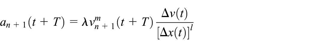
Where
However, it is easy to change with the change of traffic operation state, so it is not universal. For this reason, Newell 14 proposed a new car-following model in 1961, which adjusted the velocity to an optimal velocity depending on the headway, which also laid a foundation for the later optimal velocity (OV) model. As a widely used car-following model, the OV model can reasonably describe the instability of traffic flow and the evolution process of different congestion levels from a macro perspective, but the model is based on the expression of the acceleration of the car-following, and there are some shortcomings: in the simulation process, the velocity data of some cars will appear negative values, and there will be car collision phenomenon. Helbing and Tilch 15 improved the problem of excessive acceleration and deceleration in the OV model by using the measured data, and proposed the general force (GF) model. Although GF model overcomes the problems in OV model to some extent, it ignores the influence of positive velocity difference on car dynamics. Therefore, Jiang et al. 16 proposed a full velocity difference (FVD) model based on the differences between positive and negative velocity. Wang et al. 17 proposed the multiple velocity difference (MVD) model on the basis of the FVD model by using the speed difference information of the multiple front workshop, and got better results through the simulation of the macro traffic flow.
It can be found that whether the classic GM model or the later derived OV model, the interpretation of the macro phenomenon of traffic flow is more in line with the actual situation. Most of the other extended models emerged later are also based on the classic OV model. They mainly consider that OV model may have unreasonable phenomena in the numerical simulation. But the asymmetry in the accelerated and decelerated operation process caused by the change of the driver’s following psychology and car performance are ignored in these models. In view of the problems existing in the theory driven model, in this paper we follow the physical law of “force is the internal cause of changing the motion state of an object.” We start with the interaction relationship between cars on a single lane, use the molecular interaction relationship to describe the car-following behavior, establish the molecular following model and verify the effectiveness of the model. This study opens up a new way for the study of car-following model. The research results can provide a theoretical basis and technical support for the analysis of dynamic characteristics of traffic flow, limitation of vehicle speed and adaptive cruise control technology.
The following content of this paper is divided into four parts: the second section is the inspiration of the research, that is, the analysis of the molecular dynamics characteristics of car following; the third section is to establish a single lane molecular following model with the help of the potential function and the environmental potential function between cars; the fourth section is to calibrate the parameters of the molecular following model based on the data and the reflection time of the driver. In the fifth section, we choose to compare and evaluate with the classic OV following model, and finally verify that our model can get better simulation effect; in the sixth section, we summarize the contribution of this paper.
Molecular dynamics characteristicsof car-following
Molecular dynamics is to analyze the movement of molecular systems according to the dynamic characteristics. It obtains its macroscopic operational rules by statistically analyzing the overall characteristics of the system. We miniaturize the road traffic to molecules, and the forces between the molecules are shown in Figure 1.

Relationship between molecular forces.
There is also a dynamic balancing distance between the following cars at different speed. It is an elastic mapping of the safe driving of the following cars, that is, required safety distance X. As shown in Figure 2, when X < L, the following car is accelerated by the gravitational force, and when L < X, the following car is decelerated by the repulsive force. Car-following behavior is the operation of searching for a suitable safe distance. In physics, force is the internal cause of the change of motion and is measurable and repeatable. Newton’s second law of motion reveals that if an object is subjected to a non-zero external force, its velocity will change. Similarly, the force also exists in the traffic flow, but this kind of force comes from the driver’s subjective will, which makes the following vehicle neither far away nor too close, which is very similar to the law of motion shown by the interaction between molecules. In a sense, human car-following behavior can be understood by other micro physical phenomena. The method proposed in this paper builds a bridge for transportation and other engineering disciplines to a certain extent, which is conducive to the mutual learning and inspiration between different disciplines.

Car-following force diagram.
The establishment of the molecular following model of single lane
Interaction potential between cars
A potential function is a mathematical expression that describes an intermolecular interaction. Allen and Wilson 18 proposed two common models of inverse function: discontinuous inversion and continuous inversion, of which Lennard-jones is the most widely used continuous inversion. Its general form is:
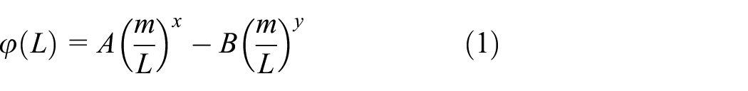
In practical applications, it is often taken as:

Where
Based on the above, the potential function of car-following interaction is established:

Where X is required safety distance.
Differentiating the potential function with respect to the distance can obtain the force and acceleration of the follower:

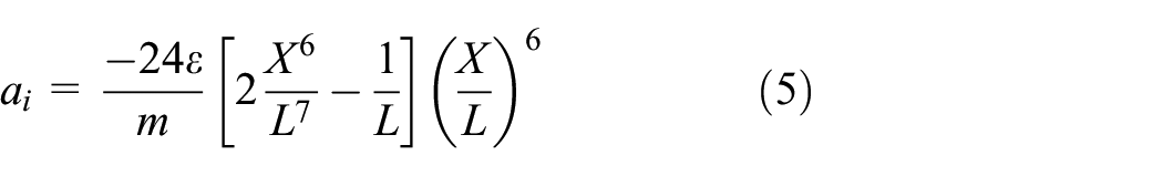
Simplify the model, let

Environmental potential
When a molecule moves in an one-dimensional pipe, it is mainly affected by the interaction potential between molecules and the wall potential, as shown in Figure 3, where

Schematic diagram of wall force.
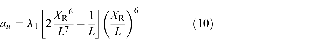
Consistent with molecular dynamics, the environment will also interfere with the behavior of the following car, resulting in an environmental acceleration as
Therefore, the acceleration generated by the following car is:

Some studies 19 have considered that the required safety distance is an instantaneous state quantity, which is the minimum safe braking distance required by the driver from the start of reaction to the stop of car when the car is running at a certain speed. The specific form is:

Where
It can be known from experience that the required safety distance of a car is not only related to the current car’s speed, but also to the speed difference between the front and rear cars. In addition, in order to avoid collision between front and rear cars, there should be an appropriate distance when the car is stopped. So the required safety distance is expressed as:

Where S0 is the distance between two cars when they are stationary; VL is the speed of the leading car; VF is the speed of the following car; amax is the maximum deceleration of the car.
The acceleration generated by the car interaction potential is:
We consider that the state of the leading car is an important environmental stimulus for the following car. Therefore, this paper considers the relative speed of the preceding and following cars, and defines the acceleration caused by the effect of the environment on the following car as:

From the above, the molecular following model is:

Calibration of model parameters
Data collections
The Next Generation Simulation (NGSIM) program 20 is sponsored by the Federal Highway Administration (FHWA) initiated. By setting up a synchronous digital camera network, the researchers collected detailed car trajectory data of US-101 highway in Los Angeles, California, and the southbound direction of Lankershim Avenue, I-80 highway in Emeryville, California, and the eastbound direction of Peachtree Street in Atlanta, Georgia. The time interval of data acquisition is 0.1 s.
In this paper, the detailed trajectory data of cars was used collected from the eastbound direction of I-80 interstate in Emeryville, California. The data was collected by seven cameras installed on the 30 story Pacific Park Plaza building on Christie Avenue, at 10 frames per second. The section of study is 503 m long and divided into six lanes, among which Lane 1 is the High Occupancy car Lanes (HOV) and Lane 6 is the distribution lane, as shown in Figure 4. The I-80 data set includes car trajectory data in three periods, and the road conditions are shown in Table 1.

Outline of the study area.
Road conditions.

In order to ensure the universality of the car-following behavior, the car trajectory data in the period of 4:00 pm–4:15 pm is selected for research. In order to avoid the potential difference of car-following behavior between different types of vehicle, we process the existing data set, extract the car data group with car-following relationship, only study the car-following behavior between small cars, and remove the data from HOV and distribution lane, so as to ensure that the cars studied have similar driving behavior. We use single lane data to avoid the impact of lane change on the following behavior. Based on the above, we finally collected 748575 track records. Each record contains 18 fields, and the complete description is shown in Table 2.
Field descriptions.

Driver’s reaction time
When the driver perceives changes in external information, he needs a certain reaction time to take corresponding actions. Due to the difference in reaction time of drivers, in order to ensure the accuracy of the model, the reaction time of the driver of the following car must be calibrated. Zhang and Bham 21 obtained the reaction time distribution of the following car drivers by studying the car trajectory, as shown in Figure 5. Through calculation, the average response time is 0.396 s, and the standard deviation is 0.109. In this paper, 0.4 s is taken as the reaction time of the follower.
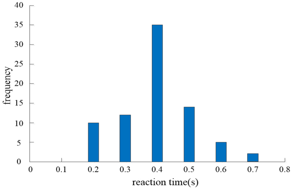
Reaction time distribution map.
Parameter calibration
Due to the different model parameters under different running states of cars, we select 780 groups of car-following data under each state, and use the genetic algorithm described in reference 22 to solve them. The calibration results of molecular car-following model parameters are shown in Table 3.
Model parameter calibration result.

Model evaluation
Numerical simulation of the model
In order to verify the rationality of the molecular car-following model, we choose to compare it with the classical OV model. After decades of development, the OV model has produced many forms, among which the model proposed by Bando et al. 23 is a typical one, and the model expression is:

Where
We use the same data set to calibrate the parameters of the OV model,
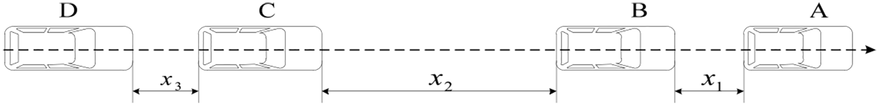
Initial relative position of single lane vehicle following.

Comparison of spatiotemporal trajectories: (a) OV following model, (b) molecular following model, and (c) measured data.
Results and discussion
Figure 7(a) and (b) show the process of the location change caused by the change of the leading vehicle’ speed under different models. It can be seen that there are differences in the reactions of the follower to the leader in different running states. Specifically, as can be seen from Figure 8, for the leader A and the follower B with close headway, the deceleration of B under molecular vehicle following model is more sensitive than that of OV model in the initial 30–40 s deceleration phase. That is to say that follower B decelerates at a higher acceleration, as shown in Figure 8(b). For the leader B and follower C with long distance, the deceleration change of B has less stimulation on C in the molecular vehicle following model than in the OV model, that is, the follower C decelerates with a relatively small acceleration.

Measured speed curve and speed curves under different vehicle following models: (a) OV following model, (b) molecular following model, and (c) measured data.
During the acceleration period between 50 and 70 s in Figure 8(a) and (b), the speed change of vehicle B in the molecular vehicle following model is more gentle than that in the OV following model, it is shown that the vehicle B accelerates and follows with a relatively small acceleration. Comparing the two states of acceleration and deceleration, we can also find that there is an asymmetry in the degree of response of the follower to the acceleration and deceleration. In general, the degree of reaction to long-distance is weaker than that at close range, and the degree of reaction to acceleration is weaker than deceleration.
Under the guidance of the same measured vehicle A, taking the measured acceleration data of measured vehicle B, C, and D as the benchmark, the error between the simulated data and the measured data of the same vehicle under different models is analyzed to compare the reliability of the model in Figure 9. For vehicle B which keeps close following with vehicle A, the absolute value of the maximum acceleration error in MF model is 1.82, while that in OV model is 2.30 (Figure 9(a)). For vehicle C which keeps long distance following with vehicle B, The absolute values of the maximum acceleration error are 2.00 and 1.11 in OV and MF model respectively in Figure 9(b). For vehicle D which keep following with vehicle C at close distance, the maximum acceleration error is 1.51 in OV model, and 1.12 in MF model in Figure 9(c). It can also be seen that in MF model, the error of the simulated is closer to the baseline from the perspective of the whole process, indicating that it is closer to the real situation.
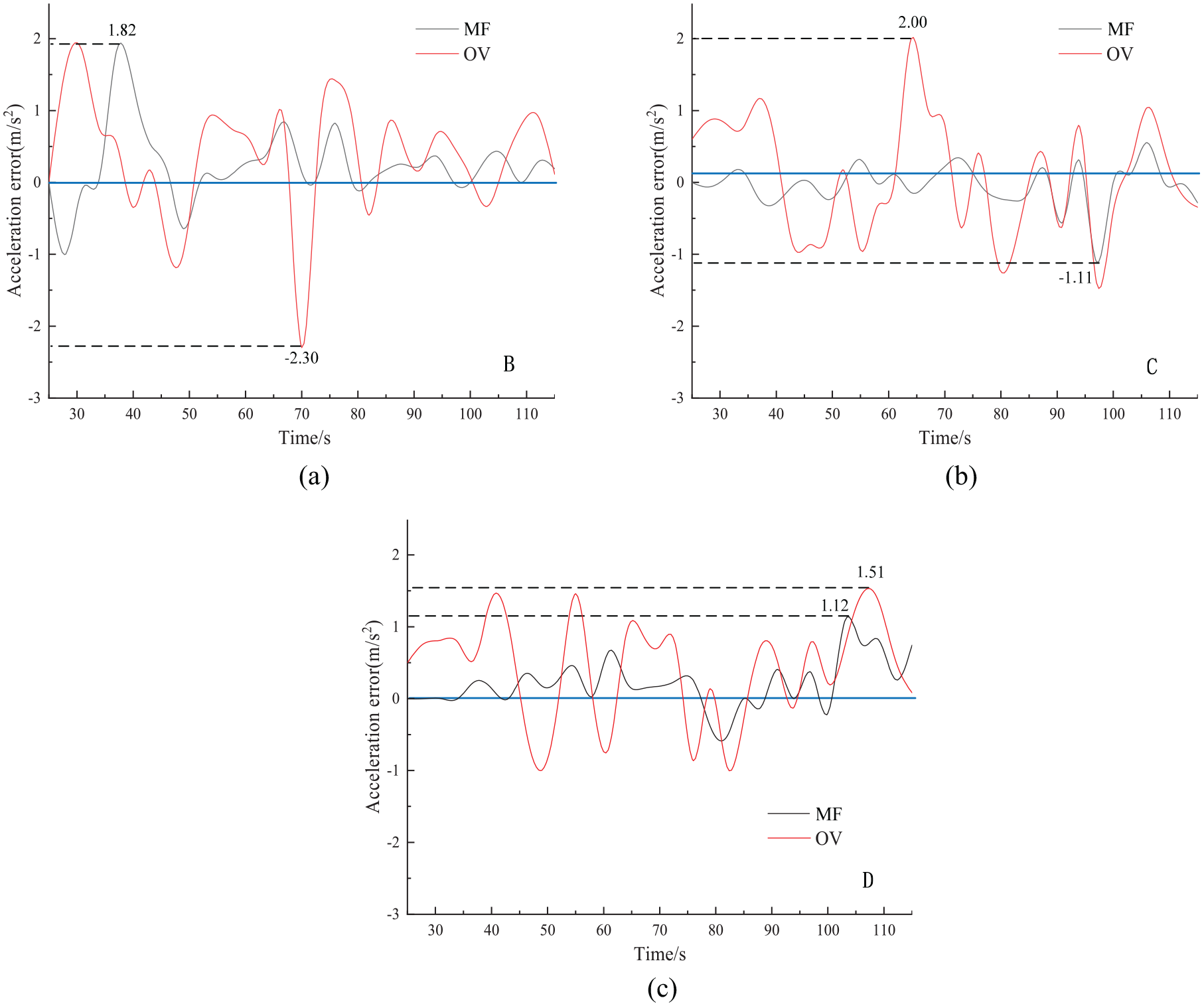
Acceleration error of vehicle B, C and D in two models.
In order to evaluate the model more accurately, we take the mean absolute error (MAE) and root mean square error (RMSE) as the evaluation indexes of the model, and the mathematical expression is as follows:


Where
We substitute the data involved in model parameter calibration into different driving states under the corresponding two models, and the model evaluation results are shown in Table 4 after calculation.
Different model evaluation results.
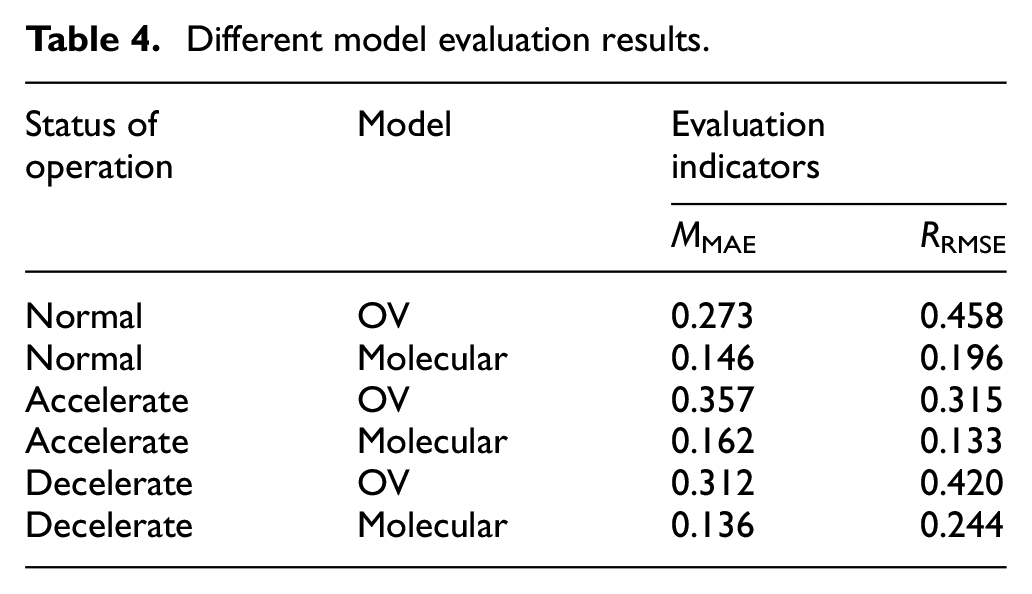
It can be seen from the evaluation results in Table 4 that the mean values of RRMSE and MMAE in the molecular vehicle following model are less than the OV following model, regardless of whether the vehicle is accelerating or decelerating. It proves that the model built can more accurately reflect the vehicle following behavior. The essence can be discussed from the perspective of molecular physical mechanics: (1) When the adjacent vehicle’s distance is gradually smaller than the required safe distance, that is,
Conclusion
The molecular car-following model based on molecular dynamics has higher accuracy and can better explain the driver’s asymmetry in the process of car-following at different distances and in accelerated and decelerated operations. Numerical simulation results show that under the molecular car-following model, the acceleration of the following car during acceleration and deceleration is not constant, but the sensitivity to the deceleration of the leading car is stronger than that during accelerated and decelerated process, and the sensitivity for short-distance acceleration/deceleration is stronger than for long-distance acceleration/deceleration, and the simulation results can be better analyzed from the intermolecular interaction force. The model built can describe the driver’s car-following behavior more closely, so that the following car can better respond to the speed fluctuation of the leading car.
Footnotes
Handling Editor: James Baldwin
Declaration of conflicting interests
The author(s) declared no potential conflicts of interest with respect to the research, authorship, and/or publication of this article.
Funding
The author(s) disclosed receipt of the following financial support for the research, authorship, and/or publication of this article: The authors express their sincere appreciation to the National Natural Science Foundation of China and the Key R & D plan of Shandong Province for the financial support providing under Grants no.51678320 and 2016ZDJ03B01.