Sage Journals: Discover world-class research

Abstract

In this paper, we relax an unrealistic assumption that is commonly adopted in the stability analysis of car-following (CF) models, that is, the equilibrium state is fixed. Specifically, the influence mechanism of the equilibrium state and equilibrium state change on the stability of CF models is studied considering the impact of asymmetry in CF models. Two state change processes are considered: acceleration and deceleration processes for symmetric and asymmetric CF models. The results reveal that significant differences exist between the two types of CF models: while the acceleration process would significantly destabilize the traffic with the asymmetric CF model, the influence of acceleration and deceleration on its stability change is identical and relatively unsignificant for the symmetric CF model.

Keywords

operations car following models simulation traffic flow

The stability of car-following (CF) models has been studied for almost 60 years, since the early days of CF model development ( 1 ), with respect to a small perturbation’s evolution over time (i.e., local stability) and over a platoon (i.e., string stability). Several theoretical methods have been proposed for the local and string stability analysis of different types of CF models, and they were reviewed and compared in detail in our previous paper ( 2 ). More details are provided in the Literature Review section. Because local stability can be easily achieved for most CF models, string stability is the concern of this paper. From here on, stability analysis means string stability analysis unless stated otherwise.

In conventional stability analysis, a key assumption is that the equilibrium state is fixed. In other words, a driver who deviated from the equilibrium state always returns to the same equilibrium state without changing speed or spacing after having experienced a perturbation. However, this contradicts with observations in real traffic, where drivers are more likely to converge to different equilibrium states in different traffic conditions. Furthermore, as revealed in the recent literature ( 3 , 4 ), experiencing perturbations itself can change how a driver behaves. Therefore, to enhance the practical value of the stability analysis of CF models, dynamic equilibrium states, rather than a fixed equilibrium state, should be considered to represent real traffic more realistically.

Generally, equilibrium speed, spacing, or both, play different roles in the string stability criteria of different CF models ( 5 ). For different CF models, when dynamic equilibrium states are considered their stability characteristics can be distinctively different. For instance, the stability criteria of intelligent driver model (IDM [ 6 ]) and Gipps’ model ( 7 ) are dependent of the equilibrium speed and spacing, while the stability criteria of the optimal velocity model (OVM [ 8 ]) and its extension the full velocity difference model (FVDM [ 9 ]) with a specific optimal velocity (OV) function are not influenced by either speed or spacing. Therefore, the stability of some CF models (e.g., the IDM) naturally varies with traffic states, while the stability of others does not.

Furthermore, drivers can behave differently in different states. For example, drivers usually are more attentive in deceleration compared with their behavior in acceleration. Such asymmetric behavior is believed to be a main cause that triggers the widely reported traffic hysteresis phenomenon ( 10 – 13 ), which is considered in some CF models (e.g., the IDM, Gipps’ model) while it is ignored in many (e.g., the OVM, FVDM). Thus, when the fixed equilibrium state assumption is relaxed, a natural question that deserves in-depth investigation is: how does the disturbance propagate differently along the platoon during the acceleration and deceleration processes between a symmetric CF model and an asymmetric one?

The objective of this paper is thus to understand the mechanism of the stability evolution of different CF models with dynamic equilibrium states. Using the IDM and OVM as examples, we first examine the impact of various equilibrium states on different CF models’ stability. After that, considering the existence of diverse CF regimes (e.g., the acceleration and deceleration regimes), we further investigate dynamic equilibrium states’ influence on CF models’ stability, and reveal and compare the stability evolution characteristics of symmetric and asymmetric CF models that go through dynamic equilibrium states.

The remainder of this paper is organized as follows: the next section introduces the string stability and related studies; the third section studies the impact of the dynamic equilibrium state on CF models’ stability; the fourth section investigates CF models’ stability evolution characteristics under traffic state change conditions; and the fifth section summarizes and discusses the main findings of this study.

Literature Review

For a homogenous vehicular platoon, if the perturbation originating from the first vehicle strictly decreases along the platoon, the platoon is string stable; otherwise, it is string unstable. As mentioned in the first section, several notable methods have been adopted to analyze the string stability for different types of analytical CF models (i.e., basic, time-delayed, and multi-anticipative/cooperative CF models) ( 2 ), that is, characteristic equation-based, direct transfer function-based, and Laplace transform-based methods. The characteristic equation-based method is a general method in stability analysis, which is based on the characteristic equation induced from linearized CF models with the use of exponential ansatz to represent perturbations, and is widely used in the literature (5, 14 –21). The direct transfer function-based method calculates the magnitude of the transfer function with the Fourier ansatz ( 1 , 22 ), while the Laplace transform-based method uses the Laplace transform to calculate the magnitude of the transfer function in the frequency domain (17, 19, 23 –28). The mathematical details of these methods are provided by Sun et al. ( 2 ).

In addition, for the convenience of theoretical analysis, the conventional stability analysis of CF models usually adopts several assumptions that are not realistic in real traffic, for example, fixed equilibrium state, homogeneous platoon (vehicles are identical), infinite-size platoon (the number of vehicles in the platoon is arbitrarily large), and long-wavelength perturbation (the wavelength of the first unstable perturbation tends to infinity). Recently, these assumptions have been partially relaxed in different ways. Specifically, several studies have focused on the heterogeneous platoon (15, 29 –31). Sun et al. ( 32 ) developed the quantitative relationship between CF string instability and traffic oscillation by relaxing the infinitely long platoon and long-wavelength perturbation assumption. The stochasticity within CF models was also considered in string stability analysis ( 33 ). However, the impact of the fixed equilibrium state on the stability evolution is not reported in the literature, which is the primary motivation of this study.

Impact of the Equilibrium State on Car-Following Models’ Stability

For the convenience of discussion, we consider a typical scenario of CF, where identical vehicles with length l are traveling in a single lane without overtaking. Vehicle n follows vehicle (n–1); $x_{n}$ and $x_{n - 1}$ denote the position of the nth and (n–1)th vehicles, respectively; $v_{n}$ and $v_{n - 1}$ denote the speed of the nth and (n–1)th vehicles, respectively; $s_{n} = x_{n - 1} - x_{n} - l$ is the gap between these two vehicles (the rear bumper of the (n–1)th vehicle to the front bumper of the nth vehicle); $Δ v_{n} (t) = v_{n - 1} (t) - v_{n} (t)$ is the relative speed of vehicle n with the leading vehicle (n–1). In a steady state, all vehicles travel at the same speed $v_{e}$ with the same gap $s_{e}$ .

The IDM developed by Treiber et al. ( 6 ) and the OVM developed by Bando et al. ( 8 ) are used in this study mainly for two reasons: (i) they represent different types of CF models, as the IDM is asymmetric while the OVM is symmetric; and (ii) their stability has been widely analyzed in the literature ( 5 , 15 , 16 ).

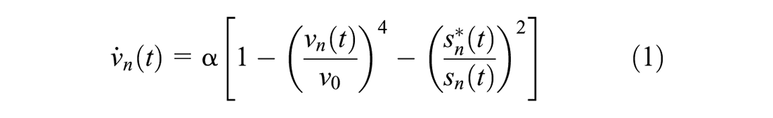
The IDM is mathematically formulated as in Equations 1 and 2:

{\overset{\cdot}{v}}_{n} (t) = α [1 - {(\frac{v_{n} (t)}{v_{0}})}^{4} - {(\frac{s_{n}^{*} (t)}{s_{n} (t)})}^{2}]

(1)

s_{n}^{*} (t) = s_{0} + T v_{n} (t) - \frac{v_{n} (t) Δ v_{n} (t)}{2 \sqrt{α β}}

(2)

where $v_{0}$ is the desired speed, $s_{n}^{*} (t)$ is the desired gap, $s_{0}$ is the minimum gap in the standstill situation, T is the desired time gap, α is the maximum acceleration, and β is the comfortable deceleration.

For the OVM, its basic form is ${\overset{\cdot}{v}}_{n} (t) = k [v_{o p t} (s) - v_{n} (t)]$ , where k is the sensitivity parameter and $v_{o p t} (s)$ is the OV function with respect to spacing $s_{n}$ . The original OV function in Bando et al. ( 8 ) uses a hyperbolic tangent. To be consistent with the analysis of the IDM, a more intuitive OV function presented by Treiber and Kesting ( 5 ) is adopted in this study, as shown in Equation 3:

v_{o p t} (s) = max [0, \min (v_{0}, \frac{s_{n} (t) - s_{0}}{T})]

(3)

where the variables have the same meanings as introduced before.

According to ( 2 , 23 , 34 ), there exists a general string stability criterion for basic CF models (without considering any time delays), as shown in Equation 4:

\frac{1}{2} - \frac{f_{Δ v}}{f_{v}} - \frac{f_{s}}{f_{v}^{2}} > 0

(4)

where $f_{s} = \frac{\partial f}{\partial s} |_{e}, f_{v} = \frac{\partial f}{\partial v} |_{e}, f_{Δ v} = \frac{\partial f}{\partial Δ v} |_{e}$ are the Taylor expansion coefficients of the acceleration function in the steady state with respect to different variables after first-order linearization.

This string stability criterion is applied to the IDM and OVM, respectively. For the IDM, its stability criterion can be constructed using its Taylor expansion coefficients, as shown in Equations 5 –7:

f_{s} = \frac{2 α}{s_{e}} {(\frac{s_{0} + T v_{e}}{s_{e}})}^{2}

(5)

f_{v} = - α [\frac{4}{v_{0}} {(\frac{v_{e}}{v_{0}})}^{3} + \frac{2 T (s_{0} + T v_{e})}{{s_{e}}^{2}}]

(6)

f_{Δ v} = \sqrt{\frac{α}{β}} \frac{v_{e}}{s_{e}} \frac{s_{0} + T v_{e}}{s_{e}}

(7)

The stability criterion of the OVM is simply $k > \frac{2}{T}$ .

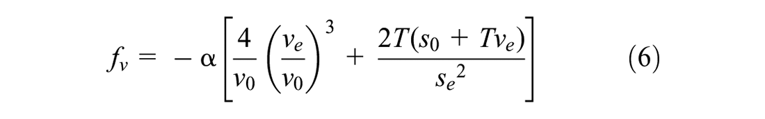
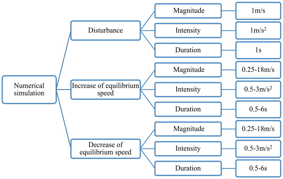
From the stability criteria of the IDM and OVM, we can clearly see that the stability of the IDM varies with different traffic states (measured by the equilibrium speed $v_{e}$ or the equilibrium gap $s_{e})$ , while that of the OVM has nothing to do with either $v_{e}$ or $s_{e}$ .

To further assess the influence of traffic states on stability, the string stability region defined by the desired time gap T and maximum acceleration α in the IDM (the desired time gap T and sensitivity parameter k in the OVM) is plotted with different equilibrium speeds, as shown in Figure 1. This figure reveals that the stability region of the IDM changes significantly as the equilibrium speed changes from 2 to 20 m/s. The stability region of the OVM is unchanged for equilibrium speeds, since the stability criterion is independent of the speed.

Figure 1.

The stability region of (a) the intelligent driver model and (b) optimal velocity model with various equilibrium speeds (other parameters are default: desired speed $v_{0} =$ 120 km/h; comfortable deceleration β = 1.5 m/s²; minimum gap $s_{0} =$ 2 m; vehicle length l = 5 m).

As we can see from Figure 1a, with the increase of equilibrium speed, the stability of the IDM becomes greater when the maximum acceleration is larger than 1 m/s², while it tends to be more unstable when the maximum acceleration is less than 1 m/s². Similar results can be found with respect to different desired time gaps: the increase of equilibrium speed improves the IDM’s stability when the desired time gap is under 1.2 s, and deteriorates the IDM’s stability when the desired time gap is above 1.2 s. For typical IDM parameters for reproducing real traffic where the maximum acceleration is larger than 1 m/s² and the desired time gap is less than 1.2 s ( 5 , 32 , 35 ), its stability will be enhanced with better traffic conditions (e.g., a higher equilibrium speed).

Impact of the Traffic State Change on Car-Following Models’ Stability

In real-world traffic, drivers frequently experience traffic state changes. Consequently, drivers need to decelerate or accelerate to adapt to changing traffic states. It is widely acknowledged that while drivers are going through traffic state changes, their behavior in the acceleration process is usually different from their behavior in the deceleration process ( 11 , 13 , 36 ). Such a behavioral asymmetry leads to the traffic hysteresis phenomenon. As shown in the previous section, different equilibrium states lead to different stability regions of the IDM model. What is not clear is whether and how much traffic state changes affect the stability evolution of CF models. This is an important question that can help us to understand the practical value of the stability analysis. To this end, we select the IDM as a representative of asymmetric CF models and the OVM as a representative of symmetric CF models to investigate their stability evolutions as the traffic state changes. Because the traffic state change is not considered in the theoretical stability analysis of CF, numerical simulation is a convenient yet effective way to investigate dynamic equilibrium states’ influence on CF models’ stability by simulating a platoon of vehicles that move on a single-lane straight road. Then the string stability can be decided based on how the disturbance evolves along the platoon.

Simulation Setup

Similar to the simulation setup in Sun et al. ( 2 ), vehicles in the platoon quickly reach the equilibrium state and then travel with the same speed and the corresponding equilibrium gap. At t = 60 s, a disturbance is introduced to the first leading vehicle by forcing it to first decelerate (accelerate) and then accelerate (decelerate) for the same time duration. However, unlike studies in the literature, after experiencing the disturbance the first vehicle does not return to the original equilibrium state, but rather converges to a different equilibrium state, which guarantees the occurrence of a traffic state change. Two typical state change processes are considered separately in two cases as described below.

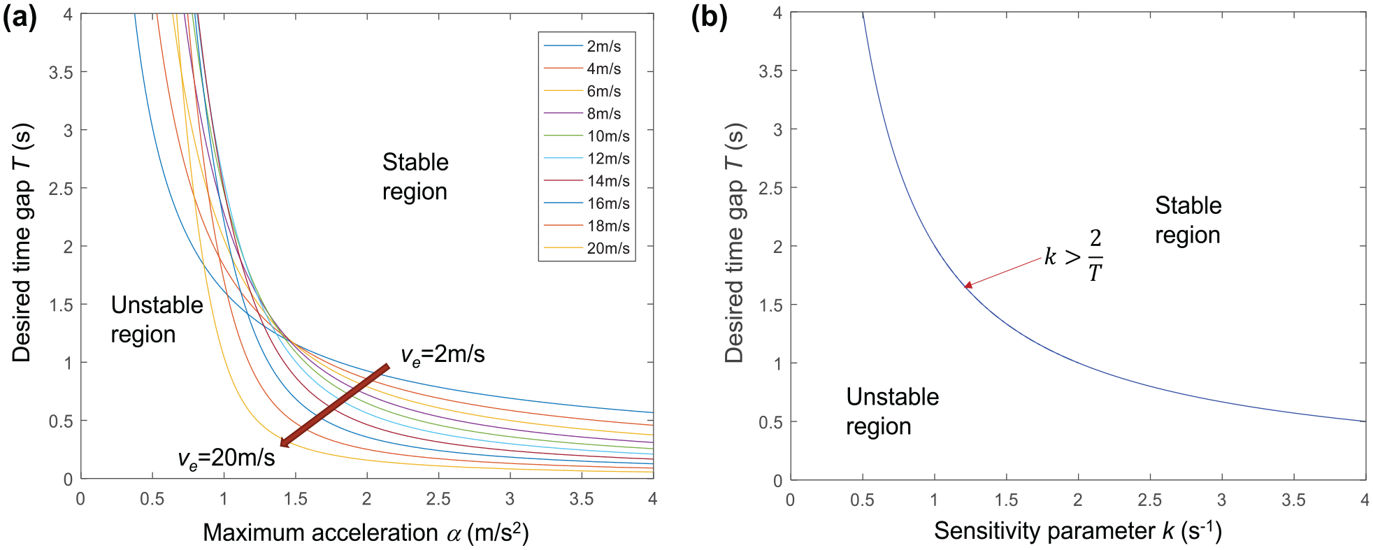
Case I: the first leading vehicle travels at the equilibrium speed of 10 m/s. After experiencing the disturbance, the first leading vehicle accelerates until a higher equilibrium speed (i.e., 15 m/s) is reached.

Case II: the first leading vehicle travels at the equilibrium speed of 10 m/s. After experiencing the disturbance, the first leading vehicle decelerates until a lower equilibrium speed (i.e., 5 m/s) is reached.

The speed profile of the first leading vehicle in each case is shown in Figure 2. In both cases, the magnitude of equilibrium speed change is the same (i.e., 5 m/s).

Figure 2.

The speed profiles of the first vehicle in the simulations (the magnitude of equilibrium speed change is 5 m/s: the first accelerates/decelerates with 1 m/s² for 5 s after a disturbance): (a) accelerating after a disturbance and (b) decelerating after a disturbance.

Although the change in equilibrium speed can be considered as another type of disturbance to the following vehicles, here, we mainly focus on the evolution of the first small disturbance introduced to the leading vehicle before the equilibrium speed change following the string stability definition. The speed deviations of vehicles from the equilibrium speed (no matter whether and how the equilibrium speed changes) in the platoon are measured for determining the string stability: if the absolute speed deviation of all the following vehicles strictly decreases along the platoon, the platoon is string stable; otherwise, it is string unstable.

As per Sun et al. ( 2 ), to obtain a reliable result for stability analysis, the platoon size is set as 100 vehicles. In each simulation step, the following vehicles move forward by calculating the acceleration according to the IDM or OVM, while the speed and position of the vehicles are updated with the trapezoidal rule, as shown in Equations 8 and 9 ( 37 ). Note that all the numerical simulations are programmed in MATLAB:

v_{n} (t + Δ T) = v_{n} (t) + \frac{1}{2} (a_{n} (t) + a_{n} (t + Δ T)) Δ T

(8)

x_{n} (t + Δ T) = x_{n} (t) + v_{n} (t) Δ T + \frac{a_{n} (t) {(Δ T)}^{2}}{2}

(9)

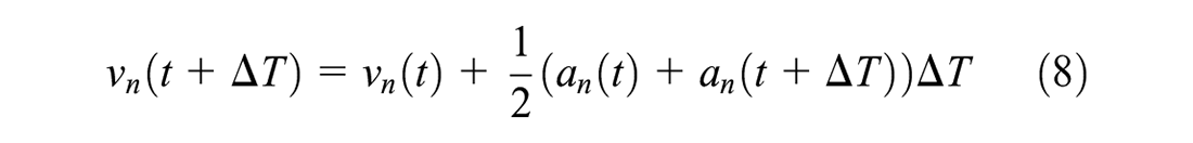
where $Δ T$ is the update time step, which is set as 0.1 s in our simulations.

To rigorously evaluate the influence of the state change on stability, several main factors that may affect the results are considered:

the original equilibrium speed (e.g., 5, 10, 15, and 20 m/s);

the intensity of the state change (measured by the acceleration rate, and the range considered is 0.5–3 m/s²);

the duration of the state change (measured by acceleration/deceleration time, and the range considered is 0.5–6 s);

and the magnitude of state change (measured by the product of the intensity and duration, i.e., the total amount of the equilibrium speed change).

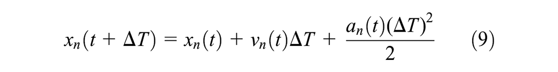
The ranges of these factors are chosen by considering two goals: (1) to keep the values realistic (e.g., the real acceleration/deceleration should be not lager than 3 m/s²); and (2) to generate many diverse test scenarios (e.g., the equilibrium speed can be decreased from 20 to 2 m/s). Without loss of generality, the magnitude of the disturbance is fixed at 1 m/s, which is realized by making the first vehicle decelerate (accelerate) with 1 m/s² for 1 s and then accelerate (decelerate) with 1 m/s² for 1 s before accelerating (decelerating) to another equilibrium speed. The setup of numerical simulation is summarized in Figure 3.

Figure 3.

Setup of the numerical simulation for speed change analysis.

Results for the IDM

Some 1600 combinations of different parameters of the IDM are simulated. More specifically, the main factors considered are the desired time gap T (0.1–4 s) and the maximum acceleration α (0.1–4 m/s²). Other parameters of the IDM are default: desired speed $v_{0} =$ 120 km/h; comfortable deceleration β = 1.5 m/s²; minimum gap $s_{0} =$ 2 m; and vehicle length l = 5 m. For each simulation run, the platoon’s stability is assessed using the definition of string stability.

Based on the stability assessment results for all the simulation runs, we plot the stability region of the IDM when traffic state changes, as shown in Figure 4. Figure 4a is for Case I where drivers accelerate to a higher equilibrium speed; Figure 4b is for Case II where drivers decelerate to a lower equilibrium speed. In each figure, dots represent the simulation runs in which the platoon was string unstable, while the blank area represents the simulation runs in which the platoon was string stable. Then, the stability region with the traffic state change (derived from the simulation results) is compared with the theoretical results without the traffic state change.

Figure 4.

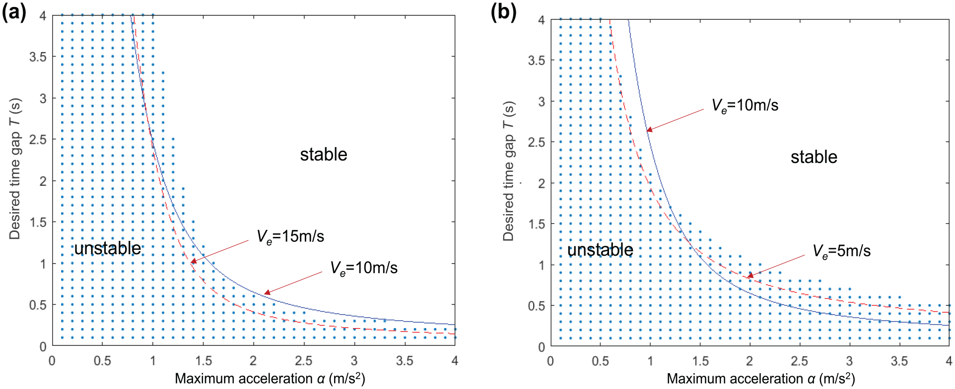
Stability regions for different scenarios: (a) string stability region for the intelligent driver model (IDM) (the solid curve denotes the boundary between the theoretical stable area and the unstable area for the original equilibrium speed $v_{e}$ = 10 m/s and the dashed curve denotes the boundary for the increased equilibrium speed $v_{e}$ = 15 m/s; the points denote the string unstable parameter sets from simulation; the magnitude of the speed change in this scenario is 5 m/s: the first vehicle accelerates with 1 m/s² for 5 s after experiencing the disturbance, as shown in Figure 2a); (b) string stability region for the IDM (the solid curve denotes the boundary between the theoretical stable area and the unstable area for the original equilibrium speed $v_{e}$ = 10 m/s and the dashed curve denotes the boundary for the decreased equilibrium speed $v_{e}$ = 5 m/s; the points denote the string unstable parameter sets from simulation; the magnitude of the disturbance in this scenario is 5 m/s: the first vehicle decelerates with 1 m/s² for 5 s after experiencing the disturbance, as shown in Figure 2b).

In Figure 4a, the solid curve is the boundary between the theoretical stable area and the unstable area for the original traffic state at the equilibrium speed $v_{e}$ = 10 m/s, and the dashed curve is the boundary for the new traffic state at the equilibrium speed $v_{e}$ = 15 m/s. This figure clearly shows that compared with the cases where traffic stays in the same equilibrium state, the traffic state change via the acceleration process increases the traffic instability because the unstable area from the simulation result is larger than either that for the original equilibrium speed or that for the new equilibrium speed.

In Figure 4b, the solid curve is the boundary between the theoretical stable area and the unstable area for the original traffic state at the equilibrium speed $v_{e}$ = 10 m/s, and the dashed curve is the boundary for the new traffic state at the equilibrium speed $v_{e}$ = 5 m/s. Similarly, this figure shows that traffic state change via the deceleration process also increases the traffic instability, albeit to a lesser extent. In addition, Figure 4 shows that the acceleration process makes the system more unstable in the lower range of the maximum acceleration (0–1.5 m/s² approximately), while the opposite is observed for the deceleration process, that is, the deceleration process makes the system more unstable in the higher range of the maximum acceleration (1.5–4 approximately m/s²).

Another interesting observation from Figure 4 is that when traffic accelerates from one equilibrium state to a new equilibrium state (Case I), for the higher range of maximum acceleration the stability boundary of the traffic can be well approximated by using the theoretical stability boundary for the state of the lower equilibrium speed (i.e., the state before the acceleration), while for the lower range of maximum acceleration the stability boundary of the traffic cannot be well approximated by using the theoretical stability boundary either for the state of the lower equilibrium speed or for the state of the higher equilibrium speed, as both would notably underestimate the unstable area; when traffic decelerates from one equilibrium state to a new equilibrium state (Case II), the opposite trend exists. More specifically, for the lower range of maximum acceleration the stability boundary of the traffic can be well approximated by using the theoretical stability boundary for the state of the lower equilibrium speed (i.e., the state after the deceleration), while for the higher range of maximum acceleration the stability boundary of the traffic cannot be well approximated by using the theoretical stability boundary either for the state of the lower equilibrium speed or for the state of the higher equilibrium speed, as both would notably underestimate the unstable area.

Next, the percentage of the unstable area over the whole stability region is adopted to quantify the stability change. The impact of equilibrium speed change on the stability of the IDM is shown in Figure 5, where the dots denote the theoretical results of unstable area percentages from the conventional stability analysis (i.e., without equilibrium speed change) over different equilibrium speeds, while other markers indicate unstable area percentages from the simulation results when the traffic state changes from different original equilibrium speeds to new higher (Figure 5a) or lower (Figure 5b) equilibrium speeds. The horizontal axis is the new equilibrium speed after accelerating/decelerating from the original one.

Figure 5.

The impact of equilibrium speed change on the percentage of unstable area for the intelligent driver model: (a) increase of equilibrium speed and (b) the decrease of equilibrium speed.

As shown in Figure 5, with the increase of equilibrium speed the instability of the IDM first increases and then decreases. However, the stability of the IDM without the state change is always higher than that at the changed equilibrium speed. Moreover, in the deceleration scenarios, as shown in Figure 5b, the instability trend of the IDM over the equilibrium speed decrease is consistent with the trend of the theoretical instability change over different equilibrium speeds, while as shown in Figure 5a, in the acceleration scenarios the instability trend over the equilibrium speed increase is only consistent with the trend of the theoretical instability change over a small range (about 3 m/s), and then the instability percentages increase significantly as the equilibrium speed keeps increasing. However, once the increased equilibrium speed is sufficiently large, the instability percentage becomes no longer sensitive to the change of equilibrium speed. Figure 5, a and b , also clearly depicts that, for the IDM, as an asymmetric CF model, the trend of its instability change in the acceleration process differs from that in the deceleration process. More specifically, compared with the deceleration process, the acceleration process deteriorates more of the IDM’s ability of compressing a perturbation’s propagation along a platoon.

Results for the OVM

Similar to the simulation for the IDM, 1600 combinations of the parameter set (desired time gap T (0.1–4 s) and sensitivity parameter k [0.1–4 s⁻¹]) are simulated for the OVM. Other parameters for the OVM are default: desired speed $v_{0} =$ 120 km/h; minimum gap $s_{0} =$ 2 m; and vehicle length l = 5 m. The string stability region for the OVM defined by the desired time gap T and sensitivity parameter k is also plotted when the traffic state changes. Figure 6 shows one example, where the equilibrium speed increases from 10 to 15 m/s, as the first vehicle of the platoon goes through the speed profiles, shown in Figure 2a. The solid curve in Figure 6 denotes the boundary between the theoretical stable area and the unstable area. Note that unlike for the IDM where two curves/boundaries exist from the theoretical stability analysis (see Figure 4), only one theoretical boundary is obtained for the OVM despite the first vehicle experiencing the same traffic state changes. This is because, as mentioned before, the stability criterion of the OVM is independent of the equilibrium speed/gap; thus, the stability boundary of the OVM is not influenced by the traffic state changes. The dots in Figure 6 denote the string unstable parameter sets from the simulation. As expected, like what we have observed for the IDM, the acceleration process increases the instability of the OVM. Note that the deceleration process (in which the equilibrium speed decreases from 10 to 5 m/s) gives the same result. To save space, the figure for the deceleration process is not repeated here.

Figure 6.

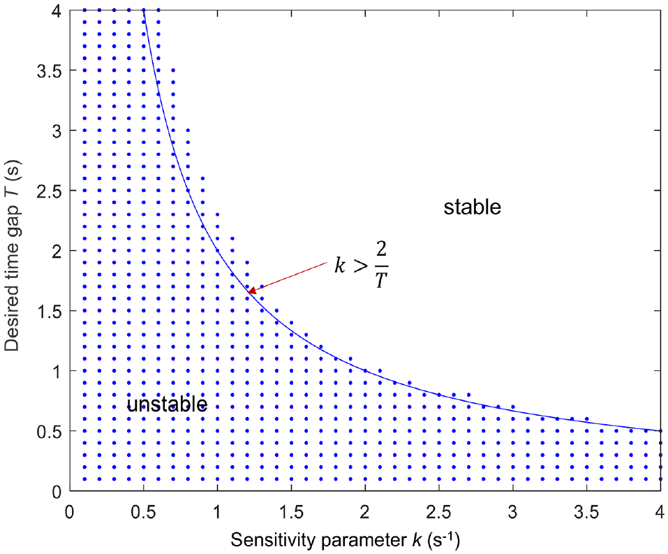
String stability region for the optimal velocity model (the solid curve denotes the boundary between the theoretical stable area and the unstable area [independent of the equilibrium speed]; the dots denote the string unstable parameter sets from simulation; the magnitude of the disturbance in this scenario is 5 m/s: the first vehicle accelerates with 1 m/s² for 5 s after experiencing the disturbance, as shown in Figure 2a).

Similarly, the percentage of the unstable area over the whole stability region is adopted to quantify the stability change, and result is shown in Figure 7. In this figure, the theoretical results from the conventional stability analysis (i.e., without equilibrium speed change) are indicated by the dots, while other markers indicate the simulation results with the state changes from different original equilibrium speeds to various new equilibrium speeds. Again, because of the independence of equilibrium speed in the conventional stability analysis of the OVM, the percentage of unstable area in the conventional stability analysis remain constant across different equilibrium speeds. The same as the IDM, the instability of the OVM becomes amplified during the acceleration/deceleration process, where a larger speed change always leads to a larger unstable region. In addition, for the OVM, as a symmetric CF model, the influence of acceleration and deceleration on the OVM’s stability change is identical, and also different original equilibrium speeds have no impact, which is clear by comparing Figure 7a with Figure 7b.

Figure 7.

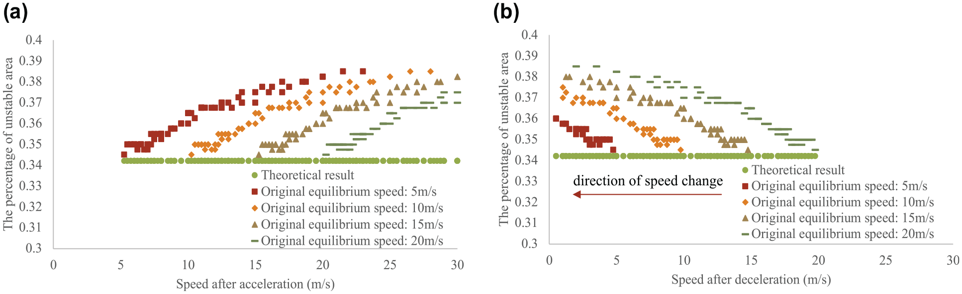
The impact of equilibrium speed change on the percentage of unstable area for the optimal velocity model: (a) increase of equilibrium speed and (b) decrease of equilibrium speed.

To quantitively compare the impact of dynamic equilibrium speeds on the stability of different CF models, we further calculate the average increased percentage of the unstable area of the equilibrium speed change between 5, 10, 15, and 20 m/s, with the results presented in Table 1. Consistent with the conclusions drawn before, the results clearly show the more significant negative impact of the equilibrium speed change for the IDM compared to the OVM, especially with the equilibrium speed increased at the acceleration process. The stability decreases slightly (from 0.021 to 0.041) with a larger speed change, while the change in amplitude remains the same with the same speed change (no matter the acceleration or deceleration) for the OVM. For the IDM, the stability deteriorates significantly with the increase of speed (from 0.075 to 0.299) and it has a much slighter change with the decrease of speed (from 0.034 to 0.065).

Table 1.

The Average Increased Percentage of the Unstable Area Between Different Equilibrium Speeds for the Intelligent Driver Model/Optimal Velocity Model

Original speed	Changed speed
Original speed	5 m/s	10 m/s	15 m/s	20 m/s
5 m/s	0	0.085/0.021	0.194/0.031	0.299/0.041
10 m/s	0.039/0.021	0	0.078/0.021	0.209/0.031
15 m/s	0.045/0.031	0.048/0.021	0	0.075/0.021
20 m/s	0.065/0.041	0.063/0.031	0.034/0.021	0

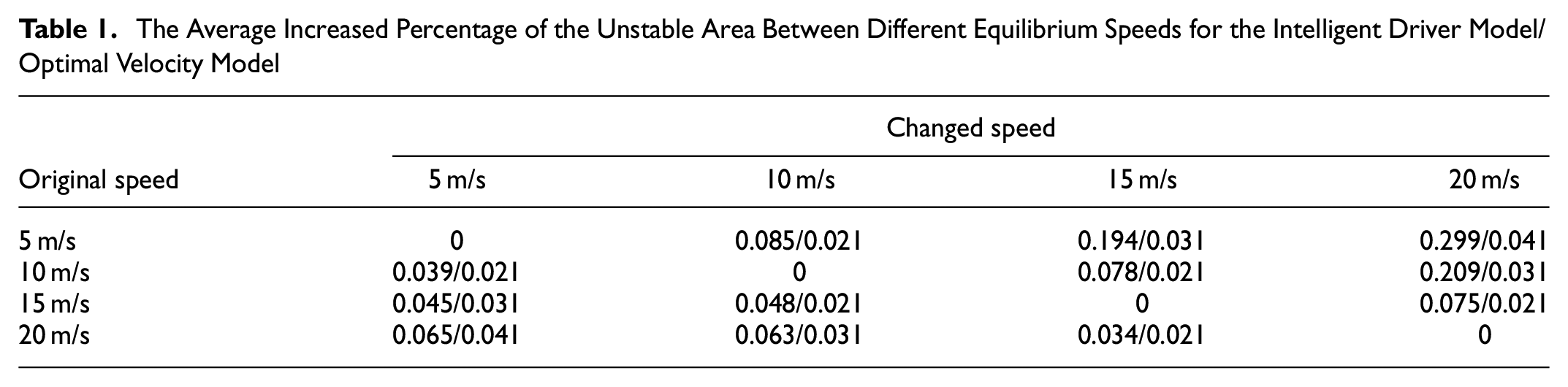
We then can conclude that the asymmetry of CF models has a significant impact on the stability change within dynamic equilibrium traffic flow, while the stability of symmetric CF models is steadier during the state change process. Although it has been proved that asymmetric CF models can depict real traffic more accurately ( 38 ), such steady characteristics of symmetric CF models can have important implications for developing driving strategies for automated vehicles, as we will be less likely to confront instability growth after assigning appropriate parameters, especially during the acceleration process.

Conclusions

Because one important assumption adopted in traditional stability analysis is that traffic returns to the same equilibrium state after having experienced a small disturbance, which makes it incompatible with traffic oscillations observed in traffic congestion, and consequently makes it generally difficult to directly use these stability criteria in designing traffic operation and control strategies, this paper aims to investigate the stability evolution of CF models under dynamic equilibrium states. Furthermore, the impact of the equilibrium state change is scrutinized by considering two driving regimes for two types (symmetric and asymmetric) of CF models: the acceleration and deceleration processes. To demonstrate the differences between these two types of CF models, the OVM and IDM are used in this paper as a representative of each type.

Significant differences between the two CF models are found for the stability change with different equilibrium speeds. The stability of the IDM changes with different traffic states, while that of the OVM is constant. Moreover, the mechanisms of stability evolution of the IDM and OVM when the equilibrium state changes have been obtained. From the huge number of simulations, we have found that the stability of both the IDM and OVM always decreases when the equilibrium state changes, compared with their stability at the original equilibrium speed. However, there are subtle but important differences between these two models. For the IDM, as an asymmetric CF model, the trend of stability change in the acceleration process differs from that in the deceleration process. More specifically, the acceleration process would significantly destabilize the traffic. For the OVM, as a symmetric CF model, the influence of acceleration and deceleration on its stability change is identical, while different original equilibrium speeds make no difference. Such steady characteristics of symmetric CF models could facilitate developing driving strategies for automated vehicles, as we do not need to worry much about its stability variation in different driving regimes, whereas the acceleration part of an asymmetric CF model may need to be adapted for more stable traffic.

Footnotes

Author Contributions

The authors confirm contribution to the paper as follows: study conception and design: Jie Sun, Z. Zheng; data collection: Jie Sun; analysis and interpretation of results: Jie Sun, Z. Zheng, Jian Sun; draft manuscript preparation: Jie Sun, Z. Zheng. All authors reviewed the results and approved the final version of the manuscript.

Declaration of Conflicting Interests

The author(s) declared no potential conflicts of interest with respect to the research, authorship, and/or publication of this article.

Funding

The author(s) disclosed receipt of the following financial support for the research, authorship, and/or publication of this article: This research was partially funded by the Australian Research Council (ARC) (DP210102970).

ORCID iDs

Jie Sun

Zuduo Zheng

Jian Sun

References

Chandler

R. E.

Herman

Montroll

E. W.

Traffic Dynamics: Studies in Car Following. Operations Research, Vol. 6, No. 2, 1958, pp. 165–184.

Sun

Zheng

Sun

Stability Analysis Methods and Their Applicability to Car-Following Models in Conventional and Connected Environments. Transportation Research Part B: Methodological, Vol. 109, 2018, pp. 212–237.

Zheng

Ahn

Chen

Laval

Freeway Traffic Oscillations: Microscopic Analysis of Formations and Propagations Using Wavelet Transform. Transportation Research Part B: Methodological, Vol. 45, No. 9, 2011, pp. 1378–1388.

Zheng

Ahn

Chen

Laval

The Effects of Lane-Changing on the Immediate Follower: Anticipation, Relaxation, and Change in Driver Characteristics. Transportation Research Part C: Emerging Technologies, Vol. 26, 2013, pp. 367–379.

Treiber

Kesting

Traffic Flow Dynamics: Data, Models and Simulation. Springer-Verlag, Berlin Heidelberg, 2013.

Treiber

Hennecke

Helbing

Congested Traffic States in Empirical Observations and Microscopic Simulations. Physical Review E, Vol. 62, No. 2, 2000, p. 1805.

Gipps

P. G.

A Behavioural Car-Following Model for Computer Simulation. Transportation Research Part B: Methodological, Vol. 15, No. 2, 1981, pp. 105–111.

Bando

Hasebe

Nakayama

Shibata

Sugiyama

Dynamical Model of Traffic Congestion and Numerical Simulation. Physical Review E, Vol. 51, No. 2, 1995, p. 1035.

Jiang

Zhu

Full Velocity Difference Model for a Car-Following Theory. Physical Review E, Vol. 64, 2001, p. 017101.

10.

Zhang

H. M.

A Mathematical Theory of Traffic Hysteresis. Transportation Research Part B: Methodological, Vol. 33, No. 1, 1999, pp. 1–23.

11.

Saifuzzaman

Zheng

Haque

M. M.

Washington

Understanding the Mechanism of Traffic Hysteresis and Traffic Oscillations Through the Change in Task Difficulty Level. Transportation Research Part B: Methodological, Vol. 105, 2017, pp. 523–538.

12.

Laval

J. A.

Hysteresis in Traffic Flow Revisited: An Improved Measurement Method. Transportation Research Part B: Methodological, Vol. 45, No. 2, 2011, pp. 385–391.

13.

Chen

Laval

J. A.

Ahn

Zheng

Microscopic Traffic Hysteresis in Traffic Oscillations: A Behavioral Perspective. Transportation Research Part B: Methodological, Vol. 46, No. 10, 2012, pp. 1440–1453.

14.

Monteil

Billot

El Faouzi

N.-E.

Linear and Weakly Nonlinear Stability Analyses of Cooperative Car-Following Models. IEEE Transactions on Intelligent Transportation Systems, Vol. 15, No. 5, 2014, pp. 2001–2013.

15.

Ngoduy

Analytical Studies on the Instabilities of Heterogeneous Intelligent Traffic Flow. Communications in Nonlinear Science and Numerical Simulation, Vol. 18, No. 10, 2013, pp. 2699–2706.

16.

Ngoduy

Linear Stability of a Generalized Multi-Anticipative Car Following Model With Time Delays. Communications in Nonlinear Science and Numerical Simulation, Vol. 22, 2015, pp. 420–426.

17.

Orosz

Moehlis

Bullo

Delayed Car-Following Dynamics for Human and Robotic Drivers. In ASME 2011 International Design Engineering Technical Conferences and Computers and Information in Engineering Conference, American Society of Mechanical Engineers, 2011, pp. 529–538.

18.

Orosz

Moehlis

Bullo

Robotic Reactions: Delay-Induced Patterns in Autonomous Vehicle Systems. Physical Review E, Vol. 81, No. 2, 2010, p. 025204.

19.

Orosz

Wilson

R. E.

Stépán

Traffic Jams: Dynamics and Control. Philosophical Transactions of the Royal Society A: Mathematical, Physical and Engineering Sciences, Vol. 368, No. 1928, 2010, pp. 4455–4479.

20.

Monteil

Billot

El Faouzi

N.-E.

The Root Locus Method: Application to Linear Stability Analysis and Design of Cooperative Car-Following Models. Transportmetrica B: Transport Dynamics, Vol. 2, No. 1, 2014, pp. 60–82.

21.

Monteil

Bouroche

State-Space Linear Stability Analysis of Platoons of Cooperative Vehicles. Transportmetrica B: Transport Dynamics, Vol. 7, No. 1, 2019, pp. 18–43.

22.

Herman

Montroll

E. W.

Potts

R. B.

Rothery

R. W.

Traffic Dynamics: Analysis of Stability in Car Following. Operations Research, Vol. 7, No. 1, 1959, pp. 86–106.

23.

Wilson

R. E.

Ward

J. A.

Car-Following Models: Fifty Years of Linear Stability Analysis–A Mathematical Perspective. Transportation Planning and Technology, Vol. 34, No. 1, 2011, pp. 3–18.

24.

Liu

Goldsmith

Mahal

Hedrick

J. K.

Effects of Communication Delay on String Stability in Vehicle Platoons. In Proceedings of the 2001 IEEE Intelligent Transportation Systems Conference, IEEE, 2001, pp. 625–630.

25.

Monteil

Bouroche

Leith

D. J.

L₂ and L∞ Stability Analysis of Heterogeneous Traffic With Application to Parameter Optimization for the Control of Automated Vehicles. IEEE Transactions on Control Systems Technology, Vol. 27, No. 3, pp. 934–949.

26.

J. I.

Orosz

Dynamics of Connected Vehicle Systems With Delayed Acceleration Feedback. Transportation Research Part C: Emerging Technologies, Vol. 46, 2014, pp. 46–64.

27.

Swaroop

String stability of interconnected systems: An application to platooning in automated highway systems. In California Partners for Advanced Transit and Highways (PATH), No. Ph.D., University of California, Berkeley, 1997.

28.

Swaroop

Hedrick

String Stability of Interconnected Systems. IEEE Transactions on Automatic Control, Vol. 41, No. 3, 1996, pp. 349–357.

29.

Montanino

Monteil

Punzo

From Homogeneous to Heterogeneous Traffic Flows: Lp String Stability Under Uncertain Model Parameters. Transportation Research Part B: Methodological, Vol. 146, 2021, pp. 136–154.

30.

Montanino

Punzo

On string Stability of a Mixed and Heterogeneous Traffic Flow: A Unifying Modelling Framework. Transportation Research Part B: Methodological, Vol. 144, 2021, pp. 133–154.

31.

Talebpour

Mahmassani

H. S.

Influence of Connected and Autonomous Vehicles on Traffic Flow Stability and Throughput. Transportation Research Part C: Emerging Technologies, Vol. 71, 2016, pp. 143–163.

32.

Sun

Zheng

Sun

The Relationship Between Car Following String Instability and Traffic Oscillations in Finite-Sized Platoons and Its Use in Easing Congestion Via Connected and Automated Vehicles With IDM Based Controller. Transportation Research Part B: Methodological, Vol. 142, 2020, pp. 58–83.

33.

Treiber

Kesting

The Intelligent Driver Model with stochasticity–New Insights Into Traffic Flow Oscillations. Transportation Research Part B: Methodological, Vol. 117, No. PB, 2018, pp. 613–623.

34.

Wilson

R. E.

Mechanisms for Spatio-Temporal Pattern Formation in Highway Traffic Models. Philosophical Transactions of the Royal Society A: Mathematical, Physical and Engineering Sciences, Vol. 366, No. 1872, 2008, pp. 2017–2032.

35.

Sharma

Zheng

Bhaskar

Is More Always Better? The Impact of Vehicular Trajectory Completeness on Car-Following Model Calibration and Validation. Transportation Research Part B: Methodological, Vol. 120, 2019, pp. 49–75.

36.

Huang

Sun

A Car-Following Model Considering Asymmetric Driving Behavior Based on Long Short-Term Memory Neural Networks. Transportation Research Part C: Emerging Technologies, Vol. 95, 2018, pp. 346–362.

37.

Treiber

Kanagaraj

Comparing Numerical Integration Schemes for Time-Continuous Car-Following Models. Physica A: Statistical Mechanics and its Applications, Vol. 419, 2015, pp. 183–195.

38.

Yeo

Asymmetric Microscopic Driving Behavior Theory. Doctoral dissertation, University of California, Berkeley, 2008.

Stability Evolution of Car-Following Models Considering Asymmetric Driving Behavior

Abstract

Keywords

Literature Review

Impact of the Equilibrium State on Car-Following Models’ Stability

Impact of the Traffic State Change on Car-Following Models’ Stability

Simulation Setup

Results for the IDM

Results for the OVM

Conclusions

Footnotes

Author Contributions

Declaration of Conflicting Interests

Funding

ORCID iDs

References