Life prediction of heavy-load self-lubricating liners

Abstract

To address the issues of long testing periods and small sample sizes while evaluating the service life of heavy-load self-lubricating liners, we propose a succinct method based on Monte Carlo simulation that is significantly fast and requires a small sample size. First, the support vector regression algorithm was applied to fit the degradation trajectories of the wear depth, and the first and second characteristic parameter vectors of the wear depth as well as the corresponding distribution models were obtained. Next, sample expansion was performed using Monte Carlo simulation and the inverse transform method. Finally, based on the failure criterion of the self-lubricating liner, the service lives and distribution models of the expanded samples were obtained; subsequently, the corresponding reliability life indices were provided. Our results indicate that when the expanded sample was large enough, the proposed prediction method exhibited a relatively high prediction accuracy. Therefore, these results provide theoretical support for shortening the testing cycle used to evaluate the service life of self-lubricating liners and for accelerating the research and development of self-lubricating spherical plain bearing products.

Introduction

Self-lubricating spherical plain bearings provide compact structures, superior impact resistances, and a long life, among other advantages. They often serve as critical movable joints for applications in the aerospace industry and for fabricating engineering machinery, industrial robots, and medical equipment.^1–3 The woven self-lubricating liner plays a key role in ensuring the service performance index of self-lubricating spherical plain bearings. The prediction and evaluation of the service life of a liner is a critical aspect in the research and development (R&D) of self-lubricating liners and self-lubricating spherical plain bearing products.^4–5

The development of self-lubricating liners requires multiple batches of reliability growth tests, among which the accelerated life test (ALT) is the primary method. ⁶ The finalization of a product generally requires assessments under service conditions to ensure that it can meet service index requirements. Considering the influence of the precision forming of the outer ring and other processes on the service life of the self-lubricating liner, higher standards have been proposed which required the use of high-end self-lubricating spherical plain bearings that exhibit high reliability. The evaluation tests of self-lubricating liners have long cycles and consume considerable human, material, and financial resources; this results in small-sample sizes, thus making it challenging to accurately assess the lives of the self-lubricating liner. Thus, a highly accurate and rapid prediction method is required as an effective approach for shortening the evaluation cycle.

The life prediction and reliability assessment theory based on a small sample size has always been controversial. However, with the development of high-end equipment, it has become an interesting topic of research that has attracted extensive attention. In addition, satisfactory results have been obtained in the life prediction and reliability assessment of mechanical parts with long lifecycles and high reliability. Various theories have revealed relevant advantages in related fields, such as the Bootstrap theory based on repeated resampling of original data, the gray system theory that can solve the “small-sample” and “poor information” uncertainty problems, and the Bayes theory based on comprehensive information of tests, engineering technicians’ knowledge of the product, and reliability of similar products.^7–9 Yang et al. proposed the equipment reliability evaluation Grey-GERT model based on small samples, which can save much time with little accuracy losing. ¹⁰ Yang et al. proposed a Bayesian reliability modeling and assessment method for the numerical control of machine tools with small sample data; the computations of high-dimensional integrals were solved by integrating the proficient judgment process of multi-source prior information and applying the grid approximation method to the two-parameter Weibull distribution. ¹¹ Zhou et al. proposed an exponential buffer operator by measuring and modifying the fluctuation trend of original data based on new information and variable parameter principles. After combining the GM(1,1) model with the exponential buffer operator, a relatively high computational accuracy was achieved because of the advantages provided by fitting in a small-sample environment and by the buffer operator in dealing with interference factors. ¹² However, because of the lack of information and the large uncertainties of small samples, the small-sample theory is still inadequate. Thus, developing and improving the small-sample theory for the service life prediction and reliability evaluation of mechanical parts and components have become key factors in the R&D of products with long life and high reliability.

Life prediction and evaluation of self-lubricating liners for the world’s major bearing companies, including Kamatics corporation, Svenska Kullager-Fabriken, and Roller Bearing Company of American, are the commercial secret. Some related research has mainly been conducted by universities and research institutions in China. Lu et al. from the perspective of fatigue failure of the self-lubricating liner, different equations for basic rating life calculation of the radial spherical plain bearings should be studied when tilt motion of the bearing exists. ¹³ Wang et al. comprehensively analyzed the wear characteristics, structure and operation parameters of self-lubricating spherical plain bearings; furthermore, they presented lifetime prediction method, based on physics-of-failure model and ADT. ¹⁴

A succinct method with the advantages of a short time and a small sample size was proposed in order to realize a fast and precise life prediction of the woven self-lubricating liners. Firstly, the life tests of heavy-load self-lubricating liners were carried out and the wear degradation curves were fitted by support vector regression. Then the characteristic parameter vectors and their distribution models were gained. Based on the Monte Carlo simulation and the inverse transform method, the sample expansion was achieved. The service life and reliability index of the expanded sample were calculated with the failure criterion of self-lubricating liner. The validity of the method is verified by the comparison between the test life and prediction life. Lastly, the influence of test sample size and expanded sample size on the accuracy of life prediction is discussed. This method can provide a theoretical basis for shortening the R&D cycle of the self-lubricating liners and bearing products used under heavy-load swinging conditions.

Life test of heavy-load self-lubricating liners

The heavy-load swinging self-lubricating liner used in the life test was developed by Shanghai Synthetic Resin Research Institute. Brown polytetrafluoroethylene fiber and Kevlar49 fiber were first woven into a satin structure, which was then impregnated, semi-cured, and cured using a modified phenolic resin to obtain the test material. The life tests were conducted using a friction and wear tester developed by Yanshan University. The service life of the liner was evaluated by measuring the wear depth of the heavy-load self-lubricating liner/GCr15 friction pair. The tester for the heavy-load self-lubricating liner is shown in Figure 1. The lower test piece with the self-lubricating liner was fixed, whereas the GCr15 upper test piece was free to move vertically. The operating parameters for the life test of the self-lubricating liner were f = 0.2 Hz, P = 150 MPa, and θ = ±20°. All tests were performed at room temperature (20°C–25°C) and under a relative humidity of 35 ± 5%.

Figure 1.

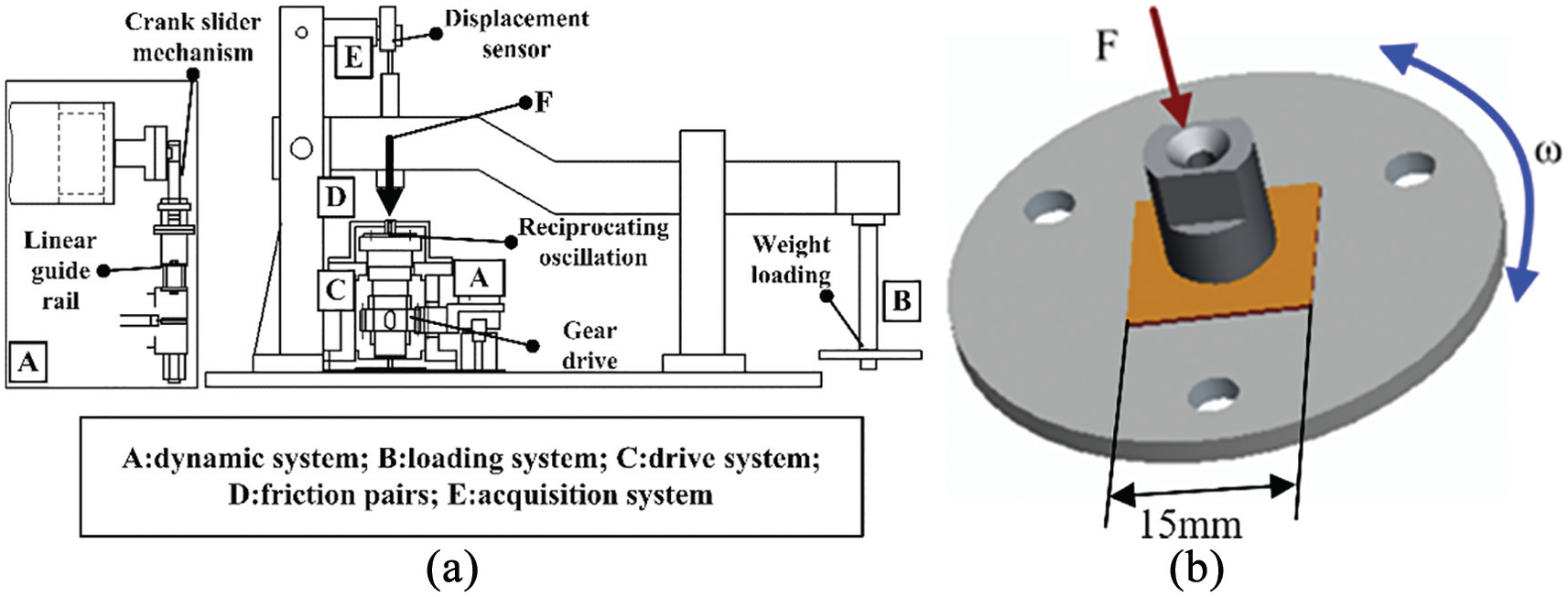
Heavy-load self-lubricating liner tester: (a) Schematic diagram of the tester and (b) Form of friction pair.

The GCr15 upper test piece was machined into a cylindrical pin with φ10 × 30 mm and a hardness of 50 HRC. The self-lubricating liner on the lower test piece was cut into a 15 × 15 mm² square. The liner had an original thickness of 0.34 mm. After cutting, the liner was bonded to the circular plate of 45 steel with phenolic resin as the adhesive at 180°C and 0.3 MPa for 2 h. In total, 10 samples were prepared under the same bonding process and tested under the same conditions using the same tester. The most critical characteristic parameter of the self-lubricating liner, the wear depth, was evaluated as the degradation parameter. Considering that GCr15 has a high degree of hardness and excellent wear resistance and that the wear depth between the friction pairs is mainly on the liner, the measured wear depth was taken as the wear depth of the liner. According to SAE AS 81820, the maximum wear depth of a heavy-load self-lubricating liner after 25,000 swings should be ≤0.114 mm. After 25,000 swings, the wear depths of the 10 groups of samples were measured, and the changes over time are shown in Figure 2.

Figure 2.

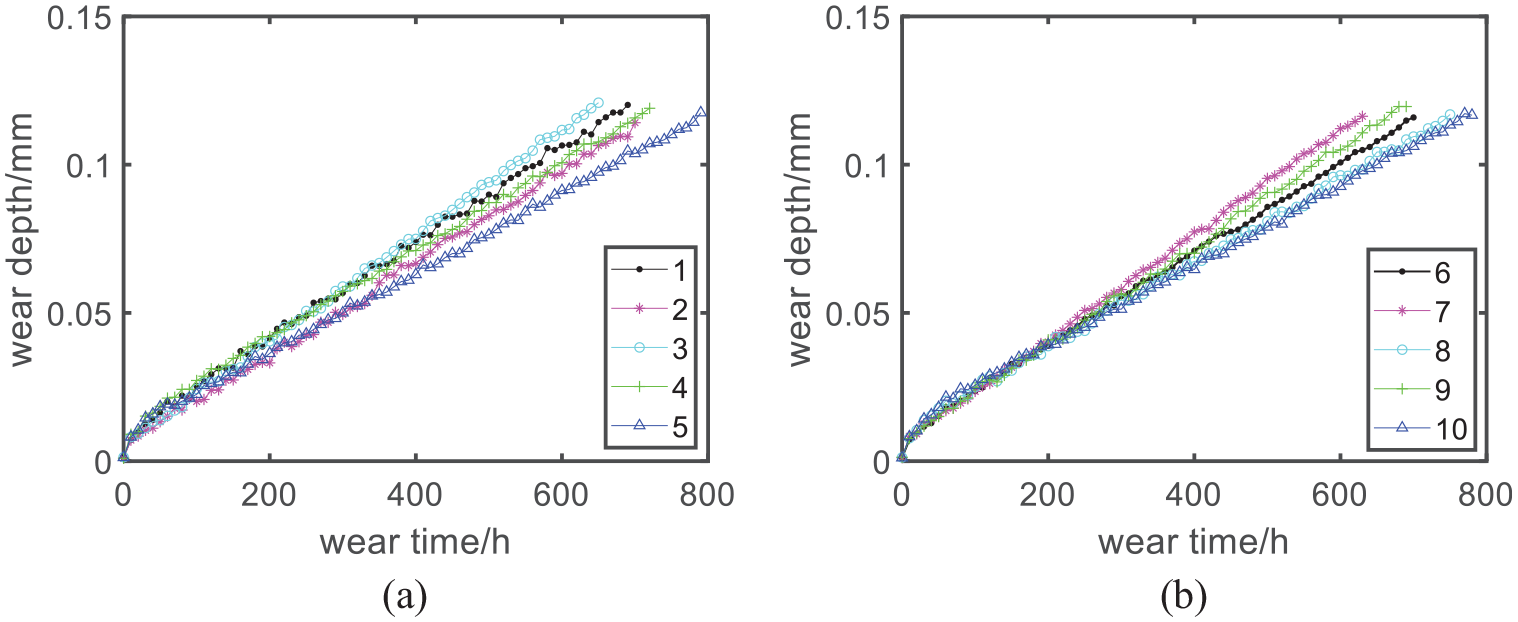
Wear depth curves of self-lubricating liners obtained from the life test: (a) wear depth of sample for 1–5 and (b) wear depth of sample for 6–10.

Data smoothing was performed to reduce the influence of various interferences and measurement errors. According to the failure concept based on first arrival times, the actual life values of the 10 samples obtained were 650, 700, 611, 691, 773, 687, 619, 740, 653, and 752 h. The lognormal, Weibull, and normal distributions were fitted to the 10 groups of life values to obtain the probability density function graphs, as shown in Figure 3.

Figure 3.

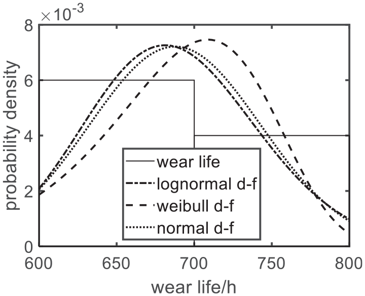
Distribution model of the wear life of the self-lubricating liner.

The Kolmogorov–Smirnov (K–S) test results of the wear life distribution fitting are shown in Table 1. h in the wear life K–S test results had the same value of 0, suggesting that the three distribution models were not rejected. In this case, the best distribution model was obtained according to the p-value. A comparison of the three models showed that the p-value of the lognormal distribution test result was the largest. Therefore, the wear life obeyed lognormal distribution.

Table 1.

K–S test of the wear life.

Test results	Lognormal d-f	Weibull d-f	Normal d-f
h	0	0	0
p	0.9886	0.9300	0.9518

The service life of the heavy-load self-lubricating liner obeyed the lognormal distribution. According to the characteristic parameters of the distribution function and reliability theory, the reliable life and average life of the self-lubricating liner at a reliability of 90% were found to be 618 and 688 h, respectively. The probability density function, reliability function, and failure rate function of the heavy-load self-lubricating liner can be obtained from the lognormal distribution parameters shown in Figure 4.

Figure 4.

Reliability index of the lognormal distribution parameters: (a) probability density function, (b) reliability function, and (c) failure rate function.

The probability density function in Figure 4 shows that the wear life values for this batch of heavy-load self-lubricating liners were mostly distributed around 700 h, and almost no liners had a life below 600 h. This indicates that this batch of heavy-load self-lubricating liners had relatively high stability. The failure rate function shows that when the wear time of the self-lubricating liners exceeded 620 h, the failure probability at the next moment increased rapidly; however, when the wear time was below 620 h, the failure rate of the self-lubricating liner was low. In addition, the reliability function shows that the heavy-load self-lubricating liner would not fail in the initial stage under the test conditions, suggesting that it could meet normal working requirements. However, when the wear time exceeded 600 h, the proportion of the self-lubricating liners that could continue to work normally declined. When the wear time exceeded 800 h, the proportion of self-lubricating liners that continued to work was almost zero. At a reliability of 90%, the heavy-load self-lubricating liner should be replaced with a new one when the wear time reaches 620 h.

Life prediction of self-lubricating kinematic pairs under heavy-load swinging conditions

The flow chart of the short-time and small-sample life prediction method based on Monte Carlo simulation is shown in Figure 5. The core objective of this method is to expand sample size using Monte Carlo simulation and an inverse transform method by taking the characteristic parameters as random events when the distribution model of the characteristic parameters is already known. As sample expansion is based on the characteristic parameter distribution model of the test samples, the prediction accuracy demonstrated relatively good adaptability and was not affected by the consistency of the product quality but was affected by sample size.

Figure 5.

Flowchart of the life prediction method with short-time and small-sample size.

To verify the validity of the short-time and small-sample life prediction method, an experimental scheme was formulated based on the uniform design method, where three samples were randomly selected from 10 test groups. In the following subsections, the samples from groups 1, 5, and 7 are used as examples to perform degradation trajectory fitting, establish a service life distribution model after expanding sample size, obtain reliability indices, and calculate prediction errors.

Degenerate trajectory fitting based on the support vector regression algorithm

According to the characteristics of the short-time and small-sample, as well as the liner wear process, wear depth data of the self-lubricating liner during the fast wear period were not considered. Only data between 30 h and 200 h in the full-life test were subjected to short-time life prediction. Sample wear depth curve fitting is the basis for accurately obtaining characteristic parameter data. Compared with the least square method, the support vector regression algorithm exhibits better fitting performance and is less affected by the dispersion of test data. The increasing trend of wear depth of the heavy-load self-lubricating liner during the stable wear stage was close to a straight line. Therefore, the linear support vector regression algorithm was used to fit the wear data in this study.

A linear model was established for each group of test data:

$$f\left(t\right)=\omega t+b$$

(1)

where f(t) is the predicted life; t is the prediction time point; ω represents the first characteristic parameter, the slope and wear rate; and b represents the second characteristic parameter, the intercept.

An appropriate parameter ε (ε > 0) was selected to construct an ε-band containing all the data points $(t_i,y_i)$ by translating the line (equation (1)) up and down along the y-axis by ε. Simultaneously, because of the discreteness of wear depth test data, the constraints could not be satisfied in most cases. Therefore, the relaxation variables ${\xi }_i$ and ${\xi }_i^{*}$ were introduced to allow the existence of points beyond the ε-band, and a penalty coefficient C was introduced for these points. The optimization problem was constructed as follows:

$$\begin{array}{c}min\frac{1}{2}\Vert \omega {\Vert }^2+C\sum _{i=1}^n({\xi }_i+{\xi }_i^{*})\hfill \\ \mathrm{s}.\mathrm{t}.y_i-\omega ·t_i-b_i\le \epsilon +{\xi }_i\hfill \\ \omega ·t_i+b_i-y_i\le \epsilon +{\xi }_i^{*}\hfill \\ {\xi }_i\ge 0\hfill \\ {\xi }_i^{*}\ge 0\hfill \\ i=1,2,\cdots ,n\hfill \end{array}$$

(2)

The above optimization problem (2) was solved using the Lagrange multiplier method. The calculation equation (3) for ω and the dual problem (4) of the optimization problem was performed.

$$\omega =\sum _{i=1}^n({\alpha }_i-{\alpha }_i^{*})t_i$$

(3)

$$\begin{array}{c}min\frac{1}{2}\sum _{i,j=1}^n({\alpha }_i-{\alpha }_i^{*})({\alpha }_j-{\alpha }_j^{*})(t_i·t_j)\hfill \\ +\epsilon \sum _{i=1}^n({\alpha }_i+{\alpha }_i^{*})-\sum _{i=1}^n{y}_i({\alpha }_i-{\alpha }_i^{*})\hfill \\ \mathrm{s}.\mathrm{t}.\sum _{i=1}^n({\alpha }_i-{\alpha }_i^{*})\hfill \\ 0\le {\alpha }_i\le C\hfill \\ 0\le {\alpha }_i^{*}\le C\hfill \\ i=1,2,\cdots ,n\hfill \end{array}$$

(4)

where ${\alpha }_i$ and ${\alpha }_i^{*}\ge 0$ are the Lagrange multipliers.

The solutions ${\alpha }_i$ and ${\alpha }_i^{*}$ can be obtained by solving the following convex quadratic programming problem.

$$\begin{array}{c}\overline{\alpha }={({\overline{\alpha }}_1,{\overline{\alpha }}_2,\cdots ,{\overline{\alpha }}_n)}^{\mathrm{T}}\hfill \\ {\overline{\alpha }}^{*}={({{\overline{\alpha }}^{*}}_1,{{\overline{\alpha }}^{*}}_2,\cdots ,{{\overline{\alpha }}^{*}}_n)}^{\mathrm{T}}\hfill \end{array}$$

(5)

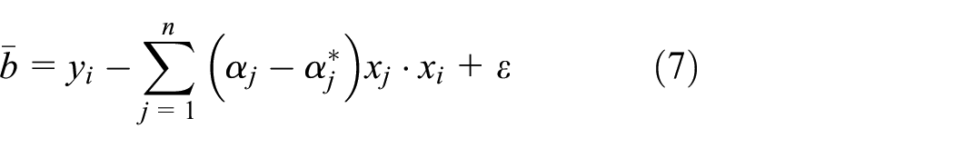
According to the Karush–Kuhn–Tucker condition, the necessary and sufficient conditions for solving convex programming, at the optimal point, which is the product of the Lagrange multiplier and the inequality constraint of the original problem, is equal to zero. Thus, the value of the second characteristic parameter can be calculated as follows:

When $0<{\alpha }_i<C$ ,

$$\overline{b}=y_i-\sum _{j=1}^n({\alpha }_j-{\alpha }_j^{*})x_j·x_i-\epsilon$$

(6)

Similarly, when $0<{\alpha }_i^{*}<C$ ,

$$\overline{b}=y_i-\sum _{j=1}^n({\alpha }_j-{\alpha }_j^{*})x_j·x_i+\epsilon$$

(7)

The following regression estimation function can be obtained:

$$f\left(t\right)=\sum _{i=1}^n({\alpha }_i-{\alpha }_i^{*})t_i·t+\overline{b}$$

(8)

By fitting the sample’s wear depth degradation trajectory, the characteristic parameter vectors of the wear rate and intercept can be obtained as follows:

$$\mathit{k}=\left[\begin{array}{ccc}1.5242\hfill & 1.3144\hfill & 1.6819\hfill \end{array}\right]\times {10}^{-4}$$

$$\mathit{b}=\left[\begin{array}{ccc}0.0079\hfill & 0.0100\hfill & 0.0068\hfill \end{array}\right]$$

Sample size expansion

Determination of the characteristic parameter distribution models

The lognormal, Weibull, and normal distributions were fitted to the first characteristic parameter vector to obtain the probability density function graphs, as shown in Figure 6. The expectation value and standard deviation for the fitted lognormal distribution were μ = −8.81 and σ = 0.12, respectively; the scale parameter and shape parameter for the fitted Weibull distribution were η = 1.57 × 10⁻⁴ and m = 11.20, respectively; and the expectation value and standard deviation for the fitted normal distribution were μ = −1.51 × 10⁻⁴ and σ = 1.84 × 10⁻⁵, respectively.

Figure 6.

Distribution model of the first characteristic parameter.

The K–S test results of the first characteristic parameter distribution fitting are listed in Table 2. The values of h in all K–S test results were 0, suggesting that the three distribution models were not rejected. In this case, the best distribution model was obtained according to the calculated p-values. A comparison of the three distribution models showed that the p-value of the normal distribution test result was the largest. Therefore, the first characteristic parameter obeyed normal distribution.

Table 2.

K–S test results of the first characteristic parameter fitting.

Test results	Lognormal d-f	Weibull d-f	Normal d-f
h	0	0	0
p	0.9293	0.9222	0.9500

Similarly, the probability density functions of the second characteristic parameter vector were obtained, as shown in Figure 7. The expectation value and standard deviation for the fitted lognormal distribution were μ = −4.81 and σ = 0.20, respectively; the scale parameter and shape parameter for the fitted Weibull distribution were η = 8.80 × 10⁻³ and m = 6.78, respectively; and the expectation value and standard deviation for the fitted normal distribution were μ = 8.20 × 10⁻³ and σ = 1.60 × 10⁻³, respectively.

Figure 7.

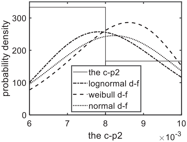
Distribution model of the second characteristic parameter.

According to the K–S test results given in Table 3, the second characteristic parameter obeyed lognormal distribution.

Table 3.

K–S test results of the second characteristic parameter.

Test results	Lognormal d-f	Weibull d-f	Normal d-f
h	0	0	0
p	0.9220	0.8383	0.8917

Sample size expansion

The first characteristic parameter obeyed normal distribution F, the range of which was [0,1]. First, the inverse function F⁻¹ of F was obtained through inverse transformation. Next, N uniformly distributed random numbers between 0 and 1 were generated by Monte Carlo simulation. Subsequently, the random numbers were substituted into F⁻¹ to obtain N random variables obeying normal distribution, that is, the expanded first characteristic parameters. The second characteristic parameters were also expanded using the same approach such that N random variables obeying the lognormal distribution (i.e. expanded second characteristic parameters) were obtained.

After expanding the characteristic parameters, N groups of life values (i.e. expanded sample) could be obtained by combining the degradation model and failure threshold for the heavy-load self-lubricating liner, as shown in Figure 8.

Figure 8.

Wear depth curves after sample expansion.

Service life prediction and reliability indices

The lognormal, Weibull, and normal distributions were fitted to the expanded life data for the heavy-load self-lubricating liner, as shown in Figure 9. The expectation value and standard deviation for the fitted lognormal distribution were μ = −6.56 and σ = 0.13, respectively. The scale parameter and shape parameter for the fitted Weibull distribution were η = 751.19 and m = 7.12, respectively. The expectation value and standard deviation for the fitted normal distribution were μ = 708.82 and σ = 112.72, respectively.

Figure 9.

Distribution model of the expanded life of the self-lubricating liner.

According to the K–S test results given in Table 4, the life of the heavy-load self-lubricating liner obeyed lognormal distribution.

Table 4.

K–S test results of the expanded life.

Test results	Lognormal d-f	Weibull d-f	Normal d-f
h	0	0	0
p	0.8590	0.4123	0.6143

The service life of the heavy-load self-lubricating liner obeyed lognormal distribution. According to the characteristic parameters of its distribution function and reliability theory, we can conclude that at a reliability of 90%, the reliable life of the self-lubricating liner was 596 h, the average life was 709 h, and the error was 3.05%.

Influence of test samples on life prediction accuracy

To verify the validity of the short-time small-sample life prediction method, an experimental scheme was formulated based on a uniform design method, where three samples were randomly selected from the 10 test groups. The selected samples were then used to perform degradation trajectory fitting, establish a service life distribution model after expanding the sample size, obtain reliability indices, and calculate the prediction errors, as shown in Table 5.

Table 5.

Prediction errors of different sample life values.

Verification scheme	Sample number	Reliable life (h)	Average life (h)	Error (%)
1	1, 5, 7	596	709	3.05
2	2, 10, 3	557	665	3.34
3	3, 4, 10	567	671	2.47
4	4, 9, 6	633	653	5.09
5	5, 3, 2	581	724	5.23
6	6, 8, 9	606	673	2.18
7	7, 2, 5	609	722	4.94
8	8, 7, 1	583	665	3.34
9	9, 1, 8	606	669	2.76
10	10, 6, 4	611	663	3.63

As seen in Table 5, the predicted average lives for different sample combinations were different, and the difference between the highest and lowest predicted average life value was 71 h. The predicted reliable life for different sample combinations was also different, and the difference between the highest and lowest predicted reliable life value was 76 h. The life prediction errors obtained from the three samples were all relatively small; the maximum error was 5.23%.

The basis for sample expansion is the distribution model of its fundamental characteristic parameters. But the sample number directly affects the accuracy of the prediction. Table 6 shows that the number of samples increased one-by-one based on scheme 7 given above. After the sample size was expanded, the life prediction error decreased.

Table 6.

Prediction errors of different sample sizes.

Verification scheme	Added sample number	Reliable life (h)	Average life (h)	Error (%)
1	-	609	722	4.94
2	1	593	716	4.07
3	1,3	578	675	1.89
4	1, 3, 4	575	673	2.18
5	1, 3, 4, 6	593	678	1.45

For the characteristic distribution model obtained from the same sample size, if the expanded sample sizes were different, the life prediction results varied to a certain extent because of the randomness of sample expansion. To analyze the influence of the expanded sample size on the prediction results, groups 1, 5, and 7 were used as examples to perform sample expansion. The sample size was expanded to 50, 100, 200, and 300, respectively, and the expansion was performed three times for each expanded sample size, as shown in Table 7.

Table 7.

Prediction error with different expanding sample size.

Expanded sample size	Expansion times	Reliable life (h)	Average life (h)	Error (%)
50	1	513	657	4.51
	2	588	718	4.36
	3	529	670	2.62
100	1	596	709	3.05
	2	567	671	2.47
	3	585	704	2.33
200	1	578	705	2.47
	2	554	670	2.62
	3	606	708	2.91
300	1	581	705	2.47
	2	553	669	2.76
	3	551	672	2.33

The expansion results in Table 7 show that the life prediction results also exhibited certain randomness for the same expanded sample size. In general, a larger expanded sample size resulted in a smaller prediction error. However, there could be cases where both sample size and prediction errors were large.

In summary, the sample size should reach a certain number when the sample is being expanded. This number is related to the consistency of product quality. Inconsistent product quality requires more samples to be expanded to eliminate the errors caused by the randomness of sample expansion.

The prediction values of the reliability indices between different sample combinations differed due to the consistency of the life test. The difference in the wear rate for each group of tests led to different prediction results. The life test consistency for the heavy-load self-lubricating liner was affected by test sample preparation, test operation, tester status, and environmental factors. The consistency of sample preparation was affected by the amount and uniformity of glue applied during the preparation process, the surface roughness, and other factors.

In order to study the effect of the quality consistency on life prediction accuracy, the test pressure was raised to P = 200 MPa and f = 0.4 Hz. All tests were performed at room temperature (15°C–25°C) and under a relative humidity of 35 ± 8%. The wear depths of the 10 groups of samples were measured, and are shown in Figure 10.

Figure 10.

Wear depth curves of self-lubricating liners obtained from the life test: (a) wear depth of sample for 1–5; (b) wear depth of sample for 6–10.

After data smoothing and based on the first arrival times, the actual life values of the 10 samples obtained were 155, 163.5, 97.5, 112.5, 131, 107, 144.5, 92, 131.5, and 158 h. The life of the self-lubricating liners obviously decreased and the wear rates increased with the test pressure and swing frequency increasing. Based on a uniform design method, three samples were randomly selected, and the degradation trajectory of the wears were fitted. The service life distribution model and the average life after expanding the sample size were obtained. The prediction errors are shown in Table 8.

Table 8.

Prediction errors of different sample life values.

Verification scheme	Sample number	Reliable life (h)	Average life (h)	Error (%)
1	1, 5, 7	115	145	12.19
2	2, 10, 3	89	146	12.96
3	3, 4, 10	84	122	5.61
4	4, 9, 6	98	117	9.48
5	5, 3, 2	82	136	5.22
6	6, 8, 9	84	112	13.35
7	7, 2, 5	81	137	6.00
8	8, 7, 1	84	132	2.13
9	9, 1, 8	83	126	2.51
10	10, 6, 4	98	125	3.29

When the dataset sizes were relatively small, namely 3, the life prediction accuracy was decreased because of the poor consistency of the wear rate. Now, the number of samples should be increased. Based on scheme 1 and with the number of samples increasing step by step, the prediction errors with the short-time small-sample life prediction method can be shown in Table 9. Table 9 indicates that the accuracy of life prediction increases with the sample size increasing. So, the number of samples should be as large as possible when the consistency of sample quality is poor.

Table 9.

Prediction errors of different sample sizes.

Verification scheme	Added sample number	Reliable life (h)	Average life (h)	Error (%)
1	–	115	145	12.19
2	2	120	147	13.73
3	2, 3	97	138	6.77
4	2, 3, 4	96	134	3.68
5	2, 3, 4, 6	94	132	2.13

Conclusion

During the stable wear stage of heavy-load self-lubricating liners, the wear depth was observed to increase linearly. The first characteristic parameter (i.e. wear rate) obeyed normal distribution, and the second characteristic parameter (i.e. intercept) obeyed lognormal distribution. After expanding the sample size by Monte Carlo simulation, the service lives of the batch of samples could be obtained according to the failure criterion, which was found to agree with logarithmic normal distribution. After expanding any three selected samples to a sufficient sample size, the calculated error of service life prediction could meet the requirements for evaluating the lifecycle during product R&D. This provides a theoretical basis for shortening the R&D cycle of heavy-load self-lubricating liners and self-lubricating spherical plain bearing products and can also serve as a reference for predicting the lives of other mechanical parts with gradual degradation.

Although the short-time small-sample life prediction method based on Monte Carlo simulation exhibited a relatively high prediction accuracy, it required a high-precision curve fitting of the degradation curve of the test sample. Simultaneously, its accuracy was also affected by factors such as sample size expansion and randomness, the quality of the test sample, the degradation measurement accuracy, and the status of the tester. This method is applicable for the life prediction of mechanical parts and electronic components with linear or non-linear degenerate variable, but a degradation trajectory function must be clarified. If a degradation law is not available, the method cannot be applied.