Sage Journals: Discover world-class research

Abstract

Rolling bearings are the key components of rotating machinery. Incipient fault diagnosis of bearing plays an increasingly important role in guaranteeing normal and safe operation of rotating machinery. However, because of the high complexity of the fault feature extraction, the incipient faults of rolling bearings are difficult to diagnose. To solve this problem, this paper presents a new incipient fault intelligent identification method of rolling bearings based on variational mode decomposition (VMD), principal component analysis (PCA), and support vector machines (SVM). In the proposed method, the bearing vibration signals are decomposed by using VMD, and a series of intrinsic mode functions (IMFs) with different frequencies are obtained. Then, the energy and kurtosis values of each IMF are calculated to reveal the intrinsic characteristics of the vibration signals in different scales. Finally, all energy and kurtosis values of IMFs are processed via PCA and subsequently fed into SVM to achieve the bearing fault identification automatically. The effectiveness of this method is verified through the experimental bearing data. The verification results indicate that the proposed method can effectively extract the bearing fault features and accurately identify the bearing incipient faults, and outperform the two compared methods obviously in identification accuracy and computation time.

Keywords

Incipient rolling bearing faults intelligent identification energy and kurtosis variational mode decomposition principal component analysis support vector machine

Introduction

Rolling bearings are widely used in all kinds of rotating machinery equipment because of their good performance and easy manufacture.¹ As the key components connecting rotating parts and fixed parts of rotating machinery, rolling bearings will greatly affect the overall performance and safe operation state of rotating machinery.² Therefore, it is very necessary to identify the rotating machinery faults, especially the incipient faults of rolling bearings. Unfortunately, due to the heavy nonlinear dynamic behavior of the rotor-bearing system, complex and harsh operation environment, and some random interference, the sampled vibration signals of rolling bearing faults usually exhibit the obvious non-stationary characteristics.³ In this situation, weak fault vibration signals are difficult to be effectively analyzed by traditional signal processing methods, which may result in low accuracy of incipient fault identification of rolling bearings.

In order to identify the incipient faults of rolling bearings accurately and efficiently, all kinds of advanced signal processing techniques are employed to analyze the vibration signals of rolling bearings.^4–8 The novel time-frequency analysis methods such as empirical mode decomposition (EMD),⁹ empirical wavelet transform (EWT),¹⁰ and variational mode decomposition (VMD)¹¹ are powerful and effective tools for processing non-stationary signals, and these methods have been widely used for vibration signal processing, condition monitoring, and fault identification of rolling bearings in the past several years.^12,13 However, EMD has inherent modal aliasing phenomenon and endpoint effect,⁹ and also it is difficult to explicitly construct the frequency bands of EWT.¹¹ In this situation, EMD or EWT-based fault diagnosis methods cannot achieve the effective signal analysis and accurate fault identification of rolling bearings. Over the recent years, deep learning-based intelligent fault diagnosis methods of rolling bearings have been widely and successfully developed, because they can learn discriminant fault features from raw data by deep structure with multi-layers of non-linear data processing units.¹⁴ However, the architectures of deep learning networks are often determined by trial and modification, so these neural networks are lack of interpretability for fault diagnosis tasks. Besides, the traditional deep learning approaches have low diagnosis accuracy and slow convergence speed.¹⁵ Especially, the excellent performance of deep learning models needs a large number of data samples to support, and it is undoubted that the traditional deep learning approaches couldn’t work well for accurate fault pattern recognition once the number of data samples is limited.

As an advanced signal processing approach, VMD, proposed by Dragomiretskiy and Zosso,¹¹ has outstanding performance on processing non-stationary and nonlinear signals, which can adaptively decompose a complex signal into its relative simple principal modes with different frequencies to realize the effective separation of each component. In the process of signal decomposition, the VMD algorithm searches the optimal solution of the variational model by iterative computation to determine the frequency center and bandwidth of each component so that it can obtain more accurate intrinsic mode functions (IMFs) of the signal. Thus, compared with the other two methods mentioned above, it is obvious that VMD has more powerful ability in conducting non-stationary mechanical vibration signals, and this method has attracted more and more attention in the field of fault diagnosis.^16–24 Ma et al.¹⁸ studied the incipient fault feature extraction method of rolling bearings based on the modified VMD and Teager energy operator (TEO) to accomplish the accurate identification of fault types, and by comparing with local mean decomposition (LMD), it is found that VMD can extract fault feature information more effectively. A novel method for rolling bearing fault diagnosis based on variational mode decomposition was presented by Zhang et al.,¹⁹ and a comparison research of bearing fault signals is done between VMD and EMD, the result of which verifies the VMD can accurately extract the principal mode of bearing fault signal and is better than EMD in bearing defect characteristic extraction. He et al.²⁰ presented an integrated method for weak fault detection of rolling bearings based on minimum entropy deconvolution and VMD, and demonstrated that the method is more robust than spectral kurtosis and EWT in extracting the weak fault characteristics. Moreover, some literatures^21–24 also report that the VMD or improved VMD algorithm can more effectively extract fault feature information from the vibration signals of rolling bearings.

Fault types of rolling bearings can be automatically identified by using some machine learning methods when the useful fault features (quantitative characteristics of different fault statuses) have been successfully extracted.^3,17,25–27 PCA can compress the dimension of sample feature space, simplify the complexity of computation process, and improve the efficiency and accuracy of object classification.²⁸ Meanwhile, SVM model has the outstanding advantages in learning the intrinsic knowledge of the small sample, nonlinear, and high-dimensional data.²⁹ And consequently, as an important data processing and classification technique, the integrated approach based on principal component analysis combined with support vector machine (PCA-SVM) has been widely applied to all kinds of pattern recognition problems,³⁰ especially to fault status identification.³¹ For the complex industrial process, related scholars researched the feature extraction and fault classification methods of Tennessee Eastman Process (TEP) based on PCA and SVM.^32,33 The different status of TEP can be effectively detected and predicted via the perspective diagnosis method. Normal and safe operation of the any electrical equipment and power system is the key to the power grid, so the common faults of the transformers and power system were analyzed and accurately diagnosed by using the hybrid PCA-SVM techniques.³⁴ In order to maintain efficient and safe operation of the rotating machinery, several fault diagnosis approaches based on PCA and SVM were presented and used to recognize the different fault status of rolling bearings and rotors.³⁵ These methods can achieve accurate fault detection and identification, so PCA and SVM actually have the excellent performance in fault feature extraction and fault classification.

Based on the above analysis, here we present a vibration signal processing and classification method for incipient fault identification of rolling bearings based on VMD and PCA-SVM schemes. In our proposed method, the sampled vibration signals are decomposed into a series of components and the quantitative features (energy and kurtosis) of each component are computed to characterize the different incipient fault status of rolling bearings. After that, PCA algorithm is implemented on the obtained quantitative features, so more concise and more effective fault features can be largely extracted. In the last stage, the feature data is conducted by using SVM classifier. Subsequently, the verification experiments are implemented on two bearing fault data sets and the results indicate that the proposed method really has a better performance than some of the current state of the art in rolling bearing fault diagnosis. Under the condition of small samples, the method actually achieves a more accurate fault recognition rate and a faster computation speed than other two important methods which are the EMD-based method and the deep learning approach.

The rest of this paper is organized as follows. Section 2 introduces the related basic theories, including signal decomposition algorithm (VMD), quantitative signal features (energy and kurtosis), and feature extraction combined with data classification method (PCA-SVM). In Section 3, we detail the proposed incipient fault identification method including vibration signal decomposition, fault feature extraction, and fault pattern recognition. Meanwhile, the key parameters of VMD, PCA, and SVM are discussed. Section 4 verifies the performance of the proposed method via experiment fault data. And finally, the conclusions are drawn in Section 5.

Related basic theories

Variational mode decomposition

Variational mode decomposition, drastically developed and widely used in recent years, is a fully intrinsic and adaptive signal decomposition method and suitable for processing nonstationary signals. It has the strict mathematical theories including classical Wiener filtering, Hilbert transform, and heterodyne demodulation, and this method can adaptively decompose a complex multi-component input signal x(t) into several intrinsic mode functions u_k(t) (k = 1, …, K) with the finite bandwidth.¹¹ On the other hand, the original signal can be accurately reconstructed by generally summing all the mode functions. The essence of VMD is to construct a constrained variational model and find its optimal solution to obtain a separate number of mode components and their corresponding center frequencies under the condition of minimizing the sum of all the mode bandwidth estimation. In the process of signal decomposition, each mode function component u_k(t) which has the specific sparsity and the finite bandwidth is automatically computed according to the corresponding center frequency.²¹ And the complete VMD algorithm can be succinctly described as follows.

In order to obtain the estimation of mode bandwidth, each mode function u_k(t) is conducted by Hilbert transform, and then its analytic signal is expressed as:

[δ (t) + \frac{j}{π t}] * u_{k} (t)

(1)

Subsequently, the center frequency of each mode estimation is modulated to the base band by using the exponential factor e^−jω_kt, written as:

[(δ (t) + \frac{j}{π t}) * u_{k} (t)] e^{- j ω_{k} t}

(2)

Furthermore, the L₂ norm of the gradient of the analytic signal in equation (2) is calculated, and the bandwidth of each mode function is also estimated. Consequently, the mode estimation becomes a bandwidth-constrained variational problem which is employed by the VMD algorithm to obtain the intrinsic mode functions, and its mathematical model can be expressed as:

{\begin{matrix} min_{{u_{k}}, {ω_{k}}} {\sum_{k = 1}^{K} {‖ \partial_{t} [(δ (t) + \frac{j}{π t}) * u_{k} (t)] e^{- j ω_{k} t} ‖}_{2}^{2}} \\ s . t . \sum_{k = 1}^{K} u_{k} (t) = x (t) \end{matrix}

(3)

where {u_k} and{ω_k} are the shorthand notations of the set of all modes and their center frequencies, respectively, ∂_t is the partial derivative operator and * denotes convolution.

In order to find the optimal solution of equation (3), Lagrangian multipliers λ(t) and a penalty term α are conjointly utilized to render the above problem unconstrained. The combination of these two terms guarantees the strict constraint condition and the nice convergence properties. Therefore, the augmented Lagrangian function L can be constructed as follows:

\begin{matrix} L ({u_{k}}, {ω_{k}}, λ) = α \sum_{k = 1}^{K} {‖ \partial_{t} [(δ (t) + \frac{j}{π t}) * u_{k} (t)] e^{- j ω_{k} t} ‖}_{2}^{2} \\ + ‖ x (t) - \sum_{k = 1}^{K} u_{k} (t) ‖_{2}^{2} \\ + 〈 λ (t), x (t) - \sum_{k = 1}^{K} u_{k} (t) 〉 \end{matrix}

(4)

The optimal solution of equation (3) is now to search the saddle point of the augmented Lagrangian function L. The saddle point can be easily found by using alternate direction method of multipliers, so the intrinsic mode is expressed as:

{\hat{u}}_{k}^{n + 1} (ω) = \frac{\hat{x} (ω) - \sum_{i \neq k} {\hat{u}}_{i} (ω) + \frac{\hat{λ} (ω)}{2}}{1 + 2 α (ω - ω_{k})}

(5)

which is equally treated as a Wiener filtering of the mode component, and the mode in time domain can be obtained by implementing inverse Fourier transform of this filtered signal. And meanwhile, the corresponding center frequency is given as:

ω_{k}^{n + 1} = \frac{\int_{0}^{\infty} ω {| {\hat{u}}_{k} (ω) |}^{2} d ω}{\int_{0}^{\infty} {| {\hat{u}}_{k} (ω) |}^{2} d ω}

(6)

which aims to set the new ω_k at the center of the power spectrum of the corresponding mode.

On the basis of the theory mentioned above, the key steps of the complete algorithm for VMD are summarized in Algorithm 1.

Algorithm 1. Complete optimization process of VMD
Input: A real valued signal x Output: A number of sub-signals (modes) ${{\hat{u}}_{k}}$ Initialize ${{\hat{u}}_{k}^{1}}$ , ${ω_{k}^{1}}$ , ${\hat{λ}}^{1}$ , $n = 0$ repeat $n = n + 1$ fork = 1: K do Update ${\hat{u}}_{k}$ and $ω_{k}$ according to equations (5) and (6) end for Update $\hat{λ}$ according to the following equation ${\hat{λ}}^{n + 1} (ω) = {\hat{λ}}^{n} (ω) + τ (\hat{x} (ω) - \sum_{k = 1}^{K} {\hat{u}}_{k}^{n + 1} (ω)) (7)$ until satisfy the convergence condition: $\sum_{k = 1}^{K} \frac{‖ {\hat{u}}_{k}^{n + 1} - {\hat{u}}_{k}^{n} ‖_{2}^{2}}{‖ {\hat{u}}_{k}^{n} ‖_{2}^{2}} < ε (8)$ Implement inverse Fourier transform on ${{\hat{u}}_{k} (ω)}$ return ${{\hat{u}}_{k}}$

Algorithm 1. Complete optimization process of VMD

Input: A real valued signal x
Output: A number of sub-signals (modes)

{{\hat{u}}_{k}}

Initialize

{{\hat{u}}_{k}^{1}}

{ω_{k}^{1}}

{\hat{λ}}^{1}

n = 0

repeat

n = n + 1

fork = 1: K do
Update

{\hat{u}}_{k}

and

ω_{k}

according to equations (5) and (6)
end for
Update

\hat{λ}

according to the following equation

{\hat{λ}}^{n + 1} (ω) = {\hat{λ}}^{n} (ω) + τ (\hat{x} (ω) - \sum_{k = 1}^{K} {\hat{u}}_{k}^{n + 1} (ω)) (7)

until satisfy the convergence condition:

\sum_{k = 1}^{K} \frac{‖ {\hat{u}}_{k}^{n + 1} - {\hat{u}}_{k}^{n} ‖_{2}^{2}}{‖ {\hat{u}}_{k}^{n} ‖_{2}^{2}} < ε (8)

Implement inverse Fourier transform on

{{\hat{u}}_{k} (ω)}

return

{{\hat{u}}_{k}}

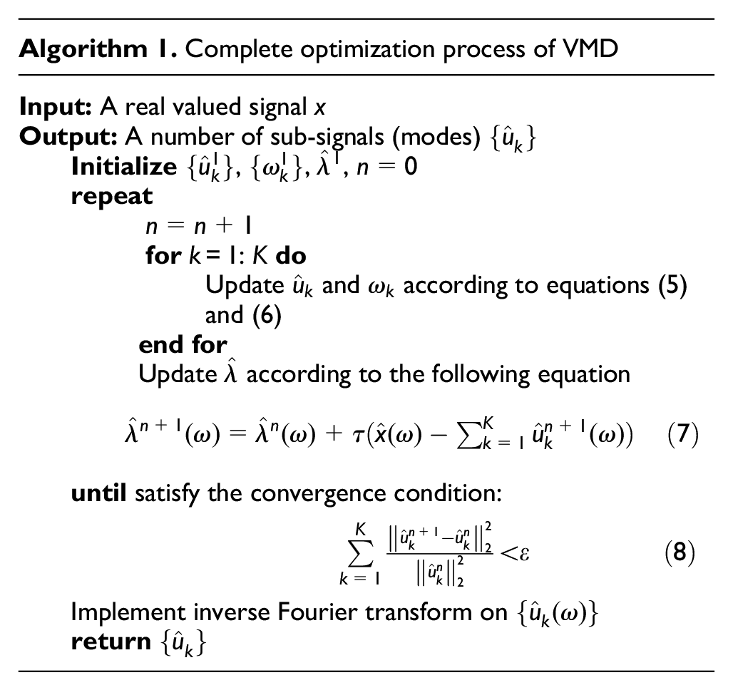
For each iteration in Algorithm 1, all the intrinsic modes are computed on the basis of the previous results and orderly updated, and equation (8) can effectively constrain the small error of each mode.

Signal energy and kurtosis

There are lots of statistical measures which can be used for representing the characteristics of a signal, including mean, variance, energy, covariance, skewness, kurtosis, and so on. For the vibration signal of rolling bearings, energy and kurtosis are the two ones of the most sensitive and effective statistics. Estimation of signal energy is a commonly used measurement in engineering analysis, and it can accurately reflect the intensity of the vibration signal acquired from operating rolling bearings.³⁶ Kurtosis is a classical measure which is used to describe the peakedness of the distribution of observed data points near the mean, and it is much more sensitive to the spikes in the data. Therefore, it is particularly suitable for detecting the periodic pulse components in the vibration signal of rolling bearings.³⁷ So, the two statistics are widely used to quantify the vibration behavior of rolling bearings.

Traditionally in signal processing, for a continuous-time real valued signal x(t), the energy En of the signal is defined using the integral of squared signal magnitude in a finite time interval, that is,

En = \int_{0}^{T_{0}} {| x (t) |}^{2} d t

(9)

and correspondingly, for a discrete-time real valued signal x(n), the energy En of the signal is defined using the sampling frequency average of the sum of the squared signal magnitude at each sampling point, that is,

En = \frac{1}{f_{s}} \sum_{n = 1}^{N} {| x (n) |}^{2}

(10)

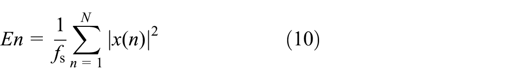
where f_s is the sampling frequency.

Generally in data analysis, for a random variable x, the kurtosis Ku of the random variable x is defined as:

Ku = \frac{E {(x - μ)}^{4}}{σ^{4}}

(11)

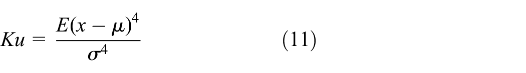
where μ is the mean of x, σ is the standard deviation of x, and E(t) represents the mathematical expectation of the quantity t.

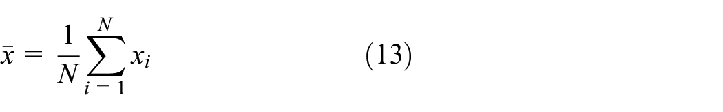
In engineering practice, the random variable x is usually unknown, but we can acquire a group of samples x = {x₁, x₂, …, x_N} of x. And the kurtosis of sample set x can be expressed as:

Ku = \frac{N \sum_{i = 1}^{N} {(x_{i} - \bar{x})}^{4}}{{(\sum_{i = 1}^{N} {(x_{i} - \bar{x})}^{2})}^{2}}

(12)

where $\bar{x}$ is the mean of sample set x, that is,

\bar{x} = \frac{1}{N} \sum_{i = 1}^{N} x_{i}

(13)

From the mathematical view, kurtosis is a dimensionless statistical metric for quantifying the non-Gaussianity of an arbitrary probability distribution. Therefore, kurtosis can represent the extent to which the vibration pattern of rolling bearings deviates from the normal operating status. Especially, when the incipient faults of rolling bearings occur, the kurtosis of bearing vibration signals drastically becomes large.

As shown in Figure 1, the energy and kurtosis values of two real valued signals within a limited time range are computed out, respectively. It can be clearly seen that the time domain waveforms, energy values and kurtosis values of the two signals are obviously different and the two signals have some their own characteristics. The upper signal contains lots of periodic impulses, while the lower signal consists of relatively stable, large, and continuously varying components. According to the statistics theory, the standard deviation of the lower signal sequence is certainly larger than that of the upper signal sequence, while the mean values of them are almost equal. That’s why the energy value of the lower signal is larger than that of the upper signal while the kurtosis value of the upper signal is larger than that of the lower signal. Therefore, the energy and kurtosis actually can characterize the distinctions of different signals effectively.

Figure 1.

Energy and kurtosis values of two different signals.

Principal component analysis and support vector machine

Principal component analysis is a multivariate statistical technique, and this linear transform has been widely applied in data analysis and compression. It analyzes the covariance structure of multivariate statistical observation data in order to find the principal components (PCs) which can simply express the dependence relationship between these data.³⁸ The basic principle of PCA for a two-dimensional variable data set can be illustrated in Figure 2.

Figure 2.

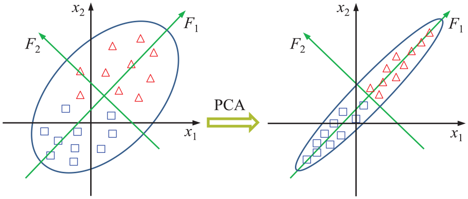
Illustration of PCA for a two-dimensional variable data set.

As shown in Figure 2, the essence of PCA is to transform the coordinate system of the original feature data variables through translation and rotation on condition that the information of the original variables can be maintained to the greatest extent, and the coordinate axes are transformed to the most prominent direction of the feature data variables’ variation and the vertical direction. In other words, the goal of translation and rotation is to make the data samples have maximum dispersion along F₁ axis, that is, the maximum variance along F₁ axis. Actually, if the original data can be represented by one feature F₁ instead of two features x₁ and x₂, it can be ensured that the new coordinate system can achieve dimension reduction under the principle of maintaining the important information of original variables as much as possible. The detailed implementation process of the PCA method is described as follows.

Given a sample set X = {x₁, x₂, …, x_N} $\subset$ Rⁿ in input space, let

μ = \frac{1}{N} \sum_{i = 1}^{N} x_{i}

(14)

and the covariance matrix of the sample set is defined as:

C = \frac{1}{N} \sum_{i = 1}^{N} (x_{i} - μ) {(x_{i} - μ)}^{T}

(15)

The core problem of PCA is to solve the characteristic equation of $C$

λ v = Cv

(16)

where $λ \geq 0$ is the eigenvalue, and $v \subset R^{n}$ is the eigenvector.

Assume that $λ_{i}, v_{i} (i = 1, 2, \dots, n)$ are the eigenvalues and corresponding eigenvectors of equation (16), respectively. The dimension compression of the original data set, on the premise of minimum mean square error, is to find a set of new features to replace the original features, and this set of features can maintain as much original feature information as possible. According to this principle, let λ₁ ≥ λ₂ ≥ … ≥λ_n, and the contribution rate of the ith principal component is defined as:

χ_{i} = \frac{λ_{i}}{\sum_{k = 1}^{n} λ_{k}}

(17)

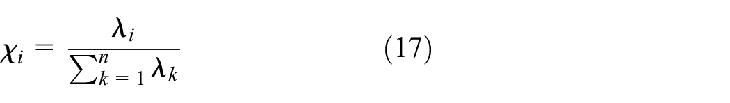
And the cumulative contribution rate of the first m principal components is expressed as:

ζ = \frac{\sum_{i = 1}^{m} λ_{i}}{\sum_{k = 1}^{n} λ_{k}} = \sum_{i = 1}^{m} χ_{i}

(18)

If $ζ$ reach the given value, the feature space formed by the first m eigenvectors can be regarded as the low-dimensional projection space after dimension reduction, that is,

Y = V^{T} (X - μ)

(19)

where V = [v₁, v₂, …, v_m], and the ith component of Y is the ith principal component of X. Thus, a few new variables are found to replace the original feature variables of X. From the perspective of data compression, the useful information of the input set is retained to the maximum extent while the feature dimension is reduced. The transformation from high-dimensional space to low-dimensional space is realized, and the complex problems become relatively simple and easy. So, PCA is actually a useful feature extraction method.

Support vector machine is a supervised machine learning method, and it is built on the basis of the structural risk minimization principle and Vapnik-Chervonenkis dimension theory of statistical learning theory.³⁹ SVM model is skilled in dealing with small sample and nonlinear data, and consequently SVM can achieve accurate nonlinear data classification and status prediction. Actually, it carries out binary classification by constructing a maximal margin hyperplane between the two classes of observed samples.

SVM is developed from the optimal classification hyperplane in the case of linearly classifiable situation. Its basic idea is to form a line or a hyperplane between two types of data sets to correctly separate them. This can be illustrated by the data with two dimensions shown in Figure 3.

Figure 3.

Diagram of optimal classification hyperplane for linearly classifiable data with two dimensions.

As shown in Figure 3, the square “□” and triangle “Δ” represent the samples of the two types of data respectively; H is the classification line, which separates the two types of data samples without error; H₁ and H₂ are the lines passing through the samples closest to the classification line and parallel to the classification line, and the distance between them is called the classification margin; the solid samples respectively passed by H₁ and H₂ are called support vectors (SVs).

In fact, there are an infinite number of classification lines H that can separate the two types of samples without error, and the classification line H^* with the maximum classification margin is called the optimal classification line, which not only correctly separates the two types of samples, but also maximizes the classification margin. When the two-dimensional space is extended to the high-dimensional space, the optimal classification line can be extended to the optimal classification hyperplane.

For linearly classifiable data sets, SVM model maximizes the margin or equivalently solves the corresponding convex quadratic programming problem to obtain the classification hyperplane

ω^{T} x + b = 0

(20)

where x is the support vector (sample data), ω is the weight vector, and b is the bias. Therefore, the corresponding decision function can be given by

f (x) = sign (ω^{T} x + b)

(21)

For linearly unclassifiable data sets, the general scheme is to introduce a slack variable ξ, so the linearly unclassifiable problem is transformed into the following optimization problem, that is,

{\begin{matrix} min J (ω, ξ) = \frac{{‖ ω ‖}^{2}}{2} + η \sum_{i = 1}^{N} ξ_{i} \\ s . t . {\begin{matrix} y_{i} (ω^{T} x + b) - 1 + ξ_{i} \geq 0 \\ ξ_{i} > 0, i = 1, 2, \dots, N \end{matrix} \end{matrix}

(22)

where η is the penalty parameter, y_i is the class label, and N is the number of input samples. For the binary classification problem, y_i is assigned −1 or +1. Then, the classification hyperplane and the decision function are obtained by solving equation (22). Using the kernel function, the decision function of the nonlinear SVM can be expressed as

f (x) = sign [\sum_{i = 1}^{N} α_{i} y_{i} K (x_{i}, x) + b]

(23)

where α_i are Lagrange multipliers, and K(·,·) is a kernel function. Commonly, used kernel functions are several possibilities. In this paper, Gaussian kernel is chosen, that is,

K (x_{i}, x_{k}) = \exp (- \frac{{‖ x_{i} - x_{k} ‖}^{2}}{2 h^{2}})

(24)

where h is the bandwidth, which affects the transformation of data. Therefore, the value of h is able to control the performance of SVM.

Proposed method

Bearing fault diagnosis is essentially a particular pattern recognition problem. Generally, fault diagnosis contains signal acquisition, feature extraction, and fault identification.⁴⁰ Fault feature extraction and identification play an important role in fault diagnosis, and they profoundly affect the accuracy of diagnosis results. In this section, we aim to develop an intelligent diagnosis method based on VMD and PCA-SVM techniques to achieve accurate incipient fault identification of rolling bearings. In the beginning of the method, VMD is applied to decompose the bearing fault vibration signal into a series of IMFs, and subsequently the energy and kurtosis of each IMF component are calculated to construct the original fault feature data. After that, we implement PCA on the original fault feature data to extract more concise and more effective fault features. In the fault identification, finally, SVM is employed to classify the extracted feature data corresponding to the different faults. The SVM classifier can effectively learn the knowledge of the incipient fault characteristics of rolling bearings from the extracted feature data. The overall process is shown in Figure 4.

Figure 4.

Overall process of the proposed method for incipient fault diagnosis of rolling bearings.

For the proposed method, some details need to be addressed here. Firstly, the two parameters K (the number of IMFs) and α (the penalty term) are of great importance to the VMD algorithm.¹¹ Actually, they principally determine the decomposition result of any signal. Therefore, the suitable parameters are largely useful for obtaining more accurate decomposition results. On the basis of the previous researches about the fault vibration signal decomposition of rolling bearings,^22–24 we set that the two parameters are equal to the common values (i.e. K = 5 and α = 2000). Secondly, for PCA, the useful PCs carry most of important characteristic information and play a key role in data classification. And consequently, the cumulative contribution rate of PCs which can determine the number of useful PCs is assigned as 85% according to some attractive findings in feature extraction and dimensionality reduction for rolling bearing fault detection and diagnosis.^41–43 Thirdly, the original SVM model is only able to achieve the binary classification, but multi-class classification is the most case in the practical fault diagnosis problem. So, an improved classifier, called SVM-based decision tree (SVMDT) designed for solving multi-class classification problem,⁴⁴ is employed to identify rolling bearing faults. And meanwhile, the penalty parameter η and the kernel parameter h of SVMDT are plainly set as the comprehensive values (i.e. η = 1000 and h = 3).^45,46 Moreover, the topological structure of SVMDT is illustrated in Figure 5.

Figure 5.

Topological structure of SVMDT.

It can be clearly seen from Figure 5 that each SVMDT node is actually a basic SVM, and the number of SVMDT nodes is equal to that of rolling bearing fault categories minus 1. In other words, the number of SVMDT nodes should be C − 1 if that of rolling bearing fault categories is C. For an input data set which has C classes, SVMDT separates Class 1 from the data set first, and subsequently, Class 2 is recognized from the remaining data. This process will continue until only one-class data is left.

Experimental results

Case study 1

To verify the effectiveness of the proposed fault identification method, the rolling bearing fault dataset,⁴⁷ provided by Case Western Reserve University (CWRU), is used for our experiments. Figure 6 shows the CWRU bearing test rig consisting mainly of an induction motor, a torque transducer, and a dynamometer load motor.

Figure 6.

Case Western Reserve University bearing test rig: (a) mechanical setup and (b) schematic diagram.

Actually, CWRU bearing fault dataset is a well-known open dataset and contains abundant bearing fault vibration data. The bearing faults have been produced by using the electro-discharge machining and the vibration data were acquired by two accelerometers placed at the drive end and fan end of the motor housing, respectively. Herein, we chose the vibration data from the drive end bearing (i.e. 6205-2RS JEM SKF) to implement the whole verification for the proposed method. The operation states of the drive end bearing include normal (N), inner race fault (IF), outer race fault (OF), and rolling ball fault (RF). Moreover, it is noted that the vibration data with the diameter of each fault category equal to 0.007 inches and the rotating speed of the motor equal to 1750 r/min was chosen. The chosen vibration data is basically corresponding to the weak and incipient faults of rolling bearings. And meanwhile, the outer race fault located at 6 o’clock was used as the studying outer race fault. The data sampling frequency in the fault simulated experiment was set as 12 kHz. Figure 7 shows the time domain waveform and the energy spectral density (ESD) of the bearing vibration signals of the four operation states.

Figure 7.

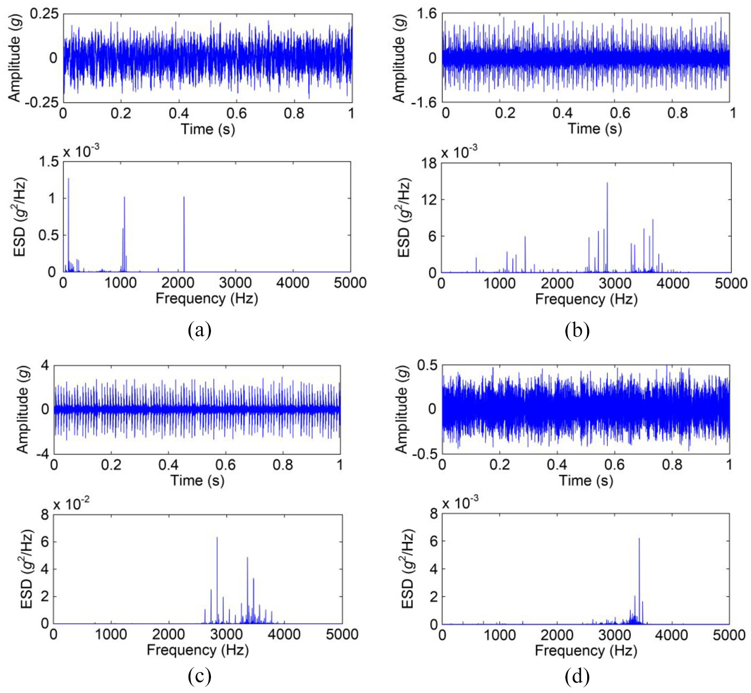
Time domain waveform and energy spectral density of bearing vibration signals of the four operation states: (a) normal, (b) inner race fault, (c) outer race fault, and (d) rolling ball fault.

It can be easily seen from Figure 7 that the time domain waveforms of bearing vibration signals of the four operation states are complex and hard to distinguish, while the corresponding ESDs of that are simple and easy to distinguish. The ESDs clearly illustrate the energy distribution characters of bearing vibration signals of the four operation states, respectively. In the frequency domain, the effective components of each bearing vibration signal are greatly different, and meantime the dominant components of the four bearing vibration signals appear at the different frequency. And consequently, the energy values in the different frequency bands of each vibration signal are bound to be different. It is also demonstrated energy is certainly a powerful index for measuring different bearing operation states. Moreover, the various waveforms and ESDs also make the kurtosis of the different faults diverse.

Usually, the raw vibration data can hardly be used for fault identification directly, so the preprocessing is necessary. For each raw vibration data sample of CWRU, one operation state only has one data sample and there are a large number of sampling points in one sample. In order to achieve intelligent fault identification via the proposed method, each raw vibration data sample was divided into more samples by resampling scheme. The number of resampling points is 6000 for each new data sample, and each raw vibration data sample can form 20 new data samples, so the resampled vibration dataset including four operation states of the rolling bearing consists of 20 × 4 new data samples.

Subsequently, the vibration signal dataset formed above was processed through the proposed method to identify the four operation states of the bearing. In the first step, five IMFs can be derived from each sample by using VMD technique, and the obtained IMFs of the bearing vibration signals of the four operation states are shown in Figure 8.

Figure 8.

IMFs of bearing vibration signals of the four operation states processed by VMD: (a) normal, (b) Inner race fault, (c) outer race fault, and (d) rolling ball fault.

It can be observed from Figure 8 that there are some differences in the decomposition results of the bearing vibration signals of the four operation states processed by VMD. The waveforms of all IMFs are obviously different, and each IMF represents a particular vibration component. The results indicate that the VMD method can effectively decompose the bearing vibration signal into a series of sub-signals with different vibration characteristics.

On the basis of the decomposed results, the energy (En) and kurtosis (Ku) of each IMF can be computed. And consequently, 10 fault features have been obtained for each fault data sample. The energy and kurtosis values of all IMFs of 80 data samples obtained from four operation states are shown in Table 1.

Table 1.

Energy and kurtosis values of five IMFs of each data sample.

Data samples	IMF1		IMF2		IMF3		IMF4		IMF5		Operationstates
Data samples	En1	Ku1	En2	Ku2	En3	Ku3	En4	Ku4	En5	Ku5	Operationstates
1	1.51 × 10⁻³	2.78	1.44 × 10⁻³	2.83	5.49 × 10⁻⁴	1.58	2.91 × 10⁻⁶	2.97	2.80 × 10⁻⁶	3.26	N
…	…	…	…	…	…	…	…	…	…	…
20	1.74 × 10⁻³	2.72	1.37 × 10⁻³	2.90	5.36 × 10⁻⁴	1.60	3.01 × 10⁻⁶	2.90	3.08 × 10⁻⁶	2.94
21	1.84 × 10⁻³	2.29	4.20 × 10⁻³	2.78	1.00 × 10⁻²	3.96	5.18 × 10⁻³	3.70	8.95 × 10⁻³	3.91	IF
…	…	…	…	…	…	…	…	…	…	…
40	2.01 × 10⁻³	2.23	4.22 × 10⁻³	2.75	1.02 × 10⁻²	4.02	5.02 × 10⁻³	3.93	8.81 × 10⁻³	4.06
41	6.64 × 10⁻⁴	2.81	6.78 × 10⁻⁴	2.90	3.64 × 10⁻²	4.10	7.77 × 10⁻²	5.13	1.35 × 10⁻³	8.31	OF
…	…	…	…	…	…	…	…	…	…	…
60	6.88 × 10⁻⁴	2.99	7.17 × 10⁻⁴	2.97	3.69 × 10⁻²	4.00	7.62 × 10⁻²	5.33	1.62 × 10⁻³	9.34
61	2.14 × 10⁻⁴	2.96	1.74 × 10⁻⁴	3.09	1.06 × 10⁻³	3.15	2.57 × 10⁻³	2.36	3.19 × 10⁻³	2.49	RF
…	…	…	…	…	…	…	…	…	…	…
80	2.01 × 10⁻⁴	2.94	1.77 × 10⁻⁴	3.19	1.08 × 10⁻³	3.33	2.64 × 10⁻³	2.65	3.56 × 10⁻³	2.14

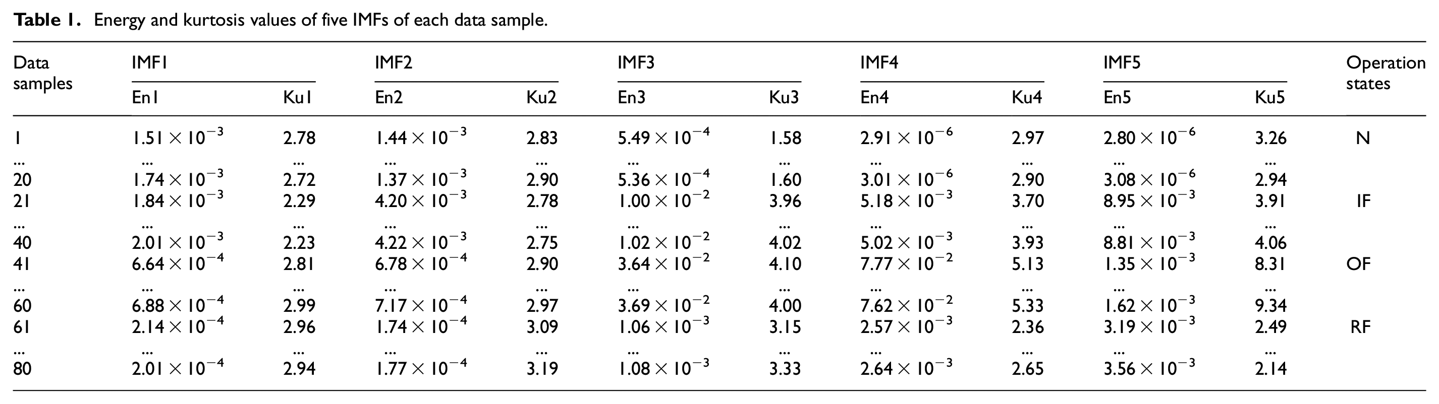
It can be easily found from Table 1 that the values of the quantitative fault features (i.e. energy and kurtosis) derived from some of IMFs are largely different. Actually, this situation may lead to the large errors while data compression is performed. In order to decrease the numerical difference between any two fault features, the energy and kurtosis values were normalized and scaled into the interval [0, 1]. That is, each column of quantitative fault features in Table 1 was conducted through the following equation:

y = \frac{x - x_{min}}{x_{max} - x_{min}}

(25)

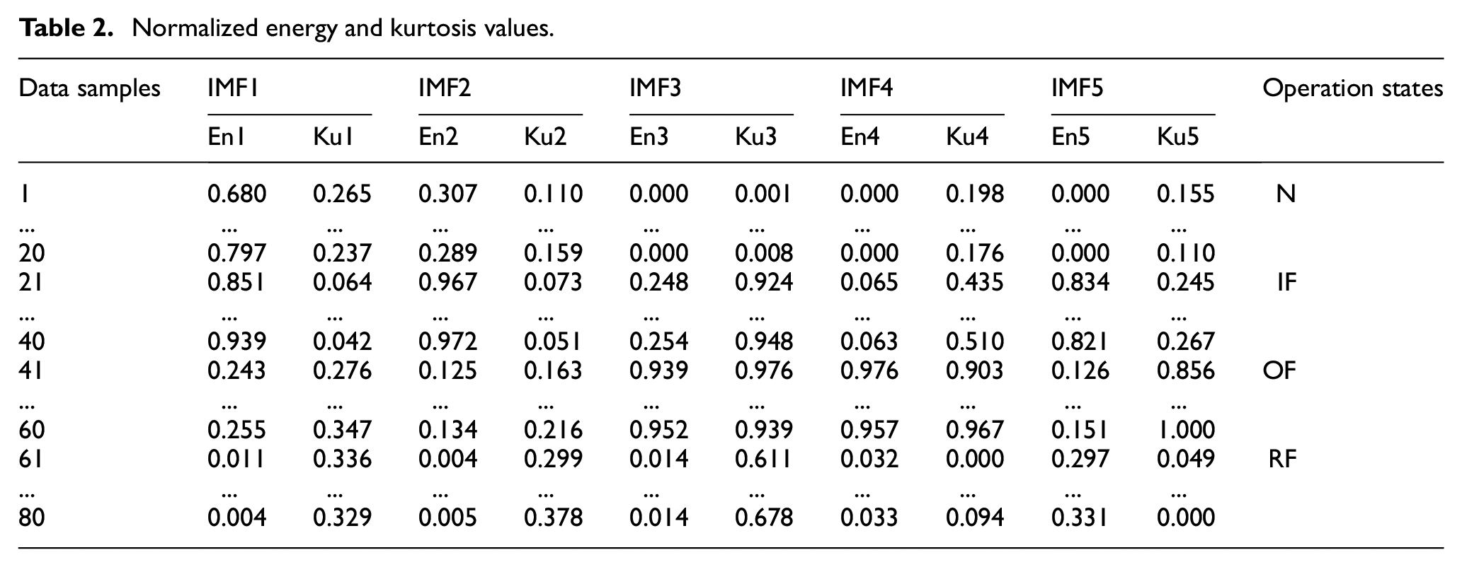
where x and y are the original data value and the corresponding value after normalization of each feature respectively, and x_max and x_min are the maximum and minimum values in the same column of Table 1 respectively. The normalized energy and kurtosis values are shown in Table 2.

Table 2.

Normalized energy and kurtosis values.

Data samples	IMF1		IMF2		IMF3		IMF4		IMF5		Operation states
Data samples	En1	Ku1	En2	Ku2	En3	Ku3	En4	Ku4	En5	Ku5	Operation states
1	0.680	0.265	0.307	0.110	0.000	0.001	0.000	0.198	0.000	0.155	N
…	…	…	…	…	…	…	…	…	…	…
20	0.797	0.237	0.289	0.159	0.000	0.008	0.000	0.176	0.000	0.110
21	0.851	0.064	0.967	0.073	0.248	0.924	0.065	0.435	0.834	0.245	IF
…	…	…	…	…	…	…	…	…	…	…
40	0.939	0.042	0.972	0.051	0.254	0.948	0.063	0.510	0.821	0.267
41	0.243	0.276	0.125	0.163	0.939	0.976	0.976	0.903	0.126	0.856	OF
…	…	…	…	…	…	…	…	…	…	…
60	0.255	0.347	0.134	0.216	0.952	0.939	0.957	0.967	0.151	1.000
61	0.011	0.336	0.004	0.299	0.014	0.611	0.032	0.000	0.297	0.049	RF
…	…	…	…	…	…	…	…	…	…	…
80	0.004	0.329	0.005	0.378	0.014	0.678	0.033	0.094	0.331	0.000

In order to extract the imbedded information of bearing faults and obtain more sensitive fault features, the fault dataset shown in Table 2 was conducted via PCA. For comparison, VMD method was replaced with EMD method in the above procedures. Consequently, two groups of principal components can be produced, and their contribution rates are shown in Figure 9.

Figure 9.

Contribution rates and cumulative contribution rates of PCs originated from (a) VMD and (b) EMD.

It can be seen from Figure 9 that the contribution rates of the first several PCs respectively originated from VMD and EMD are much different. The contribution rates of the first three PCs originated from VMD are obviously larger than that from EMD. And consequently, the cumulative contribution rate of the first three PCs originated from VMD is also larger than that from EMD. The former already exceeds 95%, but the latter does not reach 60%. To more clearly illustrate the distinctions of two different groups of PCs in Figures 9(a) and (b), the distributions of the first three PCs respectively originated from VMD and EMD are shown in Figure 10.

Figure 10.

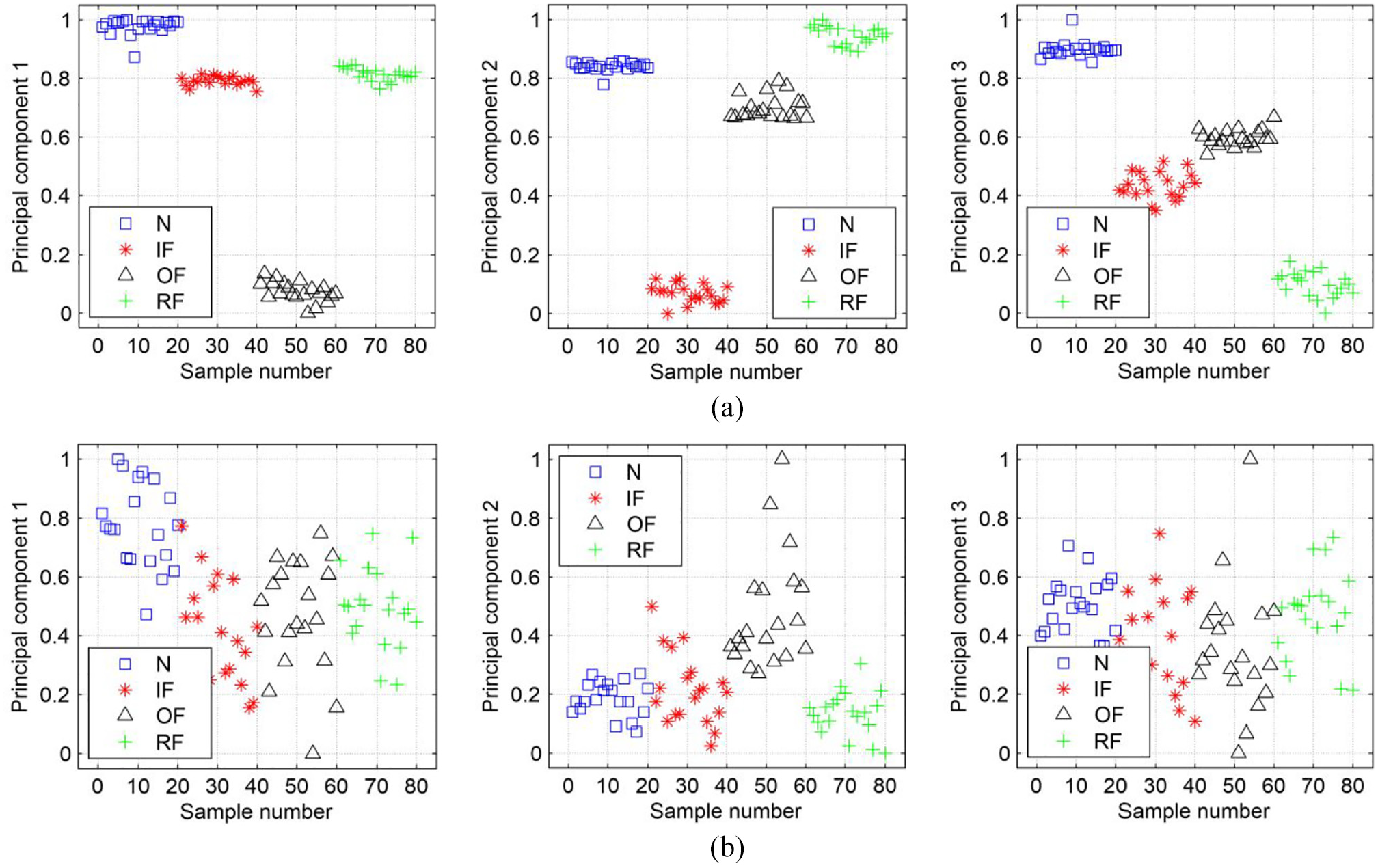
Distribution of the first three PCs originated from (a) VMD and (b) EMD.

As can be seen from Figure 10, the distribution of the first three PCs originated from VMD is clustered and distinct for the four operation states, while that originated from EMD is dispersed and overlapped. Therefore, the first three PCs originated from VMD retain most of useful original information of different operation states.

Next, the two groups of PCs whose cumulative contribution rate is above 85% in Figure 9 were respectively input into the designed SVMDT for data classification and bearing fault identification. For each operation state, the data samples were randomly divided into two parts. One part, 75% of the data samples, was selected randomly as the training samples, and the other, the remaining 25%, as the testing samples. In order to ensure effectiveness and accuracy of the fault identification results, we repeated this procedure 10 times, and used the average accuracies of the classification results as the metric. This conduction is similar to 10-fold cross-validation scheme. Meanwhile, a typical deep learning model, one-dimensional convolutional neural network (1DCNN), was also applied to fault identification. The classification results of the three methods are shown in Table 3.

Table 3.

Classification results of the three methods.

Methods	Training accuracies	Testing accuracies	Time consumption
VMD + PCA-SVM	100%	98.6%	263 s
EMD + PCA-SVM	100%	84.5%	759 s
1DCNN	61.3%	62.9%	316 s

From Table 3, it is clearly found that the former two methods have the same training accuracy and relatively high testing accuracy, but the method, 1DCNN, has the lowest training and testing accuracies. Besides, the proposed method, VMD + PCA-SVM, consumes the least computation time. These results indicate that the first method, under the condition of small samples, provides better generalization performance and higher computation efficiency than the latter two methods in fault data classification. Because the classification accuracy of 1DCNN is overly low, it is no longer studied in the follows. A testing result of bearing fault identification, when VMD + PCA-SVM and EMD + PCA-SVM obtained the best testing accuracies respectively, is shown in Figure 11.

Figure 11.

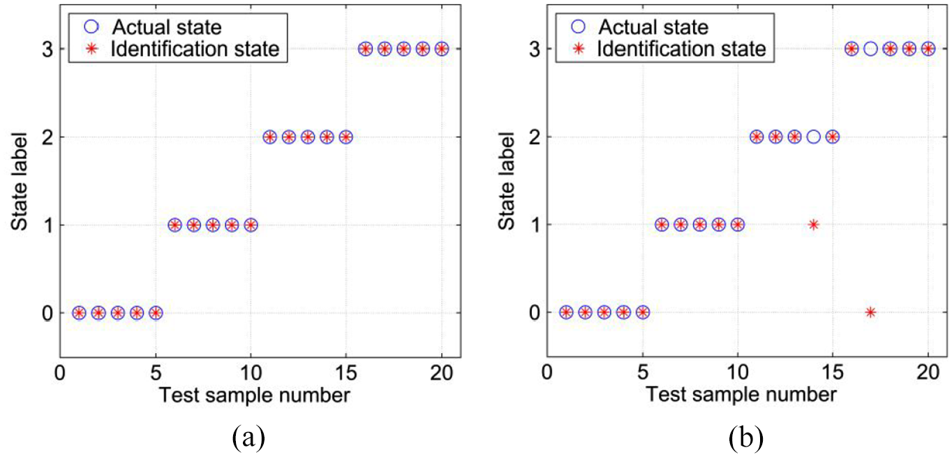
A testing result of bearing fault identification: (a) VMD + PCA-SVM and (b) EMD + PCA-SVM.

As shown in Figure 11, the state labels “0,”“1,”“2,” and “3” along vertical axis represent normal, inner race fault, outer race fault, and rolling ball fault, respectively. It can be easily seen that the VMD + PCA-SVM method can identify the four operation states correctly, while the EMD + PCA-SVM method is unable to correctly recognize two test data samples. In other words, the former method can achieve the highest fault recognition accuracy of 100%, while the highest fault recognition accuracy of the latter method only reaches 90%. This is because the VMD method can more accurately decompose the bearing vibration signals and effectively extract the fault features, which also can be observed from the illustrations in Figures 9 and 10.

Moreover, to further effectively illustrate the difference between the classification results of the two methods, we used the first two PCs respectively shown in Figure 9(a) and (b) as the input features for fault data classification. And subsequently, these data samples were handled through the SVMDT algorithm. After completion of the fault data classification, Figure 12 gives the visual classification processes and results of the four operation states of the rolling bearing.

Figure 12.

Visual classification results of the four operation states of the rolling bearing with the first two PCs originated from VMD and EMD: (a) binary classification process of VMD + PCA-SVM and (b) binary classification process of EMD + PCA-SVM.

As shown in Figure 12, the fault data samples of four operation states of the rolling bearing can be gradually identified using the SVMDT algorithm (the identification order is OF, IF, RF, and N). Comparing with Figure 12(a) and (b), it can be clearly seen that the first two PCs of the fault data samples of the rolling bearing originated from VMD are more easily distinguishable than that from EMD. Moreover, according to Figure 9, it is obvious that the cumulative contribution rate of the first two PCs originated from VMD exceeds 80%, but that from EMD merely exceeds 40%. Thus, the former carries most of useful information of four operation states of the rolling bearing, so the margins between the decision boundaries of the SVMDT model for fault data classification are wide. In contrast, the latter only has little useful information, and the corresponding margins are narrow. All these cause that the former method, VMD combined with PCA-SVM, can extract important fault features more effectively and identify incipient faults of rolling bearings more accurately than the latter method, EMD combined with PCA-SVM. It is definitely demonstrated through this validation experiment that the proposed method can achieve the accurate and intelligent identification of incipient rolling bearing faults.

Case study 2

In order to validate the generalization and robustness of the proposed method, an experiment was implemented on the bearing test rig shown in Figure 13. As can be seen, the bearing test rig is different from the CWRU bearing test rig more or less, and the four elements marked in Figure 13 have the same functions as corresponding elements of the CWRU bearing test rig.

Figure 13.

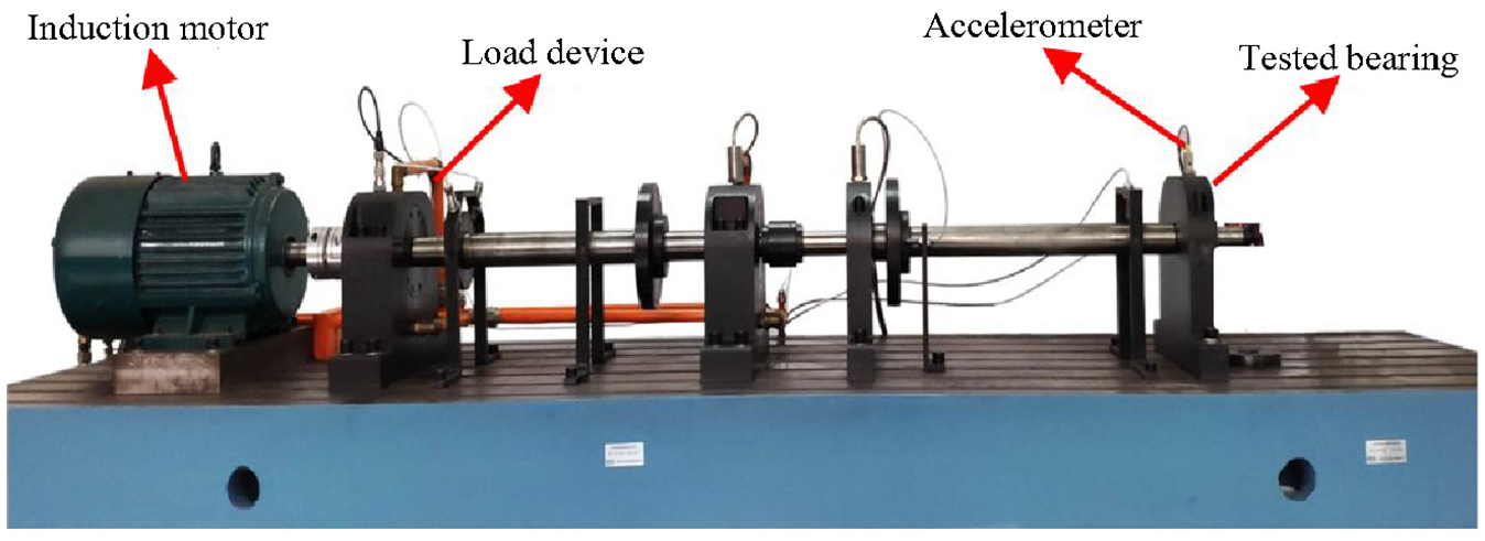
A typical rolling bearing test rig.

In this experiment, we selected NSK 6308 rolling bearing as the tested bearing and five kinds of operation states of the bearing were considered. The operation states include normal (N), inner race fault (IF), outer race fault (OF), rolling ball fault (RF), and cage fault (CF). Moreover, the four kinds of faults were machined through the electro-discharge machining and the fault defects were very tiny and slight. To keep the comparability, the outer race fault also was located at 6 o’clock, which is the same setting as case study 1. The vibration signals of five kinds of operation states were acquired at the rotational speed of 2800 r/min and the sampling frequency was set as 8 kHz. In this condition, if the data sampling time lasts 0.5 s, the inner race of the bearing can rotate about 23 rounds which are adequate for bearing fault analysis. So, 4096 sampling points were collected for each data sample, of which the sampling time is equal to 0.512 s.

For each operation state of the bearing, we collected 40 vibration data samples. As five kinds of operation states of the bearing were considered, the bearing fault dataset was composed of 40 × 5 vibration data samples. And subsequently, the fault dataset was conducted by using the three methods which had been applied to the CWRU bearing fault dataset for fault recognition. Since the processing procedures of this fault dataset are the same as that of the fault dataset in case study 1, here we describe no more details of the processing procedures and only show the ultimate fault classification results. The classification results of the fault dataset are shown in Table 4.

Table 4.

Classification results of the fault dataset by using three methods.

Methods	Training accuracies	Testing accuracies	Time consumption
VMD +PCA-SVM	100%	99.1%	429 s
EMD + PCA-SVM	99.8%	86.3%	1641 s
1DCNN	70.2%	66.4%	587 s

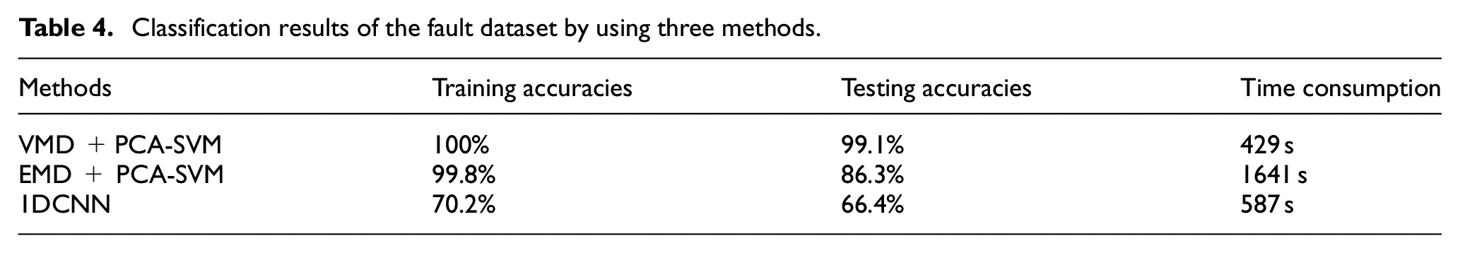
Compared Table 4 with Table 3, it can be found that the classification results in Table 4 are very similar to that in Table 3. The proposed method, VMD + PCA-SVM, still has the highest classification accuracies and consumes the least time in the whole process of fault data pattern recognition. The latter two methods have lower classification accuracies and more time consumption. Besides, the method, 1DCNN, maintains the lowest training and testing accuracies, although the number of data samples becomes double. These results also verify that the proposed method, under the condition of small samples, actually can provide better generalization performance and higher computation efficiency, and deep learning model hardly has any superiority. So, in the next part, there is no need to show the identification results of 1DCNN. A best recognition result of bearing faults, obtained by employing VMD + PCA-SVM and EMD + PCA-SVM respectively, is shown in Figure 14.

Figure 14.

A best recognition result of bearing faults: (a) VMD + PCA-SVM and (b) EMD + PCA-SVM.

As shown in Figure 14, the state labels “0,”“1,”“2,”“3,” and “4” along vertical axis represent five kinds of operation states: N, IF, OF, RF, and CF, respectively. The result clearly illustrates that the VMD + PCA-SVM method can accurately classify five kinds of bearing operation states, while the EMD + PCA-SVM method has no ability to correctly identify four test data samples. It is indicated that the proposed method can also reach a higher fault recognition rate, and the best recognition rate of the other method still doesn’t exceed 90%. By comparing Figures 11(b) and 14(b), it can be easily found that the normal and inner race fault always can be correctly identified, while a few data samples of the rest of the operation states cannot be correctly recognized. These results verify that EMD, compared with VMD, really has no superiority in bearing signal decomposition and fault feature extraction, which is consistent with the result in case study 1. And therefore, VMD definitely plays a greatly important role in our proposed method for bearing fault identification.

Discussion

Fault diagnosis technology is very important for guaranteeing the safe operation of mechanical equipment. An effective fault diagnosis method not only can be employed to fault detection, identification, and prognosis in the operational process of rotating machinery, but also can extremely promote work efficiency and economic benefits. At present, vibration analysis is still a most effective fault diagnosis method because of its high accuracy. Frequency spectrum can be obtained by implementing Fourier transform on vibration signals, and then the characteristic frequency of the corresponding fault can be found for further analysis. Actually, time-frequency analysis is more suitable for processing the vibration signals of rotating machinery. More useful fault information can be obtained from the vibration signals, so time-frequency analysis is better than frequency spectrum analysis. However, both of them greatly depend on the experience of fault diagnosis experts, so they are not convenient for site operators. Machine learning method is a kind of data-driven artificial intelligence method, so it is more intuitive in the field of intelligent fault diagnosis. Because quantitative feature extraction and automatic classification are two key steps to machine learning, how to achieve the accurate fault feature extraction and fault data classification become the most important works for the incipient fault intelligent identification of rolling bearings. Although some common methods have no outstanding performance, they can perform very well when integrated. So, this is really a promising way to improve the diagnosis accuracy and efficiency.

After analyzing the advantages and disadvantages of above methods, we decide to carry out incipient fault recognition of rolling bearings by analyzing vibration signals and developing an intelligent diagnosis method based on VMD and PCA-SVM. And, in this method, two simple quantitative fault features (energy and kurtosis) are extracted. The excellent performance of the method is verified through two bearing fault datasets and the comparative analysis. Moreover, this method also can be applied to fault detection and diagnosis of other rotating machinery equipment, not just the incipient fault diagnosis of rolling bearings. In our future works, we will verify the effectiveness of the proposed method on typical rotating machinery (such as gearbox, bearing-rotor system, centrifugal pump, as shown in Figure 15), and optimize the parameters of the proposed method in engineering application to improve its performance.

Figure 15.

Typical rotating machinery that can be diagnosed by using the proposed method: (a) gearbox and bearing-rotor system and (b) centrifugal pump.

Conclusions

In this paper, we propose a new incipient fault intelligent identification method of rolling bearings based on variational mode decomposition, principal component analysis, and support vector machines. In this method, we use VMD to decompose the raw vibration signals of rolling bearings into a group of IMFs, and then the energy and kurtosis of these IMFs are computed. Although this conduction is a general processing step, the most useful fault feature information can be effectively extracted from the raw vibration signals. After that, PCA and SVM are combined and employed to achieve bearing fault identification. The parameters of VMD and SVM are set according to the previous research results. And finally, we test our proposed method on Case Western Reserve University bearing fault dataset and an experimental bearing fault dataset. The results of the validation experiment concretely show that VMD based quantitative fault features of different fault types have obvious distinctions and good separability, and the proposed method can achieve accurate identification of the rolling bearing incipient faults. By comparative analyses of our proposed method and other two methods (i.e. EMD + PCA-SVM and 1DCNN), the superior performance of our proposed method is further demonstrated. Compared with EMD + PCA-SVM and 1DCNN, our proposed method can more accurately and efficiently identify the incipient faults of rolling bearings. In case study 1, the average identification accuracy reaches 98.6% and the average time consumption is only 263 s of our proposed method. In contrast, EMD + PCA-SVM and 1DCNN only have the accuracy of 84.5% and 62.9% but takes 759 and 316 s. In case study 2, our proposed method still outperforms other two methods obviously. The identification accuracy and the computation time of the three methods (i.e. VMD + PCA-SVM, EMD + PCA-SVM, and 1DCNN) are 99.1%, 86.3%, 66.4% and 429, 1641, 587 s, respectively.

The proposed method can be employed to implement vibration signal analysis and fault diagnosis of any rotating mechanical equipment, not just rolling bearings. And this method is extremely suitable to process the small sample data. In future research, we will further study the application of the proposed method for the intelligent fault recognition of other mechanical equipment, and design an algorithm that can effectively search the optimal parameters of the proposed method according to the practical fault diagnosis problem of rotating machinery.

Footnotes

Acknowledgements

We sincerely thank Professor Kenneth A. Loparo and Case Western Reserve University Bearing Data Center for supplying fault bearing dataset, and the anonymous reviewers for their constructive suggestions to improve the quality of this paper.

Handling Editor: Chenhui Liang

Declaration of conflicting interests

The author(s) declared no potential conflicts of interest with respect to the research, authorship, and/or publication of this article.

Funding

The author(s) disclosed receipt of the following financial support for the research, authorship, and/or publication of this article: This research was funded by the China Postdoctoral Science Foundation (grant number 2016M592857) and the Natural Science Foundation of Gansu Province (grant number 1610RJZA004).

ORCID iD

Linfeng Deng

References

Yang

Chen

Effects of rolling bearing configuration on stiffness of machine tool spindle. Proc Inst Mech Eng Part C: J Mech Eng Sci 2018; 232: 775–785.

Qiao

Pan

SVD principle analysis and fault diagnosis for bearings based on the correlation coefficient. Meas Sci Technol 2015; 26: 085014.

Zhang

, et al. Intelligent fault diagnosis of rolling bearings using variational mode decomposition and self-organizing feature map. J Vib Control 2020; 26: 1886–1897.

Xiong

Zhou

, et al. A novel end-to-end fault diagnosis approach for rolling bearings by integrating wavelet packet transform into convolutional neural network structures. Sensors 2020; 20: 4965.

Wang

A sparse underdetermined blind source separation method and its application in fault diagnosis of rotating machinery. Complexity 2020; 2020: 2428710.

Liu

Chen

. Research on bearing fault feature extraction based on singular value decomposition and optimized frequency band entropy. Mech Syst Sig Process 2019; 118: 477–502.

Al-Bugharbee

Trendafilova

A fault diagnosis methodology for rolling element bearings based on advanced signal pretreatment and autoregressive modelling. J Sound Vib 2016; 369: 246–265.

Sun

Liao

Lin

The shock pulse index and its application in the fault diagnosis of rolling element bearings. Sensors 2017; 17: 535.

Lei

Lin

, et al. A review on empirical mode decomposition in fault diagnosis of rotating machinery. Mech Syst Signal Process 2013; 35: 108–126.

10.

Gilles

Empirical wavelet transform. IEEE Trans Signal Process 2013; 61: 3999–4010.

11.

Dragomiretskiy

Zosso

Variational mode decomposition. IEEE Trans Signal Process 2014; 62: 531–544.

12.

Jiang

Zhu

An improved VMD with empirical mode decomposition and its application in incipient fault detection of rolling bearing, IEEE Access 2018; 6: 44483–44493.

13.

Deng

Zhao

, et al. A novel rolling bearing fault diagnosis method based on empirical wavelet transform and spectral trend. IEEE Trans Instrum Meas 2020; 69: 2891–2904.

14.

Hoang

Kang

HJ.

A survey on deep learning based bearing fault diagnosis. Neurocomputing 2019; 335: 327–335.

15.

Niu

Wang

Golda

, et al. An optimized adaptive PReLU-DBN for rolling element bearing fault diagnosis. Neurocomputing 2021; 445: 26–34.

16.

Jiang

Cheng

A novel method for adaptive multiresonance bands detection based on VMD and using MTEO to enhance rolling element bearing fault diagnosis. Shock Vib 2016; 2016: 8361289.

17.

, et al. A rolling bearing fault diagnosis method based on variational mode decomposition and an improved kernel extreme learning machine. Appl Sci 2017; 7: 1004.

18.

Wang

Incipient fault feature extraction of rolling bearings based on the MVMD and Teager energy operator. ISA Trans 2018; 80: 297–311.

19.

Zhang

Jiang

Feng

Research on variational mode decomposition in rolling bearings fault diagnosis of the multistage centrifugal pump. Mech Syst Signal Process 2017; 93: 460–493.

20.

Chen

Hao

, et al. Weak fault detection method of rolling bearing based on testing signal far away from fault source. J Mech Sci Technol 2020; 34: 1035–1048.

21.

Zheng

Zhou

, et al. Application of variational mode decomposition and permutation entropy for rolling bearing fault diagnosis. Int J Acoust Vib 2019; 24: 303–311.

22.

Ding

Huang

Xiao

, et al. GMPSO-VMD algorithm and its application to rolling bearing fault feature extraction. Sensors 2020; 20: 1946.

23.

Gai

Shen

, et al. An integrated method based on hybrid grey wolf optimizer improved variational mode decomposition and deep neural network for fault diagnosis of rolling bearing. Measurement 2020; 162: 107901.

24.

Zhou

, et al. Early fault feature extraction of bearings based on Teager energy operator and optimal VMD. ISA Trans 2019; 86: 249–265.

25.

Yan

Jia

Intelligent fault diagnosis of rotating machinery using improved multiscale dispersion entropy and mRMR feature selection. Knowl Based Syst 2019; 163: 450–471.

26.

Jin

Han

Zhang

, et al. An intelligent fault diagnosis method of rolling bearings based on Welch power spectrum transformation with radial basis function neural network. J Vib Control 2020; 26: 629–642.

27.

Liang

Deng

, et al. Intelligent fault diagnosis via semisupervised generative adversarial nets and wavelet transform. IEEE Trans Instrum Meas 2020; 69: 4659–4671.

28.

Seghouane

Shokouhi

Koch

Sparse principal component analysis with preserved sparsity pattern. IEEE Trans Image Process 2019; 28: 3274–3285.

29.

Guo

Wang

Granular support vector machine: a review. Artif Intell Rev 2019; 51: 19–32.

30.

Faisal

A data-driven principal component analysis-support vector machine approach for breast cancer diagnosis: comparison and application. Trans Inst Meas Control 2020; 42: 1301–1312.

31.

Fan

Cui

Han

, et al. Chiller fault diagnosis with field sensors using the technology of imbalanced data. Appl Therm Eng 2019; 159: 113933.

32.

Monroy

Benitez

Escudero

, et al. Enhanced plant fault diagnosis based on the characterization of transient stages. Comput Chem Eng 2012; 37: 200–213.

33.

Onel

Kieslich

Pistikopoulos

EN.

A nonlinear support vector machine-based feature selection approach for fault detection and diagnosis: application to the Tennessee Eastman process. AIChE J 2019; 65: 992–1005.

34.

Wang

Liu

Bao

, et al. Stacked sparse autoencoder with PCA and SVM for data-based line trip fault diagnosis in power systems. Neural Comput Appl 2019; 31: 6719–6731.

35.

Zhou

, et al. Fault diagnosis method of rolling bearing using principal component analysis and support vector machine. J Mech Sci Technol 2018; 32: 5079–5088.

36.

Fan

Zhou

, et al. A wavelet-based statistical approach for monitoring and diagnosis of compound faults with application to rolling bearings. IEEE Trans Autom Sci Eng 2018; 15: 1563–1572.

37.

Wang

Zheng

Rolling element bearings fault diagnosis based on a novel optimal frequency band selection scheme. IEEE Access 2019; 7: 80748–80766.

38.

Cheng

Chen

Wang

Clustering of the body shape of the adult male by using principal component analysis and genetic algorithm–BP neural network. Soft Comput 2020; 24: 13219–13237.

39.

Chauhan

Dahiya

Sharma

Problem formulations and solvers in linear SVM: a review. Artif Intell Rev 2019; 52: 803–855.

40.

Srinivas

Srinivasan

Umesh

KN.

Role of an artificial neural network and a wavelet transform for condition monitoring of the combined faults of unbalance and cracked rotors. Int J Acoust Vib 2010; 15: 121–127.

41.

Zair

Rahmoune

Benazzouz

Multi-fault diagnosis of rolling bearing using fuzzy entropy of empirical mode decomposition, principal component analysis, and SOM neural network. Proc Inst Mech Eng Part C J Mech Eng Sci 2019; 233: 3317–3127.

42.

Babouri

Djebala

Ouelaa

, et al. Rolling bearing faults severity classification using a combined approach based on multi-scales principal component analysis and fuzzy technique. Int J Adv Manuf Technol 2020; 107; 4301–4316.

43.

Wang

Chen

, et al. Research on rolling bearing state health monitoring and life prediction based on PCA and internet of things with multi-sensor. Measurement 2020; 157: 107657.

44.

Teng

Zhu

, et al. SVM-DT-based adaptive and collaborative intrusion detection. IEEE-CAA J Autom Sin 2018; 5: 108–118.

45.

Yan

Jia

A novel optimized SVM classification algorithm with multi-domain feature and its application to fault diagnosis of rolling bearing. Neurocomputing 2018; 313: 47–64.

46.

Tharwat

Parameter investigation of support vector machine classifier with kernel functions. Knowl Inf Syst 2019; 61: 1269–1302.

47.

Loparo

KA.

Case Western Reserve University bearing data center seeded fault test data, Available online: http://csegroups.case.edu/bearingdatacenter/pages/download-data-file (2003, accessed 30 May 21).

Intelligent identification of incipient rolling bearing faults based on VMD and PCA-SVM

Abstract

Keywords

Introduction

Related basic theories

Variational mode decomposition

Signal energy and kurtosis

Principal component analysis and support vector machine

Proposed method

Experimental results

Case study 1

Case study 2

Discussion

Conclusions

Footnotes

Acknowledgements

Declaration of conflicting interests

Funding

ORCID iD

References