Sage Journals: Discover world-class research

Abstract

As wheels are important components of train operation, diagnosing and predicting wheel faults are essential to ensure the reliability of rail transit. Currently, the existing studies always separately deal with two main types of wheel faults, namely wheel radius difference and wheel flat, even though they are both reflected by wheel radius changes. Moreover, traditional diagnostic methods, such as mechanical methods or a combination of data analysis methods, have limited abilities to efficiently extract data features. Deep learning models have become useful tools to automatically learn features from raw vibration signals. However, research on improving the feature-learning capabilities of models under noise interference to yield higher wheel diagnostic accuracies has not yet been conducted. In this paper, a unified training framework with the same model architecture and loss function is established for two homologous wheel faults. After selecting deep residual networks (ResNets) as the backbone network to build the model, we add the squeeze and excitation (SE) module based on a multichannel attention mechanism to the backbone network to learn the global relationships among feature channels. Then the influence of noise interference features is reduced while the extraction of useful information features is enhanced, leading to the improved feature-learning ability of ResNet. To further obtain effective feature representation using the model, we introduce supervised contrastive loss (SCL) on the basis of ResNet + SE to enlarge the feature distances of different fault classes through a comparison between positive and negative examples under label supervision to obtain a better class differentiation and higher diagnostic accuracy. We also complete a regression task to predict the fault degrees of wheel radius difference and wheel flat without changing the network architecture. The extensive experimental results show that the proposed model has a high accuracy in diagnosing and predicting two types of wheel faults.

Keywords

Fault diagnosis wheel faults ResNet multichannel attention supervised contrastive learning

Introduction

In recent years, rail transportation business has developed rapidly in China, but the safety situation is increasingly serious, and guaranteeing the reliability of the rail system is still the top priority of the rail transportation business.¹ Though the research related to rail vehicle fault diagnosis has been carried out to an increasing extent in China, a preventive maintenance method for overhauling trains is mostly adopted. If the operation status of key train components can be monitored, the transformation to a condition-based maintenance will be achieved to fulfill the requirements of reliability, availability, maintainability, and safety (RAMS).

For the fault diagnosis and condition monitoring of trains, the faulting of key equipment is the biggest threat to the safe operation of rail vehicles, so studying the key equipment, such as bearings and wheels in train operation, has become the top priority of fault diagnosis.^2,3 Currently, bearing faults have been diagnosed in depth,^4–6 but the wheel, as an important component, is rarely examined in fault diagnosis. One characteristic of a wheel is that it is in contact with the track, making it subject to enormous friction and wheel gravity forces. Thus, wheels wear severely, and fault diagnosis is particularly important.

One of the most common forms of wheel faults is wheel radius difference. When the train turns, the outer wheel wears more seriously, and the radius of the wheel that is more often on the outer side is reduced. The existence of wheel radius difference can change the alignment balance position of the wheel pair and affect the stability and safety of the vehicle system.⁷ Another common form of wheel faults is wheel flat, which refers to a situation wherein a section of the wheel arc is out of round. When the train undergoes starting, braking, or sudden acceleration and deceleration often, a part of the wheel may disappear due to severe wear. The wheel flat causes the contact areas between the wheel and the rail to become larger, resulting in wheel vibration and derailment.⁸ However, previous studies^7–11 always dealt with the two forms of wheel faults separately. In fact, wheel radius difference and wheel flat are both reflected in wheel radius changes. We consider integrating two homologous faults into a training framework with the same model architecture and loss function. When the input is from a wheel pair, the model for wheel radius difference can be trained. When the input is from a single wheel, the model for wheel flat can be obtained.

For these two forms of wheel faults, traditional diagnosis methods, such as mechanical methods or a combination of data analysis methods, have limited ability to efficiently extract data features. Deep learning models with multilevel nonlinear transformations have become useful tools for automatically learning features from raw vibration signals. Different from convolutional neural network (CNN), deep residual network (ResNet) proposed by He et al.¹² introduces the identity shortcut, which provides a direct channel for gradient propagation and alleviates the difficulty of parameter optimization; therefore, this network was selected as the backbone network to build the model.

However, the interference of noise often exists in vibration signals, leading to the degradation of the ability of models to obtain effective feature representations. The squeeze and excitation (SE)¹³ module can learn global information relationships among feature channels, so it was added to the backbone network to improve the feature-learning ability of ResNet under noise interference. By setting appropriate filters on the signals according to global relationships, the influence of noisy interference features can be reduced and the ability to extract useful information from the signals can be enhanced.

Furthermore, improving feature-learning capability is an important task for deep learning models when applied to fault diagnosis. Although the cross-entropy loss function is the most widely used loss function in supervised classification models, it has the characteristics of poor robustness to noise labels and weak generalization ability. Recently, contrastive loss function^14,15 has been studied to implement feature representation and pretraining for downstream tasks. However, most studies have focused on self-supervised representation learning without labels. That is, only positive examples are obtained by data augmentation of the anchor sample, while the remaining samples in the dataset are treated as negative examples. Therefore, there is a high probability that such negative examples contain samples belonging to the same class as the anchor sample, resulting in the “false negative samples” phenomenon. This phenomenon is an obstacle to obtaining effective feature representation because of the distancing of the positive examples from “false negative samples.” To exploit the labels of our fault training samples, inspired by the idea of Khosla et al.,¹⁶ we introduce supervised contrastive loss (SCL) for training. With the guidance of label information, positive and negative samples are accurately identified and the phenomenon of “false negative samples” is eliminated, resulting in better feature representation.

Based on this method, we use supervised contrastive learning on the basis of ResNet + SE to increase the feature distances of different fault classes through a comparison between positive and negative examples under the supervision of label information, so that better category differentiation and higher fault diagnosis accuracy can be achieved. The experimental data is generated from German side by using the multibody dynamics (MBD) software SIMPACK to simulate fault damages. The contributions of this study are summarized as follows:

We establish a unified training framework with the same model architecture and loss function for both wheel radius difference and wheel flat.

We improve the feature-learning capability and noise robustness of the model by adding the multichannel attention SE module and introducing supervised contrastive loss.

We also complete the regression task to predict the fault degrees of wheel radius difference and wheel flat without changing the model network architecture.

The rest of this paper is organized as follows. Section 2 describes the related work. The fault diagnosis and prediction system is presented in detail in Section 3. Section 4 describes the experimental parameters and results. Finally, conclusions are given in Section 5.

Related work

Train wheel fault-diagnostic methods can be broadly classified into two categories: traditional methods and deep-learning-based methods, as shown in Table 1.

Table 1.

List of popular techniques for fault feature extraction.

Category	Techniques
Time-domain analysis	Statistics¹⁷ Time synchronous average (TSA)¹⁸ Autoregressive moving average (ARMA)¹⁹ Principal component analysis (PCA)²⁰ Correlation-based analysis²¹
Frequency-domain analysis	Fast Fourier transform (spectrum analysis)²² Hilbert transform (envelope analysis)^8,23 Inverse Fourier Transform of logarithmic power spectrum (cepstrum analysis)²⁴
Time-Frequency analysis	Short-time Fourier transform (STFT)²⁵ Wigner-Ville transform (WVT)²⁵ Wavelet transform (WT)^25,26 Hilbert-Huang transform (HHT)²⁷
Deep learning	Deep neural network (DNN) model with denoising autoencoder (DAE)²⁸ Multiwavelet regularized deep residual network (MWR-DRN) model²⁹ Deep residual network (DRN) model with demodulated time-frequency features³⁰ DRSN with channel-shared thresholds (DRSN-CS) and DRSN with channel-wise thresholds (DRSN-CW)³¹

Traditional methods consist of signal-based fault feature extraction and fault classification parts. In onboard inspections, fault features have been extracted using statistics and signal processing techniques.^32,33 Depending on the characteristics of fault-induced signals, the approaches of existing studies can be divided into three categories: time-domain analysis, frequency-domain analysis, time-frequency analysis. Fault feature extraction methods have gradually evolved from just using simple statistical values to extracting trivial features buried in noise with complex and adaptive algorithms.

For example, Corni et al.¹⁷ studied the early detection of train axle bearing damage with the RMS values of vibration signal obtained from wireless sensor nodes. Liang et al.²⁵ investigated the wheel flat and rail surface defects with features obtained through time-frequency analysis techniques. Krummenacher et al.²⁶ used the wavelet transform to extract features from vertical wheel force. Nowakowski et al.²³ proposed Hilbert transform-based diagnosis algorithm for wheel flats using vibration signals from wayside sensors. Jiang and Lin²⁷ studied the diagnosis of wheel flats using empirical mode decomposition-Hilbert envelope spectrum. Li et al.⁸ found significant differences in the Hilbert spectra between normal and faulty wheels and proposed a method of diagnosing two wheel out-of-round phenomena: wheel tread scuffing and wheel polygonalization. Lyu et al.⁹ and Torabi et al.¹⁰ proposed a new measurement system based on image processing to realize the diameter measurement of railroad vehicle wheels.

Then, the datasets of fault features obtained through the above methods have been classified to support the maintenance decision-making by using various classification methods such as simple criteria, Bayesian, fuzzy, support vector machine, and machine learning.^26,32,34

In recent years, various deep learning methods have been widely used in fault diagnoses. For example, Wang et al.³⁵ discussed the application of deep learning neural networks for power system fault diagnoses. Sun et al.²⁸ proposed a deep neural network (DNN) and denoising self-encoder (DAE)-based method for AUV thruster fault diagnosis. Some recent papers applied deep residual networks (RESNet) to fault diagnoses; for example, Zhao et al.²⁹ built a multiwavelet regularized deep residual network (MWR-DRN) model and verified that the model can effectively improve the performance of fault diagnoses. Ma et al.³⁰ proposed a data-driven fault diagnosis method based on time-frequency analysis and a deep residual network method. However, the feature-learning capability of neural networks tends to decrease when dealing with noisy vibration signals. To this end, Zhao et al.³¹ proposed two improved deep networks, DRSN-CS and DRSN-CW. To address the problems of poor robustness to noisy labels and the insufficient generalization ability of cross-entropy loss in classification tasks,^36,37 contrastive losses,^38,39 which measure the similarity between sample pairs in the representation space, have been widely used. Various methods of constructing an effective negative sample space for contrastive losses have been proposed in the literature,^10,40,41 but all of them have focused on self-supervised representation learning without labels. To exploit the labels of our fault training samples, inspired by the literature,^11,42,43 this study extends the contrastive loss function in self-supervised learning, and supervised contrastive loss (SCL) is introduced to improve fault diagnosis performance.

In summary, improving the feature representation capabilities of deep learning models is an important task when applying models for fault diagnoses. This study proposes to introduce a supervised contrastive learning method on the basis of RESNet + SE to improve the feature-learning capability and noise robustness of the model.

Fault diagnosis and prediction system of wheel radius difference and wheel flat

Mechanical description of wheel fault

One characteristic of a wheel is that it is in contact with the track, making it subject to enormous friction and wheel gravity forces. Thus, wheels wear severely, and fault diagnosis is particularly important. Wheel radius differences and wheel flats are the most common forms of wheel faults. In Figure 1(a), the top “v” indicates the direction of vehicle movement, and the front wheel pair has a wheel radius difference while the rear wheel pair does not. As shown in Figure 1(b), a wheel flat refers to a situation wherein a section of the wheel arc is out of round. When the train undergoes starting, braking, or sudden acceleration and deceleration often, a part of the wheel (e.g. the gray area in the figure) may disappear due to severe wear. The arc will transform into a triangle, and the minimum radius of the wheel is only $r_{ω} \cos θ$ .

Figure 1.

(a) Wheel radius difference fault. (b) Wheel flat fault.

The mechanical model of a single carriage is shown in Figure 2(a). There are two bogies in each carriage. Each bogie has a total of four wheels, left and right. On the eight wheels of the two bogies of each carriage, acceleration sensors were installed. The sensors collect acceleration data during train operation every 0.0005 s and transmit the data back to the backend in real time through a wireless network. Then, the backend system processes the data to achieve fault monitoring. Figure 2(b) shows a wheel pair model and the y- and z-axis directions of acceleration data. Since the two common forms of wheel faults, wheel radius differences and wheel flats, are mainly reflected in wheel radius changes, and wheel radius changes are mainly reflected in radial z-axis data, this study mainly uses z-axis data for analysis.

Figure 2.

(a) Train design model. (b) Wheel pair model and acceleration data in the y- and z-axis directions.

Fault diagnosis and prediction system

Figure 3 shows the block diagram of the fault diagnosis and prediction system. By preprocessing the data generated from the acceleration sensors and then selecting the appropriate deep learning network model (see the dashed box) to enhance the feature-learning capability and noise robustness of the model, we realize the fault diagnosis and degree prediction for two homologous wheel faults.

Figure 3.

Block diagram of the fault diagnosis and prediction system of wheel radius difference and wheel flat.

ResNet + SE

An attention mechanism can be used to simulate the attentional pattern of humans. One way to use an attention mechanism in deep learning is to introduce the SE module. The SE module mainly consists of spatial scaling and channel excitation, as shown in Figure 4, in which W, H, and C denote the width, height and number of channels of the feature map, respectively. We denote the input features as U = [ $u_{1}, u_{2}, . . ., u_{c}$ ], U∈R^(W × H × C), and the features U first need to be scaled by global average pooling. The scaling process can be represented as follows:

z_{c} = \frac{1}{w \times H} \sum_{i = 1}^{W} \sum_{j = 1}^{H} u_{c} (i, j)

(1)

Figure 4.

Schematic diagram of the SE module.

where $z_{c}$ denotes the scaling value of the cth channel and $u_{c}$ denotes the input features of the cth channel.

Then, the feature propagation goes through two fully connected layers and an activation layer, restricting each feature channel to the range (0, 1). The propagation process can be represented as follows:

s = σ (w_{2} δ (w_{1} z))

(2)

where s denotes the activation layer output, δ denotes the ReLU function, σ denotes the sigmoid function, $w_{1}$ ∈ $R^{\frac{C}{r} \times C}$ , $w_{2}$ ∈ $R^{C \times \frac{C}{r}}$ , and the hyperparameter r denotes the dimensionality reduction ratio.

The output of the SE module is obtained by activating the adjustment transformation output U, expressed as follows:

\hat{U} = sU = [s_{1} u_{1}, s_{2} u_{2}, \dots, s_{c} u_{c}]

(3)

where $\hat{U}$ represents the last output layer of the SE module.

For any given transformation $F_{tr}$ : X → U, where X $\in R^{W^{'} \times H^{'} \times C^{'}}$ and U $\in R^{W^{'} \times H^{'} \times C^{'}}$ (e.g. a convolution or a set of convolutions), we can construct a corresponding SE block to perform feature recalibration.

Residual networks are an emerging deep learning method in recent years and have received much attention from researchers. Residual networks composed of multiple residual building units (RBUs). The biggest difference between a residual network and a normal convolutional network is the addition of Identity Shortcut. In general convolutional networks, the gradient of cross entropy loss follows the network layer by layer. In the residual network, due to the introduction of Identity shortcut, the gradient can flow into the early layer close to the input layer more efficiently, making the update of parameters in the network more efficient and fast.

In this paper, an SE module is added to ResNet as an anti-noise module to form the RBU + SE structure. By learning the characteristics of the global information relationship between the feature channels through the SE module, the soft-threshold processing method is invoked to set a suitable filter for the signal according to the global information relationships among the channels. The features close to 0 in the signal are transformed to 0. The functional equation of the soft thresholding method is expressed as follows:

y = {\begin{matrix} x - τ x > τ \\ 0 - τ \leq x \leq τ \\ x + τ x < - τ \end{matrix}

(4)

where x denotes the input feature, y denotes the output feature, and τ denotes the threshold value.

The SE module network structure used in this paper is shown in Figure 5. The Global Average Pooling (GAP) is applied to the absolute value of the feature map x to obtain a one-dimensional vector. Then, the one-dimensional vector is propagated to the two-layer FC network to obtain the corresponding scaling parameters. Finally, the sigmoid function is applied at the end of the two-layer FC network to scale the scaling parameters to the (0,1) range. This function can be expressed as follows:

a_{c} = \frac{1}{1 + e^{- z_{c}}}

(5)

Figure 5.

Network architecture diagram of SE module.

where $z_{c}$ is the feature of the $c$ th neuron and α_c is the $c$ th scaling parameter. Then, the scaling parameter α is multiplied by the average of |x| to obtain the threshold value. This method ensures that the threshold value is not too large but also makes the threshold value nonzero. In summary, the thresholds used in RBU + SE are expressed as follows:

τ_{c} = α_{c} \cdot \underset{i, j}{average} | x_{i, j, c} |

(6)

where $τ_{c}$ is the threshold value of the $c$ th channel of the feature map and i, j, and c are the metrics of width, height and channel, respectively. A large number of RBU + SE networks are stacked so that discriminative features can be learned by various nonlinear transformations. Noise-related information can be eliminated using soft thresholding as a systolic function.

ResNet + SE + SCL

The cross-entropy loss function is the most widely used loss function in the supervised learning of classification models, but it has the characteristics of lacking robustness to noisy labels and a poor generalization ability. To further improve the feature-learning ability of the model, this paper adds supervised contrastive loss based on ResNet + SE to enlarge the feature distances among different types of samples. At the same time, the feature distances between samples of the same category are made closer. The specific learning diagram is shown in Figure 6.

Figure 6.

Schematic diagram of learning with supervised contrastive loss.

The first step is to convert the input signal to a randomly enhanced signal. Each signal generates multiple enhanced subsignals. The strategy in this paper is to take any batch of data as the anchor data. Then, a new set of data can be obtained by adding weak noise. The data within the same category in these two sets of data are treated as similar data, that is, positive example pairs, as shown in Figure 7. The data in different categories are sequentially grouped and encapsulated as different categories of data, that is, negative example pairs.

Figure 7.

Schematic diagram of the generation of positive example pairs.

After that, the data are preprocessed to obtain the frequency domain signal. Then, the positive and negative example pairs are fed into the feature extractor. The anchor data are also preprocessed and sent to the feature extractor. It is important to note that the parameters of these two feature extractors are the same. Then, they are both passed through the feature mapper, and the contrast loss is calculated. The classifier is trained at the end of the process. The supervised contrast loss expands the number of positive examples by considering all subdata with the same label information as positive pairs. The similarity between the subdata and all their positive example pairs is calculated, followed by a weighted average. The supervised contrast loss formula is as follows:

L^{\sup} = \sum_{r = 1}^{2 N} L_{r}^{\sup}

(7)

where $L^{\sup}$ denotes the loss of the rth spectral signal sample. Then, the following equation is obtained:

\begin{matrix} L_{r}^{\sup} = \frac{- 1}{2 N_{\tilde{y_{r}}} - 1} \sum_{e = 1}^{2 N} \log \frac{\exp (Z^{r} \cdot Z^{e} / t)}{\sum_{k = 1}^{2 N} \exp (Z^{r} \cdot \frac{Z^{k}}{t}) | r \neq k} \\ | (r \neq e) & (\tilde{y_{r}} = \tilde{y_{e}}) \end{matrix}

(8)

where | represents the conditional symbol, $\tilde{y_{r}}$ represents the label of the current rth spectral signal sample as the anchor sample, ${\tilde{y}}_{e}$ represents the labels of other samples, $N_{{\tilde{y}}_{i}}$ is the number of data points in the original N samples with the same label as the anchor sample, including the anchor sample itself, $2 N_{{\tilde{y}}_{i}} - 1$ represents the number of data in the original and enhanced samples with the same label as the anchor sample when considering a batch of but not the anchor sample itself, $\exp (Z^{r} \cdot Z^{e} / t)$ denotes the result of the dot product of the rth mapping feature $Z^{r}$ with the eighth mapping feature $Z^{e}$ of the same class, $\sum_{k = 1}^{2 N} \exp (Z^{r} \cdot Z^{k} / t) | r \neq k$ denotes the dot product sum of the rth mapping feature $Z^{r}$ with all mapping features in a batch of 2N samples excluding $Z^{r}$ , and t is the dot product temperature parameter.

The ResNet + SE + SCL approach is used to train the encoder, and the encoder network structure is similar to ResNet + SE. The difference from ResNet + SE is that the parameters are optimized using supervised contrastive loss for the final pooling layer output. The classifier is then trained on the basis of the optimized encoder parameters. The detailed procedure is shown in Algorithm 1.

Algorithm 1: ResNet + SE + SCL training steps.
Inputs: Training set $X_{I}$ , label $Y_{I}$ , batch size B, learning rate $η$ , number of encoder training rounds N, number of encoder training rounds M Outputs: Optimized ResNet+SE+SCL model parameters $θ_{I}$ 1: Randomly initialize the encoder model parameters $θ$ 2: for i = 1, 2, …, N do 3: for b = 1, 2, …, B do 4: Randomly sampling a batch size of B dataset 5: Calculate the feature representation of the dataset $f$ 6: Loss calculation using supervised contrastive loss function $L_{r}^{\sup}$ : $L_{r}^{\sup} = \frac{- 1}{2 N_{{\tilde{y}}_{r}} - 1} \sum_{e = 1}^{2 N} \log \frac{\exp (Z^{r} \cdot Z^{e} / t)}{\sum_{k = 1}^{2 N} \exp (Z^{r} \cdot \frac{Z^{k}}{t}) \| r \neq k} \| (r \neq e) & ({\tilde{y}}_{r} = {\tilde{y}}_{e})$ 7: Update and optimize model parameters θ with gradient descent 8: Add the classifier to the encoder and load the parameters θ into the encoder 9: for i = 1, 2, …, M do 10: for b = 1, 2, …, B do 11: Randomly sampling a batch size of B dataset 12: Calculate the feature representation of the dataset $f_{I}$ 13: Calculate the loss using the cross-entropy loss function: $L = - [y \log \hat{y} + (1 - y) \log (1 - \hat{y})]$ 14: Update and optimize model parameters $θ_{I}$ with gradient descent

Algorithm 1: ResNet + SE + SCL training steps.

Inputs: Training set

X_{I}

, label

Y_{I}

, batch size B, learning rate

η

, number of encoder training rounds N, number of encoder training rounds M Outputs: Optimized ResNet+SE+SCL model parameters

θ_{I}

1: Randomly initialize the encoder model parameters

θ

2: for i = 1, 2, …, N do
3: for b = 1, 2, …, B do
4: Randomly sampling a batch size of B dataset
5: Calculate the feature representation of the dataset

f

6: Loss calculation using supervised contrastive loss function

L_{r}^{\sup}

L_{r}^{\sup} = \frac{- 1}{2 N_{{\tilde{y}}_{r}} - 1} \sum_{e = 1}^{2 N} \log \frac{\exp (Z^{r} \cdot Z^{e} / t)}{\sum_{k = 1}^{2 N} \exp (Z^{r} \cdot \frac{Z^{k}}{t}) | r \neq k} | (r \neq e) & ({\tilde{y}}_{r} = {\tilde{y}}_{e})

7: Update and optimize model parameters θ with gradient descent
8: Add the classifier to the encoder and load the parameters θ into the encoder
9: for i = 1, 2, …, M do
10: for b = 1, 2, …, B do
11: Randomly sampling a batch size of B dataset
12: Calculate the feature representation of the dataset

f_{I}

13: Calculate the loss using the cross-entropy loss function:

L = - [y \log \hat{y} + (1 - y) \log (1 - \hat{y})]

14: Update and optimize model parameters

θ_{I}

with gradient descent

The loss function used to train the classifier is the same as that of ResNet + SE and is a cross-entropy loss function. Its formula is as follows:

H (p, q) = - \sum_{i = 1}^{n} p (x_{i}) \log (q (x_{i}))

(9)

To calculate the loss of the network, the outputs of the model are ensured to be normalized to values between 0 and 1. In dichotomous classification problems, these outputs are often paired with the sigmoid function. In multiclassification problems, the softmax function is typically chosen so that the sum of multiple pretests is 1. In binary classification problems, the cross-entropy loss function takes the following form:

L = - [ylog \hat{y} + (1 - y) \log (1 - \hat{y})]

(10)

Regression model

In practice, when the degree of wheel faults is small, the wheel does not need to be repaired at the cost of manpower and resources. To obtain the specific values of fault degree to avoid the potential problems of underrepairs and the unnecessary labor and material costs of overrepairs, a regression method is proposed to predict the fault degree. The regression model for predicting the size of defects (wheel flats, radius differences) can be directly used to evaluate and support the diagnosis result. The diagnosis results can also be used as a reference to examine and to validate the regression model. It is intended to assess the remaining useful life (RUL) and to optimize the maintenance program through the regression model in future. However, the model must be further developed, The effectiveness should be deeply investigated, in consideration of the line conditions, the loading conditions, and other stochastic influences.

To reduce the time spent on model creation, we use pretraining and fine-tuning processing, as described below.

1.Pretraining

When performing a machine learning task, we are usually required to build a network model. The parameters are randomly initialized, and then we start training the network until the network becomes increasingly effective. Certain tasks with large datasets or difficult training usually require considerable time and computing power for training. Risks of model nonconvergence and low accuracy also exist. Today, there are many well-trained models in publicly available datasets. When we are performing a similar task and the network structure is the same, we can call others with trained models. We can save considerable time and resources and even improve accuracy when we use others’ trained models for research and applications.

2.Finetuning

Pretrained models already have the ability to extract shallow basic features and deep abstract features. After introducing the pretraining model, we can optimize our model through fine tuning to improve the effect of the model on our own task.

In our study, we use pretraining and finetuning for the regression task. The ResNet + SE + SCL network architecture is used for pretrained model, and the parameters are initialized with the trained model parameters in the diagnosis task. Then, the model is fine-tuned to optimize for prediction task by using mean squared difference loss. The mean squared loss function is often used for regression problems and calculates the mean value of the sum of squares of the errors at the corresponding points of the predicted and original data. It is calculated as follows:

J_{MSE} = \frac{1}{N} \sum_{i = 1}^{N} {(y_{i} - {\hat{y}}_{i})}^{2}

(11)

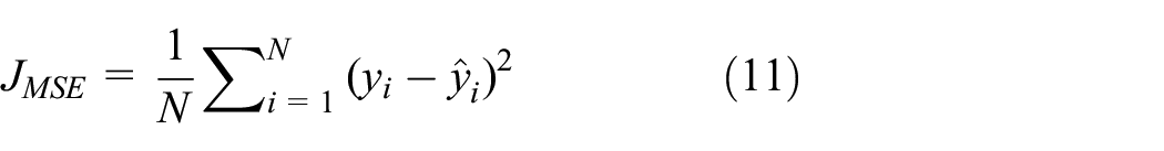
where N is the number of samples. $y_{i}$ and ${\hat{y}}_{i}$ are the original and predicted data.

Experiment and analysis

Dataset

The experimental data of acceleration sensors was generated from German side by using the software SIMPACK to simulate fault damages. SIMPACK is multibody dynamics (MBD) software used for mechanical system dynamics simulations and analyses.

The defects with wheel flats and radius differences are randomly generated and introduced into the simulation environment. A total of 64 sets of samples for wheel flats and 50 sets of samples with different radius are obtained for four wheel pairs. The resulting vibration signals are collected by the sensors with a sampling rate of 2000 Hz. Each case with a defect or non-defect situation for radius differences and wheel flats is separately stored in a folder. The folder name includes the information about the radius, the position of the worn wheel, and the height of a wheel flat (if available). Hence, the folder name indicates a defect or a non-defect situation. A label for a specific case will be assigned with value 0 (non-defect) or 1 (defect) for further training and validations.

The acceleration data for the eight wheels of a vehicle measured at the axle boxes are stored in eight files respectively. In each file, the acceleration of y- and z-directions are recorded over time. During the training and validation processes, the wavelet transform is applied to the acceleration data of the extracted 1024 time-series points. The results are used as input features (Table 2) fed to the deep learning network. Finally, the sampled data are divided into training and test sets at a ratio of 4:1. The data are saved as .tsv files.

Data preprocessing

The original z-axis data are preprocessed using the wavelet transform. The wavelet transform is specifically used for noise reduction in nonsmooth signals in this experiment, as shown in Figure 8. Then the transformed signals can be subsequently fed into the network for training.

Figure 8.

(a) Original fault signal. (b) Wavelet-transformed signal.

The wavelet basis function chosen for this experimental wavelet transform is db8, which belongs to the Daubechies wavelet family and is a discrete wavelet transform. The filter length is 16, which satisfies orthogonality, double orthogonality, and asymmetry.

Network structure

Fault diagnosis network structure

In this paper, three deep learning networks, ResNet, ResNet + SE, and ResNet + SE + SCL, are used for the fault diagnosis comparison. The hyperparameters associated with defining the neural network structure include the number of layers, the number of convolutional kernels, and the size of the convolutional kernels. The relevant hyperparameters are shown in Table 2.

Table 2.

Structurally relevant hyperparameters of ResNet, ResNet + SE, and ResNet + SE + SCL in the experiments.

Output size	ResNet	ResNet + SE	ResNet + SE + SCL encoder
1 $\times 1024 \times$ 2	input	input	input
64 $\times 1024 \times$ 2	conv(1,3)	conv(1,3)	conv(1,3)
64 $\times 1024 \times$ 2	RBU(64,3)	RBU + SE (64,3)	RBU + SE (64,3)
64 $\times 1024 \times$ 2	RBU(64,3)	RBU + SE (64,3)	RBU + SE (64,3)
128 $\times 512 \times$ 1	RBU(128,3,/2)	RBU + SE(128,3,/2)	RBU + SE (128,3,/2)
128 $\times 512 \times$ 1	RBU(128,3)	RBU + SE(128,3)	RBU + SE (128,3)
256 $\times 256 \times$ 1	RBU(256,3,/2)	RBU + SE (256,3,/2)	RBU + SE (256,3,/2)
256 $\times 256 \times$ 1	RBU(256,3)	RBU + SE (256,3)	RBU + SE (256,3)
512 $\times 128 \times$ 1	RBU(512,3,/2)	RBU + SE (512,3,/2)	RBU + SE (512,3,/2)
512 $\times 128 \times$ 1	RBU(512,3)	RBU + SE (512,3)	RBU + SE (512,3)
512	Pool	Pool	Pool
2	FC	FC

The learning rate is fixed to 0.0005. The batch size is chosen to be 128, and 50 epochs are trained. The SGD parameter optimizer is chosen.

The encoder network structure is similar to that of ResNet + SE. The difference is that supervised contrastive loss is used for the final pooled layer output to calculate the loss and optimize parameters. Then, the classifier, composed of a fully connected network layer, is trained on the basis of the optimized encoder parameters by using cross-entropy loss.

Fault degree prediction network structure

Because pretraining and finetuning method are used for the regression prediction task, the parameters are initialized with the trained ResNet + SE + SCL model parameters in the classification task and then fine-tuned by using mean squared difference loss. The batch size is set to 64, and 50 epochs are trained. The learning rate is initialized to 0.001; after 20 epochs, it is automatically reduced to 0.0001, and after another 20 epochs, it is reduced to 0.00001. The SGD parameter optimizer is chosen.

Experiments of fault diagnosis

The diagnosis of the presence of wheel radius difference and flats was performed using ResNet, ResNet + SE, and ResNet + SE + SCL.

Wheel radius difference

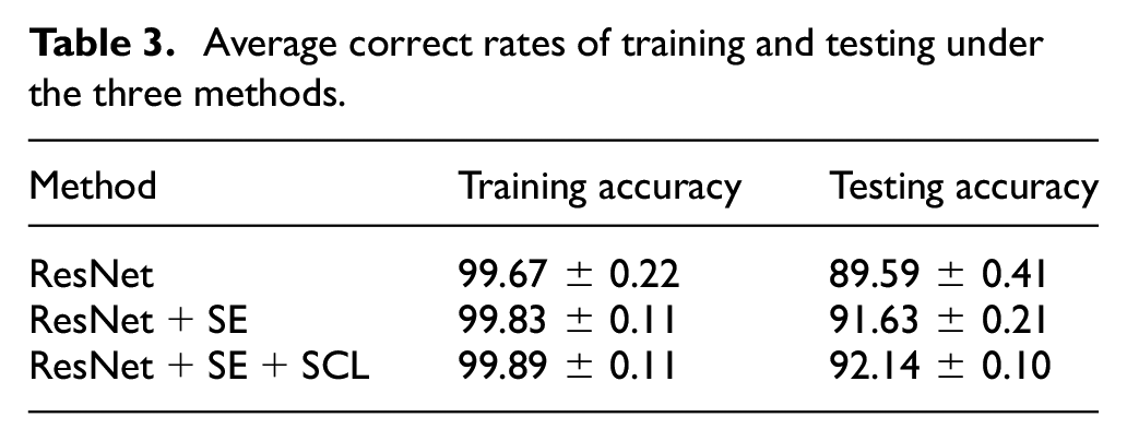
Table 3 shows the correct rates of ResNet, ResNet + SE, and ResNet + SE + SCL in determining the presence of wheel radius differences in wheel pairs. ResNet + SE and ResNet+SE+SCL improve by 2.04% and 2.55%, respectively, over the classical ResNet.

Table 3.

Average correct rates of training and testing under the three methods.

Method	Training accuracy	Testing accuracy
ResNet	99.67 ± 0.22	89.59 ± 0.41
ResNet+SE	99.83 ± 0.11	91.63 ± 0.21
ResNet+SE+SCL	99.89 ± 0.11	92.14 ± 0.10

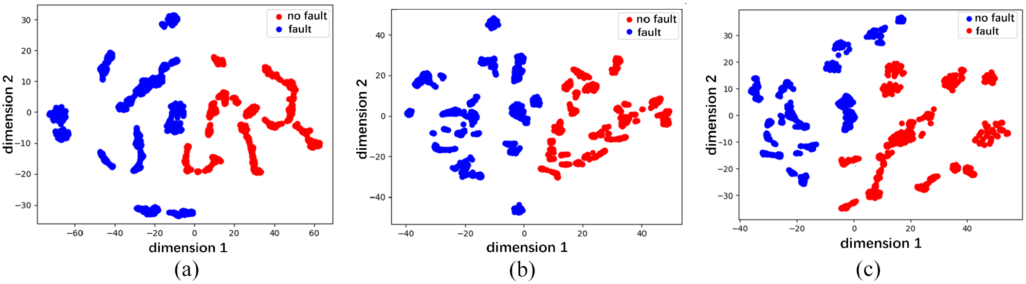
Then, nonlinear unsupervised dimensionality reduction methods, that is, T-distribution and random nearest neighbor embedding, are used for the visualization of high-level features of the pooling layer in two-dimensional (2D) space. Although visualization in 2D space is subject to some errors due to the loss of information during the dimensionality-reduction process, the purpose of 2D visualization is to provide an intuitive concept to determine whether these high-level features are distinguishable. As shown in Figure 9, a comparison of the classification effects of the three methods can be seen by the degree of mixing of the red and blue colors as follows: ResNet + SE+SCL> ResNet+SE > ResNet.

Figure 9.

2D visualization of the high-dimensional features of the wheel radius difference in the pool layer: (a) ResNet, (b) ResNet + SE, and (c) ResNet + SE + SCL.

The correctness rates of the training and test sets during training are shown in Figure 10. The correct rate of training for both ResNet + SE and ResNet in the figure is close to 100%, but in the test set, the correct rate of ResNet is lower than that of ResNet + SE. This is due to the introduction of the SE module and the soft threshold method as the systolic function in ResNet + SE, which improves the ability of the network to eliminate noise-related features. ResNet+SE+SCL makes it easier to distinguish the features of different fault classes, further improving the model’s noise resistance and fault diagnosis capabilities.

Figure 10.

Training and testing accuracy of the wheel radius difference: (a) ResNet, (b) ResNet + SE, and (c) ResNet + SE + SCL.

Wheel flats

As in the previous subsection, Table 4 shows the correct rates of determining the presence or absence of flats of the wheels for ResNet, ResNet + SE, and ResNet+SE+SCL. ResNet+ SE and ResNet + SE + SCL improve by 0.87% and 2.40%, respectively, over the classical ResNet. Figure 11 shows the two-dimensional visualization of the advanced features. Figure 12 shows the correct rates of the training set and the test set during the training process.

Table 4.

Average correct rates of training and testing under the three methods.

Method	Training accuracy	Testing accuracy
ResNet	99.83 ±v0.12	95.97 ± 0.22
ResNet + SE	99.92 ± 0.06	96.88 ± 0.14
ResNet + SE + SCL	99.97 ± 0.03	97.36 ± 0.09

Figure 11.

2D visualization of the high-dimensional features of the wheel flats in the pool layer: (a) ResNet, (b) ResNet + SE, and (c) ResNet + SE + SCL.

Figure 12.

Training and testing accuracy of the wheel flats: (a) ResNet, (b) ResNet + SE, and (c) ResNet + SE + SCL.

Similarly, ResNet + SE + SCL has a better classification capability. Therefore, the introduction of the SE module and SCL in ResNet can effectively improve the active learning capability of the model in identifying wheel flat features from wheel acceleration signals.

Experiments of fault degree prediction

To verify the accuracy of the regression model in predicting the fault degree, 60 sets of data were totally selected to test the regression model. The test results of wheel radius difference and wheel flat are shown in Figure 13. The horizontal coordinates in the figure indicate the samples, and the vertical coordinates indicate the wheel radius values. The blue line corresponds to the real value, while the orange line is the predicted value. The predicted value is compared with the actual value to clearly show the prediction effect of the regression model. It can be seen that the predicted value curves can fit well with the actual value curves for two wheel faults.

Figure 13.

Diagram of the predicted value of the regression task compared with the true value: (a) wheel radius difference and (b) wheel flat.

In this paper, the regression model was quantitatively evaluated for wheel radius difference and wheel flat using the mean squared error (MSE), mean absolute error (MAE), and R-squared⁴⁴ values. The results are shown in Table 5.

Table 5.

Results of regression model evaluation.

Evaluation Indices	MSE	MAE	R-squared
Wheel radius difference	4.35 $\times 10^{- 6}$	0.0016	0.76
Wheel flat	4.21 $\times 10^{- 6}$	0.0015	0.83

From the results of Table 5, it can be seen that the MSE and MAE values of the regression model are small and that the R-squared value is close to 1, indicating that the model has a good predictive ability for the fault degree. And the regression model has a better ability to predict the fault degree of wheel flat compared with wheel radius difference.

Interpretability about extracted features

In case of wheel defects, key features in defect-induced vibrations are amplified by structural resonances, not vehicle dynamics. The resonances of wheelset and track and their coupling are generally considered important below 500 Hz.⁴⁵

If the feature learning process aims to improve the SNR (signal-to-noise ratio) of features for better defect classification by suppressing or amplifying features according to their correlation with defects, the relationship between input and pooling layers can be considered as a transfer function of an adaptive filter in terms of signal processing. Therefore, it can be assumed that the feature learning method can obtain the proper transfer function in the form of amplifying these structural resonances and suppressing unnecessary features without prior knowledge. In order to verify whether the hypothesis is true, we carried out two steps:

Step1: Obtain features from input and pooling layers that contain the effects of the following three modes: (1) The second bending mode of the shaft @ 140 Hz, (2) The first umbrella mode of the wheel @ 230 Hz, (3) The first bending mode of the wheel @ 320 Hz.

Step2: Divide the pooling layer by the input layer after transforming features into the frequency domain and take the average value to obtain the averaged transfer function between both layers, as shown in Figures 14 and 15.

Figure 14.

Averaged transfer function of all defective cases for radius difference: (a) left wheel, and (b) right wheel.

Figure 15.

Averaged transfer function of all defective cases for wheel flats.

The magnitude of transfer functions at the three frequencies of 140, 230, and 320 Hz are amplified. At the same time, the low frequency range (below 50 Hz) related to vehicle dynamics is suppressed. Therefore, the hypothesis holds. It can be concluded that the feature learning process is well performed in this research.

Conclusion

Improving the feature-learning capabilities of deep learning models is an important task when applying these models to diagnose faults with noisy signals. The wheel radius difference and wheel flat fault diagnoses and prediction systems established in this paper use three network models: ResNet, ResNet + SE, and ResNet + SE + SCL. The SE module can learn global information relationships among the feature channels to enhance the ability of ResNet to extract useful information from the signal and reduce noise interference. Since SCL makes it easier to distinguish the features of different fault classes, it drives ResNet + SE + SCL to have a stronger learning ability and higher diagnostic performance than ResNet + SE. The improved network architectures are suitable not only for diagnosing faults but also for predicting the fault degrees by using pretraining and finetuning methods.

Footnotes

Handling Editor: Chenhui Liang

Author contributions

Yanxiang Chen: Conceptualization, methodology, investigation. Zuxing Zhao: Building the model, formal analysis, writing – original draft. Euiyoul Kim: Establishment of multibody system, simulation, calibration, and validation. Haiyang Liu: Validation, visualization. Juan Xu: Writing – review and editing. Hai Min: Supervision, software. Yong Cui: Conception of modeling and fault detection, project administration, writing – review and editing.

Declaration of conflicting interests

The author(s) declared no potential conflicts of interest with respect to the research, authorship, and/or publication of this article.

Funding

The author(s) disclosed receipt of the following financial support for the research, authorship, and/or publication of this article: This study was supported by the Anhui Provincial Key R&D Programmes – International S&T Cooperation (No. 202104b11020013), National Natural Science Foundation of China (No. 61972127), and Fundamental Research Funds for the Central Universities (No. PA2021KCPY0045).

ORCID iDs

Euiyoul Kim

Juan Xu

Yong Cui

References

Zhang

Chen

. Overview of rail fault diagnosis. System simulation technology and its application 2016; 18: 288–293.

Liu

Pan

Zuo

, et al. Progress of rail vehicle fault diagnosis research. J Mech Eng 2016; 52: 134–146.

Niu

Zhan

TY.

Research progress of rail vehicle fault diagnosis technology. China Sci Technol Overview 2018; 12: 54–55.

Shen

Wang

, et al. Train bearing fault diagnosis based on multiscale convolutional intra-class migration learning. J Transp Eng 2020; 20: 151–164.

Jiang

Zhao

, et al. An adaptive deep transfer learning method for bearing fault diagnosis. Measurement 2020; 151: 1–14.

Dong

Yang

WL.

Noise-resistant multi-core convolutional neural network-based bearing fault diagnosis method. J Beijing Univ Chem (Nat Sci Ed) 2020; 47: 100–106.

Liang

Yang

Wang

, et al. Research on the influence of train wheel diameter difference on traction system and corresponding protection measures. Railroad Cars 2018; 56: 33–37.

Liu

ZJ.

Hilbert-Huang transform-based fault diagnosis of train wheels out of round. J Meas Diagn 2016; 36: 734–739.

Lyu

Wang

Ling

, et al. Influence of wheel diameter difference on surface damage for heavy-haul locomotive wheels: measurements and simulations. Int J Fatigue 2020; 132: 1–10.

10.

Torabi

Mousavi

SGM

Younesian

A high accuracy imaging and measurement system for wheel diameter inspection of railroad vehicles. IEEE Trans Ind Electron 2018; 65: 8239–8249.

11.

Sui

Wang

Ling

, et al. Effect of wheel diameter difference on tread wear of freight wagons. Eng Fail Anal 2021; 127: 1–16.

12.

Zhang

Ren

, et al. Deep residual learning for image recognition. In: 2016 IEEE conference on computer vision and pattern recognition, Las Vegas, NV, USA, 27–30 June 2016, pp.770–778.

13.

Shen

Albanie

, et al. Squeeze-and-excitation networks. IEEE Trans Pattern Anal Mach Intell 2020; 42: 2011–2023.

14.

Chen

Kornblith

Norouzi

, et al. A simple framework for contrastive learning of visual representations. In: International conference on machine learning, Vienna, Austria, 13–18 July 2020, pp.1597–1607.

15.

Fan

, et al. Momentum contrast for unsupervised visual representation learning. In: Proceedings of the IEEE/CVF conference on computer vision and pattern recognition (CVPR), Seattle, USA, 16–18 June 2020, pp.9729–9738.

16.

Khosla

Teterwak

Wang

, et al. Supervised contrastive learning. In: 34th conference on neural information processing systems (NeurIPS 2020), Vancouver, Canada, 6–13 December 2020, pp.1–23.

17.

Corni

Symonds

Wood

RJK

, et al. 2015. Real-time on-board condition monitoring of train axle bearings. In: The Stephenson Conference, IMechE, London, UK, 2022 April 2015, pp.1–14.

18.

Dalpiaz

Rivola

Rubini

Effectiveness and sensitivity of vibration processing techniques for local fault detection in gears. Mech Syst Signal Process 2000; 14: 387–412.

19.

Baillie

Mathew

A comparison of autoregressive modeling techniques for fault diagnosis of rolling element bearings. Mech Syst Signal Process 1996; 10: 1–17.

20.

Xiukun

Ying

Limin

, et al. Fault detection of rail vehicle suspension system based on CPCA. In: Conference on control and fault-tolerant systems (SysTol), Nice, France, 9–11 October 2013.

21.

Mei

Ding

XJ.

Condition monitoring of rail vehicle suspensions based on changes in system dynamic interactions. Veh Syst Dyn 2009; 47: 1167–1181.

22.

Zheng

Song

, et al. A fault diagnosis method of bogie axle box bearing based on spectrum whitening demodulation. Sensors 2020; 20: 7155.

23.

Nowakowski

Komorski

Szymański

, et al. Wheel-flat detection on trams using envelope analysis with Hilbert transform. Lat Am J Solids Struct 2019; 16: 1–16.

24.

Baasch

Heusel

Roth

, et al. Train wheel condition monitoring via cepstral analysis of axle box accelerations. Appl Sci 2021; 11: 1432.

25.

Liang

Iwnicki

Zhao

, et al. Railway wheel-flat and rail surface defect modelling and analysis by time–frequency techniques. Veh Syst Dyn 2013; 51: 1403–1421.

26.

Krummenacher

Ong

Koller

, et al. Wheel defect detection with machine learning. IEEE Trans Intell Transp Syst 2018; 19: 1176–1187.

27.

Jiang

Lin

Fault diagnosis of wheel flat using empirical mode decomposition-Hilbert envelope spectrum. Math Probl Eng 2018; 2018: 1–16.

28.

Sun

Wang

Zhang

. Fault diagnosis method of autonomous underwater vehicle based on deep learning. In: IOP conference series: material science and engineering, Paris, France, 23–25 July 2019, pp.1–6.

29.

Zhao

Tang

Deng

, et al. Multiple wavelet regularized deep residual networks for fault diagnosis. Measurement 2020; 152: 1–11.

30.

Chu

Han

Deep residual learning with demodulated time-frequency features for fault diagnosis of planetary gearbox under nonstationary running conditions. Mech Syst Signal Process 2019; 127: 190–201.

31.

Zhao

Zhong

, et al. Deep residual shrinkage networks for fault diagnosis. IEEE Trans Ind Inform 2020; 16: 4681–4690.

32.

Luo

Cole

, et al. An overview: modern techniques for railway vehicle on-board health monitoring systems. Veh Syst Dyn 2017; 55: 1045–1070.

33.

Jardine

AKS

Lin

Banjevic

. A review on machinery diagnostics and prognostics implementing condition-based maintenance. Mech Syst Signal Process 2006; 20: 1483–1510.

34.

Cao

Sun

Xing

. Safety region estimation and fault diagnosis of wheels based on LSSVM and PNN. In: AIP conference proceedings, Santiago, Chile, 2017, vol. 1820.

35.

Wang

Liu

Bao

. Deep learning neural network for power system fault diagnosis. In: Proceedings of the 35th Chinese control conference, Chengdu, China, 27–29 July, 2016, pp.27–29.

36.

Zhang

Sanuncn

. 2018. Generalized cross entropy loss for training deep neural networks with noisy labels. In: 32nd conference on neural information processing systems (NeurIPS 2018), Montreal, QC, Canada, 2018, pp.8778–8788.

37.

Elasayed

Krishnan

Mobahi

, et al. Large margin deep networks for classification. In: 32nd conference on neural information processing systems (NeurIPS 2018), Montreal, QC, Canada, 2018, pp.842–852.

38.

Oord

AVD

Vinyals

. Representation learning with contrastive predictive coding. arXiv preprint arXiv:1807.03748, 2018.

39.

enaff

OJH

Srinivas

Fauw

, et al. Data-efficient image recognition with contrastive predictive coding. In: International conference on machine learning, Vienna, Austria, 13–18 July 2020, pp.4182–4192.

40.

Zhou

Xiong

, et al. Prototypical contrastive learning of unsupervised representations. arXiv preprint arXiv:2005.04966, 2020.

41.

Kalantidis

Sariyildiz

Pion

, et al. Hard negative mixing for contrastive learning. arXiv preprint arXiv:2010.01028, 2020.

42.

Tian

Sun

Poole

, et al. What makes for good views for contrastive learning. In: 34th conference on neural information processing systems (NeurIPS 2020), Online, 6–12 December 2020, pp.1–24.

43.

Guo

Xia

Luo

, et al. Remote sensing image scene classification based on supervised contrastive learning. J Photonics 2021; 50: 87–98.

44.

CFI. What is R-Squared, https://corporatefinanceinstitute.com/resources/knowledge/other/r-squared/ (2020, accessed 6 December 2021).

45.

Rakheja

Ahmed

, et al. Influence of a flexible wheelset on the dynamic responses of a high-speed railway car due to a wheel flat. Proc IMechE, Part F: J Rail and Rapid Transit 2018; 232: 1033–1048.

Wheel fault diagnosis model based on multichannel attention and supervised contrastive learning

Abstract

Keywords

Introduction

Related work

Fault diagnosis and prediction system of wheel radius difference and wheel flat

Mechanical description of wheel fault

Fault diagnosis and prediction system

ResNet + SE

ResNet + SE + SCL

Regression model

Experiment and analysis

Dataset

Data preprocessing

Network structure

Fault diagnosis network structure

Fault degree prediction network structure

Experiments of fault diagnosis

Wheel radius difference

Wheel flats

Experiments of fault degree prediction

Interpretability about extracted features

Conclusion

Footnotes

Author contributions

Declaration of conflicting interests

Funding

ORCID iDs

References