Sage Journals: Discover world-class research

Abstract

RPThe wheel condition monitoring when the train in operation is significant task to prevent the occurrence of unexpected event. In this study, the piezoelectric sensors were installed on the railway track to collect the dynamic voltage-and-strain signals when the train wheels pressed them. These one-dimensional time series signals were transformed to the two-dimensional Recurrence Plots (RP) images as an input data sets for two deep learning models, Xception and EfficientNet-B7. The binary classification, Normal or Faulty as the diagnostical output to indicate the health state of the train wheels in that time. Five metrics were selected to evaluate the performance of two models, namely Accuracy, Precision, Recall, Miss Rate, and AUC. The results show that both models perform the high accuracy of 91.1% to the wheel condition classification. Furthermore, EfficientNet-B7 shows better performance in Recall, Miss-rate, and AUC metrics than those of Xception to express the premium ability in defective wheel identification, which is crucial for this application. Therefore, the efficientNet-B7 is selected as a favorable machine learning classifier for the fault diagnosis of rolling stock wheels. It is significant contribution to train wheel condition monitoring and health management since it provides the effective diagnostic information for maintenance decision to decrease the occurrence of unexpected event.

Keywords

Recurrence plot convolutional neural networks condition monitoring train wheel fault diagnosis

Introduction

A wheel-axle set is a critical assembly for a railroad car and it represents the complex dynamic behavior when the train is in high-speed motion on the railway. The wheel defects such as out of roundness, corrugation, flat, roughness, discrete defects, spalling, shelling, and so on affect their smooth revolutions that subsequently induce damage in the rails and wheel itself due to high impact forces in the wheel–rail interface. Traditionally, cracks and other abnormalities on the wheel could be found by professionals in their regular inspection. However, it can be limited by the conditions of human work corresponding with physical, mental, and even social health. In recent years, various sensors are installed on the rail or the wheelset to measure the signals of vibration, strain, and acoustic that indicate the operating states (healthy or abnormal) of train, called condition monitoring, CM.^1–4 For instance, Sun et al.⁵ present a detection methodology based on the angle domain synchronous averaging technique (ADSAT) to monitor the conditions of axle-box bearings by the vibration signals. Gao et al.⁶ show a new optical position sensor mounted on rails to measure the wheel-rail impact force by detecting the displacement of the collimated laser spot. Stratman et al.⁷ propose wheel impact load detectors (WILDs) for trains while in service to collect real-time data regarding with structural failure of railroad wheels. These studies show that the approach is able to identify the potential defect instantaneously according to the diagnosis or prognostics of collected data using the appropriate model. Once the abnormal situation is detected, the maintenance work will be performed to prevent the occurrence of failure of the monitoring asset. How to keep wheels in an adequate condition and to detect defect effectively have become the advanced research topics in predictive maintenance of railway system in recent years.^8–10

Machine learning (ML) has been one of the most attractive research topics in engineering over the last several decades. Recently Deep Learning (DL) has been developing to extract higher-level features compared to only one hidden layer of traditional Artificial Neural Networks (ANN). For railway engineering applications, several studies indicate that machine learning can be used as the alternative model compared to the classical computational ones for the calculation of the wheel-rail contact location or the estimation of the wheel-rail contact loadings.¹¹ Furthermore, it can be found in the scientific articles how artificial intelligence has captured more attention to the researchers for the area of railway engineering in recent years^12–15 Besides, cloud computing with 5G communication, Internet of Things (IoT), and ML technologies has also gained huge popularity for various applications. In the modern cloud-based railway control system, it is able to rapidly collect and process data associated with axle loads, track geometry, velocity records, thermal data, and so on. Then a lot computing was performed to fast deliver the services regarding with axle fault diagnosis, condition monitoring of assets to instantaneously provide the best reference for decision making at minimal cost.^16–20 Although the signal could be proceeded to reproduce the characteristics of the defect pattern in actual application of CM in railway wheel, not all of the defects represent obvious characteristics in the signal especially in the early stage of fault developing. As a result, the difficulty exists with respect to the feature identification of small defects using machine learning models.

Recurrent Plot (RP), a visualization technology for nonlinear data regression analysis, was proposed by Eckmann et al.²¹ in 1987 to analyze the recursive characteristics of time series in phase space. It improves analytical performance of the time series data, especially in non-stationary with high noise situation including small defects or features. Taghizadegan et al.²² proposed a dynamic model based on sleep graph signals regarding with electroencephalography (EEG), electrocardiogram (ECG) and respiratory ones. They established RP images from these signals, and then imported them into the two Convolutional Neural Networks (CNN) named ResNet-18 and ShuffleNet. Finally, the best model was selected by evaluating the performance metrics regarding with the model accuracy, sensitivity, specificity, precision, receiver operating characteristic (ROC), and area under the curve (AUC). Li et al.²³ presented a multi-label CNN to extract the various damage feature in RP, and to identify the structural damage by multi-classification. The results show that the CNN has high operational efficiency for different damage location extracted from RPs to identify various vibration modes of the structure. More studies^24–28 applied RP to generate effective images and input the deep learning CNN models to classify targets, and they have confirmed that using RP with deep learning, especially CNN-based model, can effectively extract more features in various domain problems and improve the accuracy of prediction. To the best of our knowledge, there is rarely research to analyze the rotating wheel defects of railway based on the method of RP and CNN- model.

In this study, the piezoelectric sensors were installed on the railway track to collect the dynamic voltage-and-strain signals when the wheels of the train pressed the measurement location. These one-dimensional time series signals were transformed to the two-dimensional RP images as an input data sets for two deep learning models, named Xception and EfficientNet-B7. The binary classification, Normal or Faulty as the output of the model to indicate the health state of the train wheels. The normal condition wheels and wheels with defects have been known a priori in the training data. The metrics of accuracy, precision, sensitivity, miss rate, and AUC were calculated to assess the performance for each model. The diagnostic result show that both models represent their high accuracies of prediction, and the EfficientNet-B7 model shows higher recall (sensitivity) number and lower miss rate one to express the premium ability in defective wheel identification, which is crucial for this application. It is significant contribution to train wheel condition monitoring and health management using a novel combined RP-CNNs methodology developed in this study since it provides the effective diagnostic information for maintenance decision to decrease the occurrence of unexpected event.

Methods

Recurrence plot (RP)

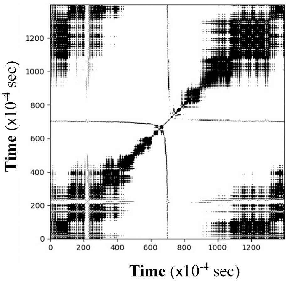
Recurrence plot is a visualization technique for nonlinear data regression analysis which is focused on the dynamic path of a time series data in the state space, shown as Figure 1. A time delay method is usually used to obtain all of the possible states. RP can improve the steady-state reduction phenomenon when the length of time series increases, especially in the type of non-stationary with high-noise signals.^29–30 For a one-dimensional time series data with parameter x and length n is {x_i, i = 1, 2, 3, …, n}. Reconstruct the phase state trajectory of the system of x, and obtain the system state delay vector u_j in the high-dimensional phase space as follows:

u_{j} = (x_{j}, x_{j + τ}, \dots, x_{j + (m - 1) τ}), j = 1, 2, \dots, N

(1)

where x_j is state quantity of the x signal in the m-dimensional phase space; m is embedding dimension; τ is time delay (Embedding Lag); $N = n - (m - 1) \times τ$ is the number of the system state. Appropriate τ and m are able to generate a fully expanded geometric structure of the phase space with parameter x, and thus can accurately describe the dynamic trajectories of all possible states of the system.

Figure 1.

Recurrence plot.

The recurrence phenomenon is one of the essential laws of the state evolution of a complex dynamic system (the another one is chaos). Periodic recursion occurs in the state trajectory of the system. The RP is a tool to visualize the recurrence of the state by drawing a two-dimensional plane regarding with a symmetric R matrix of size $[N - (m - 1) \times τ] \times [N - (m - 1) \times τ]$ . The value R of the j^th row and the k^th column of the RP can be expressed as follows:

R (j, k) = {\begin{matrix} 1 (d (u_{j}, u_{k}) \leq r) \\ 0 (d (u_{j}, u_{k}) > r) \end{matrix}

(2)

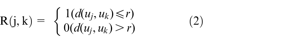
where d(•) is the Euclid distance between u_j and u_k; r is the preset threshold distance. If the distance between u_j and u_k is less than or equal to r, it means that the state of the system at time j and time k is very similar. As the result, the trajectory represents that the state of the system appears recursive. Then the (j, k) position is represented by a black dot in the RP. On the contrary, if the distance between u_j and u_k is greater than r, it means that the two states are far apart. The value of R is set to 0 and the (j, k) positions are indicated by a white dot. In terms of feature display of the RP, if the signal is random, the distribution of points is uniform; if it is a periodic signal, such as a sine wave, there will be obvious and fixed regular distribution. The horizontal or vertical black lines of the RP represent the data in a period of time, and the state of the system has not changed significantly, while the line segments parallel to the main diagonal represent the trajectories of the system in the phase space in different time periods.

Xception

Xception was developed by the Chollet (Google)³¹ as the successor of InceptionV3 where it presented a novel deep convolutional neural network structure that refers deepwise separable convolution and a pointwise convolution³² to take advantages of lower computational complexity and higher classification performance compared to the series of Inception models.

The model consists of 36 convolutional layers. The linear residual connections were designed into the intermediate blocks to solve the vanishing gradient problem. Figure 2 shows the primary module of Xception inspired by the Inception where it was called extreme version of Inception.³¹ It can be seen that 1 × 1 convolution was applied to mapping multi-channel correlations followed by several 3 × 3 convolution operations (one for each channel) to separately aligning the spatial correlations, and finally concatenating was performed to combine these 3 × 3 columns into a single vector-valued one. Compared to the Inceptions V3, the Xception represents more efficient use of model parameters during the whole calculating process to improve the model performance for the classification task with large-scale images.

Figure 2.

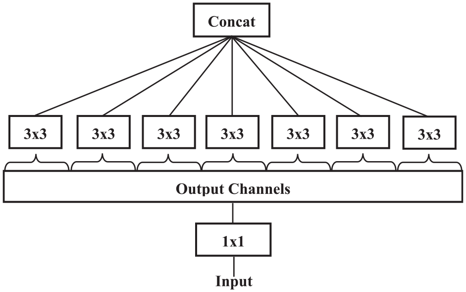
Schematic representation of Xception.

EfficientNets

EfficientNet was developed by Tan and Le in 2020³³ to improve the efficiency of computation since the large CNN structure is generally limited by the hardware memory when training the model. Compared to the Xception of using model parameters efficiently to increase the model performance, the EfficientNet is tend to scaling up the model by considering network depth, width, and resolution simultaneously. Tan and Le introduced a novel compound scaling method by using a compound coefficient φ to uniformly scales network width, depth, and resolution during the process of training model. For instance, if the size of an input image is large, the network depth and width should be enlarged to increase the receptive field and catch the fine-grained patterns on a high-resolution image. The principles of the model and compound coefficient φ³³ are given in equation (3)

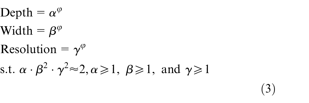
\begin{matrix} Depth = α^{φ} \\ Width = β^{φ} \\ Resolution = γ^{φ} \\ s . t . α \cdot β^{2} \cdot γ^{2} \approx 2, α \geq 1, β \geq 1, and γ \geq 1 \end{matrix}

(3)

where α, β, γ are constants which can be determined by a grid search; φ depends on the hardware resources to control the scaling process. For example, if there is 2^N times more computational resources, then the network depth, width, and image size can be simply increased by α^N, β^N, and γ^N respectively. Figure 3 presents a schematic layout of EfficientNet-B7 used in this study, which has 66 million parameters and takes a 600 × 600 image as input. Three layers, global average pooling2D, dropout, and dense were applied, and they were all activated by a RELU function. There are two classifications, normal or faulty as an output layer. A softmax activation function were used to be a classifier.

Figure 3.

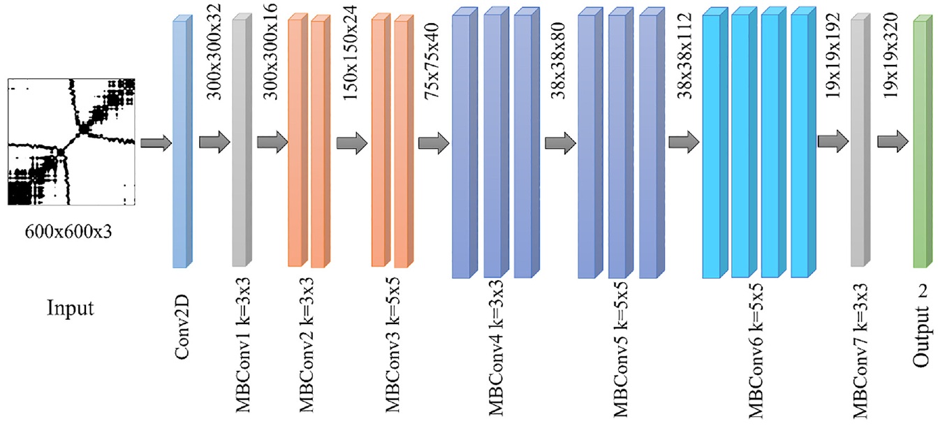
Schematic representation of EfficientNet-B7.

The strain measurement and data processing

Figure 4 presents the whole operational process for fault diagnosis of railway wheels. Part I indicates the strain measurement and signal processing. Part II specifies data featuring process associated with graphing voltage-strain diagrams, sampling vulnerable fragment, and transforming to recurrence plots. Part III states the process of modeling and evaluating to select optimal one for the application of railway wheel diagnosis. The details of several critical sections will be illustrated as below:

Figure 4.

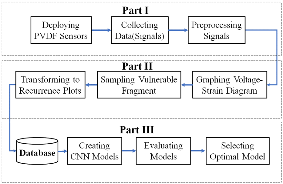
The whole process of operation for fault diagnosis of railway wheels.

The PVDF sensors were deployed to the train transport system. Figure 5 shows the setup positions of the PVDF piezoelectric sensors³⁴ on a rail track where located at the vicinity of a local railway station with relatively dense traffic. Several encapsulated sensor arrays were mounted to the side and bottom of the rail in between two sleepers. A DAQ equipment was used to directly measure the response of sensors regarding with dynamic voltage/strain signals while the train passed across them. The signal was carried out to diagnose defects in train wheel surfaces and to estimate the timing of predictive maintenance.

Figure 5.

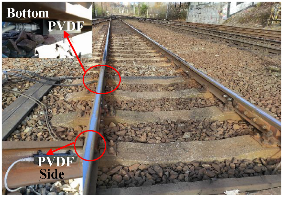
The setup locations of the PVDF piezoelectric sensors on a rail track.

Figure 6 depicts the voltage and strain response signals by collecting data from the PVDF strain sensor module. The greatest value of strain occurs at the bottom of concave strain curve while the center of the train wheel passed across the measurement point of the sensor. At the same time, the voltage deeply dropped and then increase again. However, the signal of voltage looks better than that of strain for classification using machine learning technique since the former one represents obvious fluctuations especially in a nearby area of the lowest point (strain curve), which means that more features regarding with small faults on the train could be extracted by the deep learning model to increase the prediction accuracy. To sampling vulnerable fragment, 1400 measurement points located both sides of the lowest point for the voltage curve were selected as an input data, and then the 1-D signal was transformed into 2-D images. In addition, the image enhancement technique was applied to increase the quality of these images for performance improvement of these two models.

Figure 6.

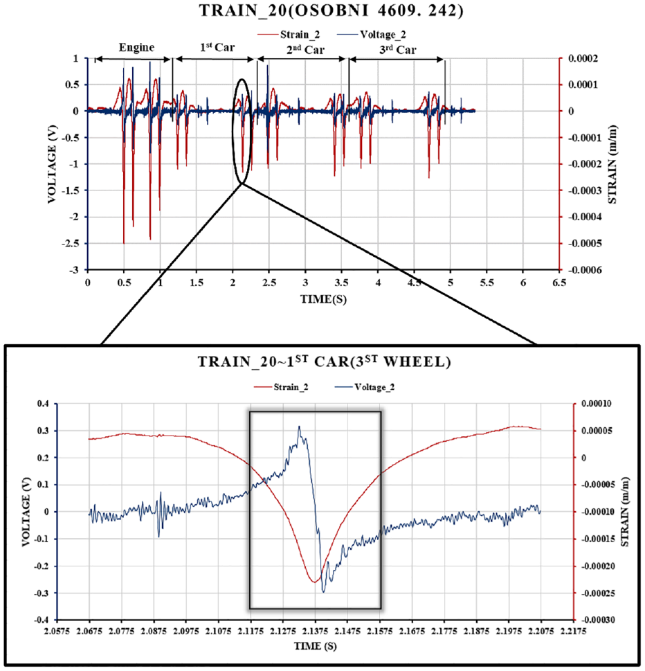
The voltage and strain response signals by the PVDF stain sensor module.

Figure 7 presents the Black-and-White Recurrence Plot transformed from the voltage curve of fourth wheel of second car of Train_20 (Figure 5). The size of each RP image is 500 × 500 pixels for the Xception and 600 × 600 pixels for the EfficientNet-B7. The total 334 RP images have been successfully transformed as the input dataset. Two classes, 0 for normal and 1 for faulty were assigned to diagnose whether the train wheel was in health state or not. The ratio of a training set and validation one is 7:3 for this small dimensional dataset.

Figure 7.

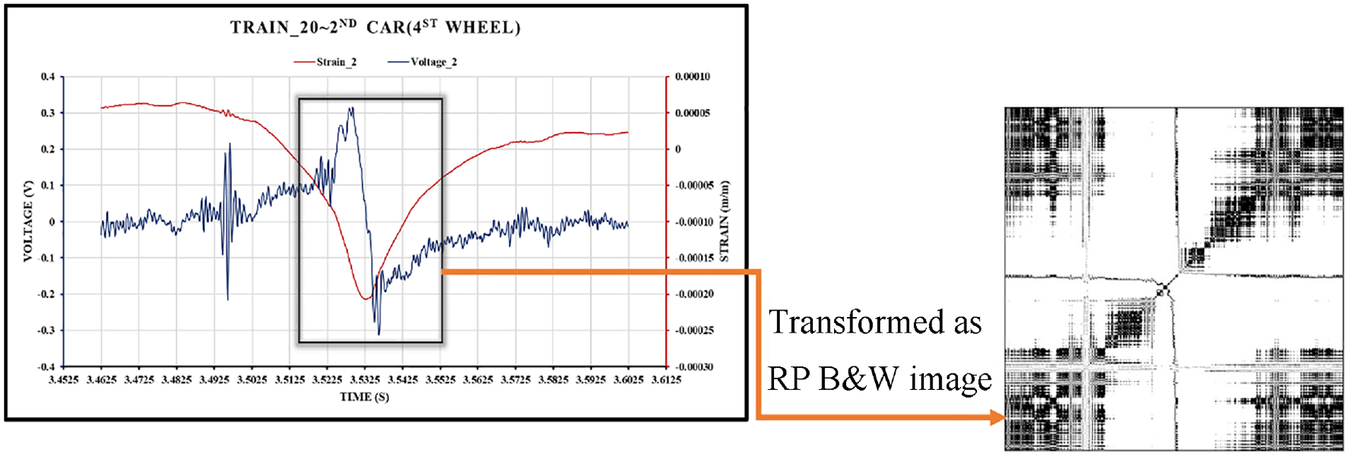
The RP transformation from the voltage curve of fourth wheel of second car of Train_20.

Results and discussion

Figure 8 shows the model training, testing, and evaluation process. There are 233 and 101 images were as inputs for training and testing the model respectively.

Figure 8.

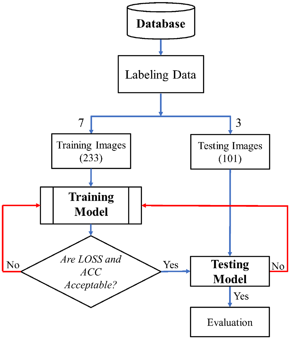
The process of model training, testing, and evaluation.

Model training

Figure 9 shows the loss (left) and accuracy (right) curves per epoch of the training and validation data (both in the training data set) to the Xception model. It can be seen that the gap between train and validation loss is small and that the curves in the validation and train data are similar resulting the conformity in both training and validation data. Moreover, the loss function decreases with the increase of the number of iterations, and the accuracy (ACC) increases with the increase of the number of epochs as well. As the results, the model provides a low validation loss of 0.121 and a high validation accuracy of 95.8% at the last epoch of 800.

Figure 9.

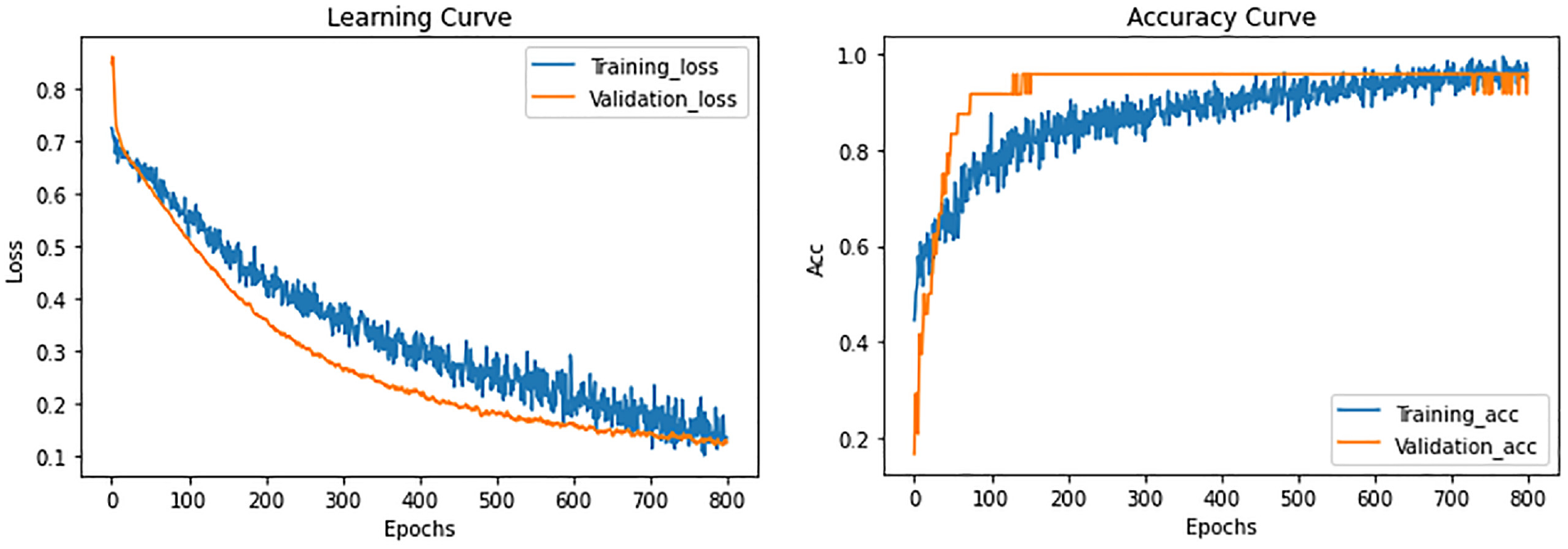
The loss (left) and accuracy (right) curves per Epoch of the training and validation sets obtained using Xception.

Figure 10 presents the loss (left) and accuracy (right) curves per epoch of the training and validation data (both in the training data set) to the EfficientNet-B7 model. It is seen that the gap between train and validation loss of EffecientNet-B7 is greater than that of Xception though, the loss function decreases with the increase of the number of iterations and the accuracy (ACC) increases with the increase of the number of epochs. For the same last epoch of 800 with Xception, the Efficient-Net-B7 provides a reasonable validation loss of 0.270 and accuracy of 87.5%.

Figure 10.

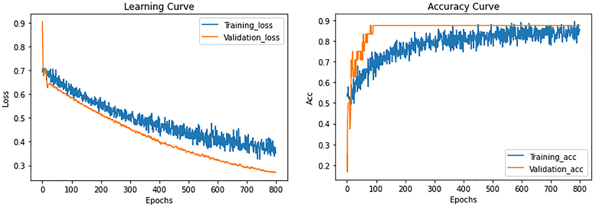
The loss (left) and accuracy (right) curves per Epoch of the training and validation sets obtained using EfficientNet-B7.

Model testing

Figure 11 shows confusion matrix obtained using the test data set for these two models. There are 101 images were used to testing the deep learning models unknown a priori. From the confusion matrix, each cell represents the number of images of a given class (true label) classified into the class indicated by the column (predicted label). A perfect classifier will only have total 101 images in the matrix diagonal (no two types of errors). It is observed that the Xception model can identify 28 images correctly in the “Normal” class, but 3 images were labeled as “Faulty” ones. For EfficientNet-B7 model, there are 20 images can be correctly classified in the “Normal” class but 11 images were labeled as “Faulty” ones. The Xception model reveals the better performance to label the normal train wheel images resulting the lower type I errors. However, it is even more crucial in the situation that “Faulty” train wheel was identified to be “Normal” train one (type II error) because the failure of the wheel could occur in the operation state to lead the series accident for public transportation, and it only increase the maintenance cost for the type I error. As seen the Figure 9 again, Xception can identify 64 images correctly in the “Faulty” class, 6 images were labeled as “Normal” ones. For the EfficientNet-B7 model, there are 67 images can be correctly classified in the “Faulty” class but only 3 images were labeled as “Normal” ones. It is more significant that the EfficiencyNet-B7 model presents the better performance in classified the faulty train wheel images resulting the lower type II errors.

Figure 11.

The confusion matrix obtained using the test data for two models: (a) Xception and (b) EfficientNet-B7.

Table 1 exhibits five metrics to estimate the performance of Xception and EfficientNet-B7 models, namely Accuracy, Precision, Recall, Miss Rate, and AUC. The accuracy presents the general metric which is the percentage of correctly predicted image classes (including the TP and TN) to the total number of images; precision is the fraction of images correctly labeled as the positive class (true faulty wheel, TP) divided by the total number of images labeled as the positive class (TP plus FP); The recall is the proportion of actual positives correctly identified by the models that is the number of true positives (TP) divided by the number of true positives plus the number of false negatives (TP plus FN). Recall is expected to have nearest number to one which represents the highest sensitivity or lowest miss rate (1-sensitivity) for the model to identify all of the true faulty wheels. Both of them are the most important metrics for the application. AUC, the area under receiver operating characteristics, indicates how well the model can distinguish between classes whose range is from 0 to 100%. If a model having an AUC scores close to 100%, it is considered the best model.

Table 1.

The performance valuation of two models.

DL ModelMetrics	Xception	EfficientNet-B7
Accuracy (%)	91.1	91.1
Precision (%)	95.5	91.8
Recall (%) (sensitivity)	91.5	95.7
Miss rate (%) (1-sensitivity)	8.5	43
AUC (%)	76.0	91.0

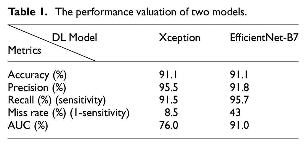
As seen in the Table 1, the accuracies for these two models are the same of 91.1% to represent that both models have the high absolute percentage of images correctly classified. The precisions are 95.5 and 91.8% for Xception and EfficientNet-B7 respectively. Although the EfficientNwt-B7 reveals a higher number of 67 in TP, it also gives a higher number of 6 in FP (type I error), and thus represents a worse performance in precision. However, efficientNet-B7 presents higher recall (sensitivity) number of 95.7% and lower miss rate (1-sensitivity) number of 4.3% than those numbers of 91.5 and 8.5% respectively for Xception. It indicates that the actual defective wheel is predicted by the EfficientNet-B7 model to have a lower False Negative Rate (type II model) than that of the Xception. The AUC of the EfficientNet-B7 and the Xception are 91.0 and 76.0% respectively to demonstrate that the EfficentNet-B7 has a much lower probability than that of Xception to distinguish between wheel with normal class and wheel with faulty class. In summary, both models perform the high accuracy of 91.1% to the wheel condition classification. Furthermore, EfficientNet-B7 shows better performance in Recall, Miss-rate, and AUC metrics than those of Xception to express the premium ability in defective wheel identification, which is crucial for this application. Therefore, the efficientNet-B7 is selected as a favorable machine learning classifier for the fault diagnosis of rolling stock wheels.

Conclusions

In this study, two deep learning model, Xception and EfficientNet-B7 were applied to classify the health condition (Normal or Faulty) for the train wheels in operation. The 1D strain-and-voltage signals measured by the PVDF sensors were transformed to the 2D recurrence plots as the input images for the deep learning models. the accuracies for these two models are the same of 91.1% to represent that both models have the high absolute percentage of images correctly classified. The Xception model performs the better performance in precision than that of the EfficientNet-B7 (95.5 vs 91.8%). However, the EfficientNet-B7 model presents higher recall (sensitivity) number of 95.7% and lower miss rate (1-sensitivity) number of 4.3% than those numbers of 91.5 and 8.5% respectively for the Xception one to express the premium ability in defective wheel identification, which is crucial for this application. Therefore, the efficientNet-B7 is selected as a favorable machine learning classifier for the fault diagnosis of rolling stock wheels. It is significant contribution to train wheel condition monitoring and health management since it provides the effective diagnostic information for maintenance decision to decrease the occurrence of unexpected event.

In the future, the model performance may be improved using more datasets to increase the extraction rate of the features regarding with various defect patterns. In addition, more sophisticated feature extraction techniques such as U-Net, and You-Only-Look-Once (YOLO) could be applied as preprocessor to segment the interesting features in the images to increase the performance of classification.

Footnotes

Acknowledgements

We would additionally like to thank the Drazni revize ltd., Brno University of Technology and Alis, ltd., Czech Rep., for providing the measurement data and some professional discussion in this international (Czech Rep.-Taiwan) cooperation project.

Declaration of conflicting interests

The author(s) declared no potential conflicts of interest with respect to the research, authorship, and/or publication of this article.

Funding

The author(s) disclosed receipt of the following financial support for the research, authorship, and/or publication of this article: The authors would like to thank Ministry of Science and Technology of Taiwan for the financial support that made this research work possible under grant no.109-2923-E-194-MY3.

ORCID iD

Kuan-Jung Chung

References

Schwendemann

Amjad

Sikora

. A survey of machine-learning techniques for condition monitoring and predictive maintenance of bearings in grinding machines. Comput Ind 2021; 125: 103380.

Theissler

Pérez-Velázquez

Kettelgerdes

, et al. Predictive maintenance enabled by machine learning: use cases and challenges in the automotive industry. Reliab Eng Syst Saf 2021; 215: 107864.

Lee

Singh

, et al. Intelligent maintenance systems and predictive manufacturing. J Manuf Sci Eng 2020; 142: 110805.

Ghofrani

Hea

Goverde

, et al. Recent applications of big data analytics in railway transportation systems: a survey. Transp Res Part C 2018; 90: 226–246.

Sun

Chen

Kemp

, et al. An on-board detection framework for polygon wear of railway wheel based on vibration acceleration of axle-box. Mech Syst Signal Process 2021; 153: 107540.

Gao

Feng

, et al. In-service detection and quantification of railway wheel flat by the reflective optical position sensor. Sensors 2020; 20: 4969.

Stratman

Liu

Mahadevan

. Structural health monitoring of railroad wheels using wheel impact load detectors. J Fail Anal Prev 2007; 7: 218–225.

Alemi

Corman

Lodewijks

. Condition monitoring approaches for the detection of railway wheel defects. Proc IMechE, Part F: J Rail and Rapid Transit 2017; 231: 961–981.

Tao

Wen

Jin

, et al. Polygonisation of railway wheels: a critical review. Rail Eng Sci 2020; 28(4): 317–345.

10.

Sedghi

Kauppila

Bergquist

, et al. A taxonomy of railway track maintenance planning and scheduling: a review and research trends. Reliab Eng Syst Saf 2021; 215: 107827.

11.

Falomi

Malvezzi

Meli

, et al. Determination of wheel-rail contact points: comparison between classical and neural network based procedures. Meccanica 2009; 44: 661–686.

12.

Urda

Aceituno

Muñoz

, et al. Artificial neural networks applied to the measurement of lateral wheel-rail contact force: a comparison with a harmonic cancellation method. Mech Mach Theory 2020; 153: 1–17.

13.

Mohammadi

Ghofrani

, et al. Exploring the impact of foot-by-foot track geometry on the occurrence of rail defects. Transp Res Part C 2019; 102: 153–172.

14.

Pires

Mendes

Santos

, et al. Indirect identification of wheel rail contact forces of an instrumented heavy haul railway vehicle using machine learning. Mech Syst Signal Process 2021; 160: 107806.

15.

Sysyn

Gerber

Nabochenko

, et al. Prediction of rail contact fatigue on crossings using image processing and machine learning methods. Urban Rail Transit 2019; 5: 123–132.

16.

Singh

Elmi

Meriga

, et al. Internet of things for sustainable railway transportation: past, present, and future. Clean Logist Supply Chain 2022; 4: 100065.

17.

Zhou

Dumss

Nowak

, et al. A conceptual model-based digital twin platform for holistic large-scale railway infrastructure systems. Procedia CIRP 2022; 109: 362–367.

18.

Milić

Miladinović

Rakić

. A wayside hotbox system with fuzzy and fault detection algorithms in IIoT environment. Control Eng Pract 2020; 104: 104624.

19.

Cai

Wang

, et al. Deep reinforcement learning framework-based flow rate rejection control of soft magnetic miniature robots. IEEE Trans Cybern. Epub ahead of print 7 September 2022. DOI: 10.1109/TCYB.2022.3199213.

20.

Cai

Wang

, et al. Autonomous manipulation of an underwater vehicle-manipulator system by a composite control scheme with disturbance estimation. IEEE Trans Autom Sci Eng. Epub ahead of print 12 January 2023. DOI: 10.1109/TASE.2023.3236149.

21.

Eckman

Kamphorst

Ruelle

. Recurrence plots of dynamical systems. Europhys Lett 1987; 4: 973–977.

22.

Taghizadegan

Dabanloo

Maghooli

, et al. Obstructive sleep apnea event prediction using recurrence plots and convolutional neural networks (RP-CNNs) from polysomnographic signals. Biomed Signal Process Control 2021; 69: 102928.

23.

Liang

Ren

, et al. Structural damage identification under nonstationary excitations through recurrence plot and multi-label convolutional neural network. Measurement 2021; 186: 110101.

24.

Ozkok

Celik

. Convolutional neural network analysis of recurrence plots for high resolution melting classification. Comput Methods Programs Biomed 2021; 207: 106139.

25.

Lyu

Jiang

, et al. Abnormal events detection based on RP and inception network using distributed optical fiber perimeter system. Opt Lasers Eng 2021; 137: 106377.

26.

Lin

Fan

. Radar active jamming recognition based on recurrence plot and convolutional neural network. In: 4th advanced information management, communicates, electronic and automation control conference (IMCEC), Chongqing, China, 18–20 June 2021, pp. 1511–1515. New York: IEEE.

27.

Cavalca

Fernandes

. Recurrence plots and convolutional neural networks applied to nonintrusive load monitoring. In: 2020 IEEE power & energy society general meeting (PESGM), Montreal, Quebec, Canada, 2–6 August 2020, pp. 1–5. New York: IEEE.

28.

Cabarcas-Mena

Marrugo

Contreras-Ortiz

. Classification of cognitive evoked potentials for ADHD detection in children using recurrence plots and CNNs. In: XXIII symposium on image, signal processing and artificial vision (STSIVA), Cartagena, Colombia, 15–17 September 2021, pp. 1–6. New York: IEEE.

29.

Goswami

. A brief introduction to nonlinear time series analysis and recurrence plots. Vibration 2019; 2: 332–368.

30.

Hirata

. Recurrence plots for characterizing random dynamical systems. Commun Nonlinear Sci Numer Simulat 2021; 94: 1–20.

31.

Chollet

. Xception: deep learning with depthwise separable convolutions. In: The 2017 IEEE conference on computer vision and pattern recognition, Honolulu, Hawaii, USA, 21–26 July 2017, pp.1800–1807. New York: IEEE.

32.

Howard

Zhu