Induction motor condition monitoring using infrared thermography imaging and ensemble learning techniques

Abstract

In this paper, a novel noncontact and nonintrusive framework experimental method is used for the monitoring and the diagnosis of a three phase’s induction motor faults based on an infrared thermography technique (IRT). The basic structure of this work begins with this applying IRT to obtain a thermograph of the considered machine. Then, bag-of-visual-word (BoVW) is used to extract the fault features with Speeded-Up Robust Features (SURF) detector and descriptor from the IRT images. Finally, various faults patterns in the induction motor are automatically identified using an ensemble learning called Extremely Randomized Tree (ERT). The proposed method effectiveness is evaluated based on the experimental IRT images, and the diagnosis results show its capacity and that it can be considered as a powerful diagnostic tool with a high classification accuracy and stability compared to other previously used methods.

Introduction

Electrical systems condition monitoring plays a vital role in maintenance costs minimizing as well as reliability increasing. Recently, vibration signal analysis has been the most widely used method to monitor rotating machines and diagnose their faults. Several signal processing techniques have been developed such as those published by Zair et al., ¹ Bettahar et al., ² Nayana et al., ³ Glowacz et al., ⁴ Ikhlef et al. ⁵

Since vibration is considered a non-avoidable phenomenon in dynamic systems, the isolation and the diagnosis of coupled faults is generally difficult and not easy to establish due to the complexity of the structure and the machinery multiple components interactions. For this purpose, accelerometers are usually needed. However, they require being in contact with the object that needs to be monitored. Multiple challenges are encountered and must be considered before the installation of accelerometers, namely the high operating temperatures and greasy surfaces.

Infrared thermal imaging is a noncontact and nonintrusive measurement technique that can detect all the monitored system component temperature variation. This technique has been largely used in nondestructive examination, ⁶ medical science, ⁷ defense, ⁸ and automotive. ⁹

In recent years, it has been known that rich information is contained in IRT images and can be used as diagnosis data for several electrical machines such as bearing diagnosis of rotating machinery, ¹⁰ Grinder ¹¹ diagnosis, and fault diagnosis of electric impact drills. ¹² Electrical motor faults detection is performed based on IRT images as demonstrated by Glowacz and Glowacz ¹³ who developed a technique called Method of Area Selection of Image Differences (MoASoID) which is mainly based on analyzing infrared thermal images for three-phase induction motor different faults identification. Li et al. ¹⁴ adopted a technique to diagnose faults in rotating machinery using Conventional Neural Network (CNN) for fault features extraction from the captured infrared thermal images. After that, fault pattern is identified by feeding the obtained features into the Softmax Regression (SR) classifier. Devarajan et al. ¹⁵ propose a fault diagnosis method for induction machines, at first, by using the temperature pixels indicator of the thermal image, they addressed three types of faults that are known to provoke an increase in the stator temperature such as shaft misalignment, air gap eccentricity, and cooling system failure, for which different degree of temperature variation are directly related to pixels values of the IRT image. Then, the extracted features were classified using ANFIS structure model. The collected IRT images are analyzed in order to verify the accuracy of the proposed method.

Most of the methods presented above lack precision and stability of their system, this leads us to look for an efficient and more stable method for the monitoring and the diagnosis of a three phase’s induction motor using an infrared thermography technique. The current proposed diagnosis method is a combination of fault extraction technology with a new machine learning method called ensemble learning for faults pattern classification.

In this work, a sophisticated approach of IRT images features extraction and indexing using SURF and BoVW is adopted. Speeded-Up Robust Features ¹⁶ (SURF) is a robust technique for image features extraction used to detect the interest points in IRT image and produce their descriptors. In addition to the distinctive and the resistance to noise and detection errors, the points of interest are also insensitive to geometric and photometric changes. They are key points with well-defined locations in the image’s scale space and a rough representation of the of the image object.

Bag of words (BoW) had shown a notable efficiency in text retrieval, which extends it to image processing under the name of Bag of Visual Word ¹⁷ (BoVW). Like BoW, BoVW transforms an image in the form of histogram that can be defined as visual features frequencies of occurrences in the treated image. It is considered as a set of discrete words known for their unordered pattern and non-distinctiveness, this can be seen as an invariance to the spatial location of the objects in the image. Furthermore, the histogram of the visual words is considered as a bank of features to be used in image classification.

The next and the most important step after image features extraction is features classification. In order to detect and identify different fault in a rotating machine a robust and reliable classifier is needed. Classification is one of the top research subjects and issues in the machine learning discipline. In the area of fault diagnosis, several machine learning methods have been introduced, such as decision tree (DT), support vector machine (SVM), extreme learning machine (ELM), k-nearest neighbor (KNN), …, etc.

However, machine learning present some limits. For example, it requires lengthy offline/batch training and doesn’t not learn incrementally or interactively in real-time. Furthermore, it has a poor transfer learning ability, reusability of modules, and integration. The opacity of the systems makes them very hard to debug. In order to overcome these problems, researchers are oriented toward a new machine learning techniques called ensemble learning. Ensemble methods help machine learning results improvement by combining multiple models. Using ensemble methods allows to produce better classification compared to a single model method.

There are many ensemble learning techniques that has been recently developed and embedded in the field of classification such as Random Forest ²³ (RF) and Extremely Randomized Tree ¹⁸ (ERT).

This paper’s purpose is to propose a new intelligent method to diagnose faults in electromechanical systems based on IRT, image feature extraction using BoVW and SURF methods, and Extremely Randomized Tree (ERT) classifier. The proposed method had demonstrated its effectiveness in three phase’s induction machine faults diagnosis.

In addition to conventional techniques (KNN, SVM, DT, LSSVM, RF), our method has been also compared with some recently developed AI techniques, namely Self-Organising Fuzzy logic classifier ¹⁹ (SOF) and Semi-Supervised Deep Rule-Based ²⁰ (SSDRB) approach for image classification which are two classification methods recently developed and published in 2018.

Experiments indicate that, based on Extremely Randomized Tree (ERT) ensemble learning classifier, the discussed method achieves high accuracy and best stability in induction motor diagnosis and proves its superiority over the traditional methods and standard deep learning methods.

Image features extraction using Bag of Visual Words (BoVW)

The great success shown by “Bag-of-Words” (BoW) in text retrieval opened new horizons to its utility in other domains as a reliable features extraction method. Its extension in image processing is called “Bag-of-Visual-Words” (BoVW). Just like BoW, BoVW transforms an image in the form of histogram that can be defined as visual features in the treated image. This histogram is considered as the effective features bank that will be used later in image classification. ¹⁰

In this paper, the applied image processing technique is BoVW. It allows the extraction of features from the infrared thermographs images for three phases induction motor faults diagnosis. The BoVW method ¹⁴ is obtained by the two steps that are presented below:

Step 1: Visual words extraction method

There are many local features detectors and descriptors algorithms that have been used to procure the visual words from the interests regions in the infrared thermography images.

A pixel is basically described in an image by local feature descriptors via its local content. These descriptors must show a high robustness against localization errors and deformations, they have to ensure the identification of the corresponding pixel locations in images which capture the same kind of quantitative information about the spatial intensity patterns in various states modes.

In the next paragraph we succinctly explain the Scale Invariant Feature Transform (SIFT) and Speeded Up Robust feature (SURF) extraction methods of local features and comparison between them.

Scale invariant feature transform (SIFT)

This method had been firstly introduced by Lowe. ²¹ A 128-dimensional vector called SIFT descriptor which saves in an histogram of eight main orientations the gradients of 4 _ 4 locations around a pixel. A rotation invariant descriptor is given by the alignment of the gradients to the main direction. This descriptor becomes scale invariant through vector’s computation in different Gaussian scale spaces. The Invariant rotation descriptors can lead to false matches in some implementations such as face recognition. If invariance with respect to rotation is not necessary, the descriptor gradients alignment can be oriented toward a fixed direction.

It is very important to detect and identify the stable locations of the interest points in a scale space. This can be done using the difference of Gaussian function scale-space extreme. ¹⁷

The scale space $L(\rho ,\sigma )$ is known as the convolution of a variable scale Gaussian function $G(\rho ,\sigma )$ with the original image $I(\rho )$ , it can be written as follows:

$$L(\rho ,\sigma )=G(\rho ,\sigma )*I(\rho )$$

(1)

Where * is the convolution operator and $\rho =(x,y)$ is a point in the IRT image.

The Gaussian function G (ρ, σ) is defined as:

$$G(\rho ,\sigma )=\frac{1}{2\pi {\sigma }^2}{e}^{\left(\frac{-(x^2+y^2)}{2{\sigma }^2}\right)}$$

(2)

The scale-space extreme convolution using D (ρ, σ), allows us to separate the difference of two scales using a multiplicative index k, which is given by the following expression:

$$\begin{array}{c}\multicolumn{1}{c}{D(\rho ,\sigma )=(G(\rho ,k\sigma )-G(\rho ,\sigma ))*I(\rho )}\\ =L(\rho ,k\sigma )-L(\rho ,\sigma )\hfill \end{array}$$

(3)

While ∗ represents the convolution product.

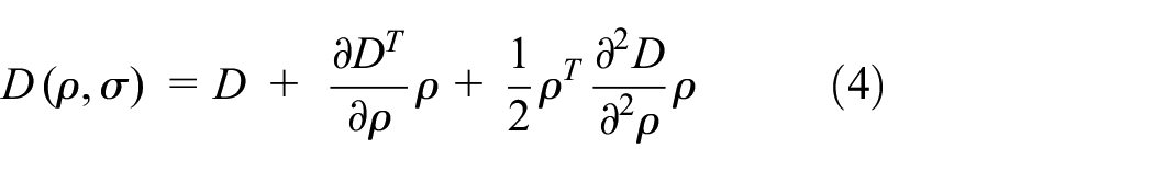
The local extreme of the function D can be detected by accurately localizing the interest points with respect to the proposed method known as Taylor expansion of the scale-space function D (ρ, σ) that is shown in equation (4).

$$D(\rho ,\sigma )=D+\frac{\partial D^T}{\partial \rho }\rho +\frac{1}{2}{\rho }^T\frac{{\partial }^{2}D}{{\partial }^2\rho }\rho$$

(4)

Speeded up robust feature (SURF)

The SURF algorithm which was firstly presented by Bay et al. ¹⁶ is a novel detector and descriptor of scale and rotation invariant interest points. It generates a group of interest points for each image with a set of 128 dimensional descriptors for each point.

In addition to its conceptual similarity to the SIFT, the SURF descriptor likewise focusses on the gradient information distributed space within the interest point neighboring, where the localization and the description of the interest point itself can be done by its detection approaches or in a regular grid. SURF is characterized by its invariance to rotation, scale, brightness and, after reduction to unit length, contrast. That’s why SURF computation is fast and it can increase distinctively, without losing its robustness to rotation of about ± 15°, which is typical for most face recognition tasks. The SURF descriptors are known for their higher robustness compared to the locally operating SIFT descriptors when it comes to dealing with different kinds of image perturbations.

SURF detector interest point localization is based on the Hessian matrix. If a point $\rho =(x,y)$ in an IRT image I, is considered then, the Hessian matrix $H=(\rho ,\sigma )$ at $\rho$ and scale $\sigma$ is written as follows:

$$H=(\rho ,\sigma )=\left[\begin{array}{cc}{L}_{\mathrm{xx}}(\rho ,\sigma )\hfill & L_{\mathrm{xy}}(\rho ,\sigma )\hfill \\ \multicolumn{1}{c}{L_{\mathrm{xy}}(\rho ,\sigma )}& L_{\mathrm{yy}}(\rho ,\sigma )\hfill \end{array}\right]$$

(5)

While $L_{\mathrm{xx}}(\rho ,\sigma )$ is the second order derivative of the Gaussian convolution $\frac{{\partial }^2}{\partial x^2}G(\rho ,\sigma )$ with the image $I$ , and likewise for $L_{\mathrm{xy}}(\rho ,\sigma )$ and $L_{\mathrm{yy}}(\rho ,\sigma )$ .

The SURF is close to second order Gaussian derivatives with box filters named average filter, by contrast the SIFT that is closer to Gaussian Laplacian (LoG) using the Gaussian difference (DoG), this can be rapidly calculated through integral images like shown in Figure 1. The selection of interest point’s location and scale is realized by computing the Hessian matrix determinant. The application of non-maximum suppression in a 3 × 3 × 3 neighborhood allows us to localize the interest points in scale and image space.

Figure 1.

Second order partial derivatives of the Gaussian function and its corresponding box filter.

By using the SURF descriptor, a circular region is constructed around the detected interest point and thus a unique orientation is assigned. Haar wavelet response in both x and y directions is used to compute the orientation, that helps to gain invariance to image rotations. Haar wavelets can be easily calculated by displaying integral images.

The SURF descriptors are created by extracting the square areas around the points of interest when the dominant orientation is evaluated and included in the information on the points of interest. Each windows underlying intensity pattern (first derivatives) is represented by a vector V and each sub-regions are split up in 4 * 4.

$$V=[\sum {\partial }_x,\sum {\partial }_y,\sum |{\partial }_x|,\sum |{\partial }_y|]$$

(6)

Finally, we can summarize the SURF method in four major steps:

• Create the integral image of the supplied input image and calculates pixels sums over upright rectangular areas.

• Construct the Hessian response map determinant, and then localizes a scale space interest points by performing a non-maximal suppression, this results in a localized interest point’s vector. Finally the Hessian Matrix determinant will be used.

• Calculate the interest point dominant orientation and builds a 4 × 4 window around their neighborhood. After that use Haar Wevelet responses from each sub-region and extracts a 128 dimensional descriptor vector based on sums of these Wavelet responses.

• Save each interest point associated data.

Quick distinctive descriptors computation is considered one of the major SURF descriptor advantages. Furthermore, its invariance to common image transformations such as image rotation, scale and illumination changes, and small change in viewpoint makes it more reliable in this task.

Based on what has preceded, it is fairly justified to choose the SURF method as an adopted feature extractor in our experimental work.

Step 2: Histogram of SURF features

The obtained features are encoded as a histogram which represents the occurrence frequency of these visual words. ¹⁷ Before encoding features, k-means clustering^16,22 is used to generate several interest points called vocabulary.

A specified vocabulary size can be obtained by clustering each faulty state extracted features and a set of k; clusters is learned. After that, the centers of the learned clusters are defined as the vocabulary. In this paper, a set of n dimensional vectors of SUFT features (x1, x2, …, xn) is done. Via k-means clustering, the n SUFT vectors are divided into k different groups such that S = {S1, S2, …, Sk} with minimized intracluster squared summed error (SSE), which is done as:

$$S=\arg \underset{s}{min}\sum _i^k\sum _{x\in s_i}\parallel x-u_i{\parallel }^2$$

(7)

Where μi are the mean vector in Si.

Extremely randomized tree (ERT) classifier

In both Random Forest ²³ (RF) and Extremely Randomized Tree ¹⁸ (ERT) based on a great number of decision trees (DT) are used as proper classifiers in order to attain the ultimate classification. These methods consist of four major stages: identification of the input, selection of the optimal number of trees, the analysis of the votes, and the final decision.

There are several differences between Random Forests (RF) and Extremely Random Trees (ERT), of which one can quote. ²⁴

• Unlike the RF, the ERT uses all the training samples to build each decision tree.

• To bifurcate the decision tree, the ERT is completely random, while the RF uses a random subset.

Random forest

RF method was originally developed by Breiman. ²³ It is considered as one of the most successful ensemble learning method. In order to perform a good classification and regression, a great number (hundreds or thousands) of independent decision trees are utilized. Since it is an ensemble methodology, RF employs a number of decision trees as weak classifiers or regressors, combines the concept of bagging, ²⁴ and random feature selection. ²⁵ The RF is a representative ensemble classifier built by a multitude of decision trees. Thanks to its excellent classification accuracy and high efficiency, RF classifier has been attracting increasing attention and wide using domains.

Extremely randomized trees

ERT method ¹⁸ is a group of randomized trees. The ERT maximizes RF algorithm randomization. Just like RF, ERT shows a computational effectiveness and a training capability even when fed with high dimensional input vectors. However, ERT surpasses the RF technique when the training time is taken into account. This rapidity is thanks to a simpler manner to choose the thresholds in ERT. Besides, unlike RF, ERT has a lowers variance that is ensured by its increased randomization. Furthermore, trees in ERT are autonomously trained using the total training data points.

RF and ERT have different core methodologies even if they are both considered as ensemble learning models based on the decision tree algorithm.^18,26 Random forest subsamples the data with replacement. This sub-sampling enriches the data, thereby helping to form the model with highly distinctive learning data.

Oppositely, ERT uses the whole data and hence reduces bias which has a positive impact on the model’s performance. Additionally, both methods have different ways in splitting nodes, RF splits nodes by finding the optimum split while ERT does it randomly. Data variance is lowered in extremely randomized trees by suing this random split. Thereby, both ERT and RF first goal is to ensure an optimal balance of bias and variance. RF and ERT are selected at first place for the reason that their algorithms are based on an ensemble of decision trees. This property gives them a higher performance than the traditional decision tree algorithm.

An ERT classifier is similar to RF but differs in how the randomness is introduced during the training. To train an ERT classifier multiple trees are trained, each tree is trained on all training data. Like the random decision forest, the optimal division at the node level is obtained by analyzing a subset of all available features. Instead of searching for the best threshold for each feature a single threshold for each feature is selected at random. Based on these random divisions, the division that leads to the highest increment in the scale score employed is then selected. The greater degree of randomness through training results in more independent trees and thus reduces the variance further. Due to that extremely randomized trees tend to give better results than random forests.

Experimental work

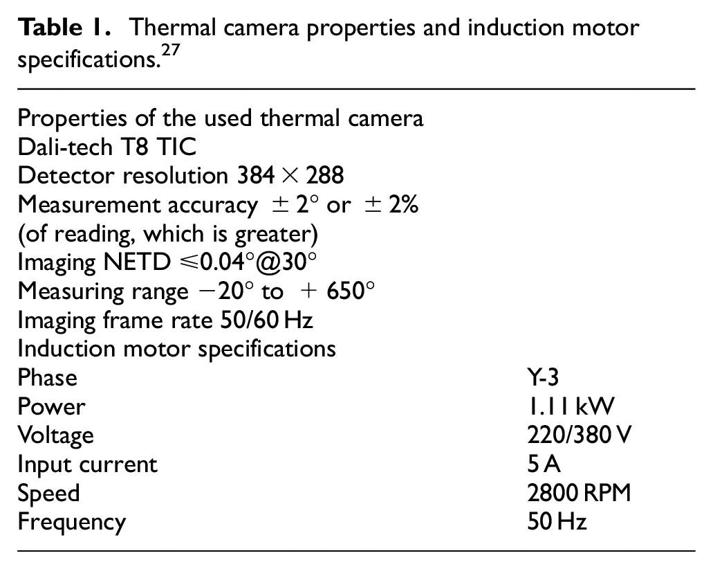
Experiments were conducted on a three phases 1.11 kW, 5 A, 220/230 V. In order to test and train the model, a healthy induction motor and eight different short circuit faults in the stator windings thermal images are captured and considered. All artifact generated defects in this dataset are internal faults, with no relation with external pieces or initial setup electrical components failure. ²⁷

Thermal images acquisition was performed on an Electrical Machines Laboratory workbench by a Dali-tech T4/T8 infrared thermal image camera at an environment temperature of 23°. Thermal camera properties and induction motor specifications are representing in Table 1.

Table 1.

Thermal camera properties and induction motor specifications. ²⁷

Properties of the used thermal camera
Dali-tech T8 TIC Detector resolution 384 × 288 Measurement accuracy ±2° or ±2% (of reading, which is greater) Imaging NETD ≤0.04°@30° Measuring range −20° to +650° Imaging frame rate 50/60 Hz
Induction motor specifications
Phase	Y-3
Power	1.11 kW
Voltage	220/380 V
Input current	5 A
Speed	2800 RPM
Frequency	50 Hz

Nine sets of Images represent a health state and eight different faulty states of the Induction Machine. The %-stator stands for each phase short-circuit rate, while α-phase is the number of phases that contain short-circuit defects as representing in Table 2.

Table 2.

General description of the nine considered states in the induction motor diagnostic.

Stator fault class	0%	50%		30%			10%
α-phase	Healthy	A&B	A	A&B&C	A&C	A	A&B&C	A&C	A
Class label	1	2	3	4	5	6	7	8	9

The thermal images acquisition under healthy and defect conditions are shown in Figure 2. We can clearly notice that the detection and identification of the defect are almost impossible counting only on thermographs direct observation because healthy and faulty conditions thermal images are not distinctive and their differences are not clear which makes bear aye classification misleading and unreliable. This situation made it necessary to research and to develop new machine learning and artificial intelligence methods in order to better differentiate between the studied cases.

Figure 2.

thermal image of induction motor: (a) healthy, (b) 10% in phase A, (c) 10% in phase A&C, (d) 10% in phase A&B&C, (e) 30 % in phase A, (f) 30 % in phase A&C, (g) 30 % in phase A&B&C, (h) 50 % in phase A, and (i) 50 % in phase A&C.

In this context, we propose in this paper a new induction motor condition monitoring method based on extremely randomized trees (ERT) classifier combined with SURF-BoVW features extraction. Figure 3 shows the proposed method flowchart. After the collection of infrared image thermography (IRT), in the first step, features set (visual words) are extracted using the SURF algorithm. Secondly, the histogram is generated after the encoding of the extracted features using the k-mean clustering. Then, the obtained features set are randomly divided into training and testing samples.

Figure 3.

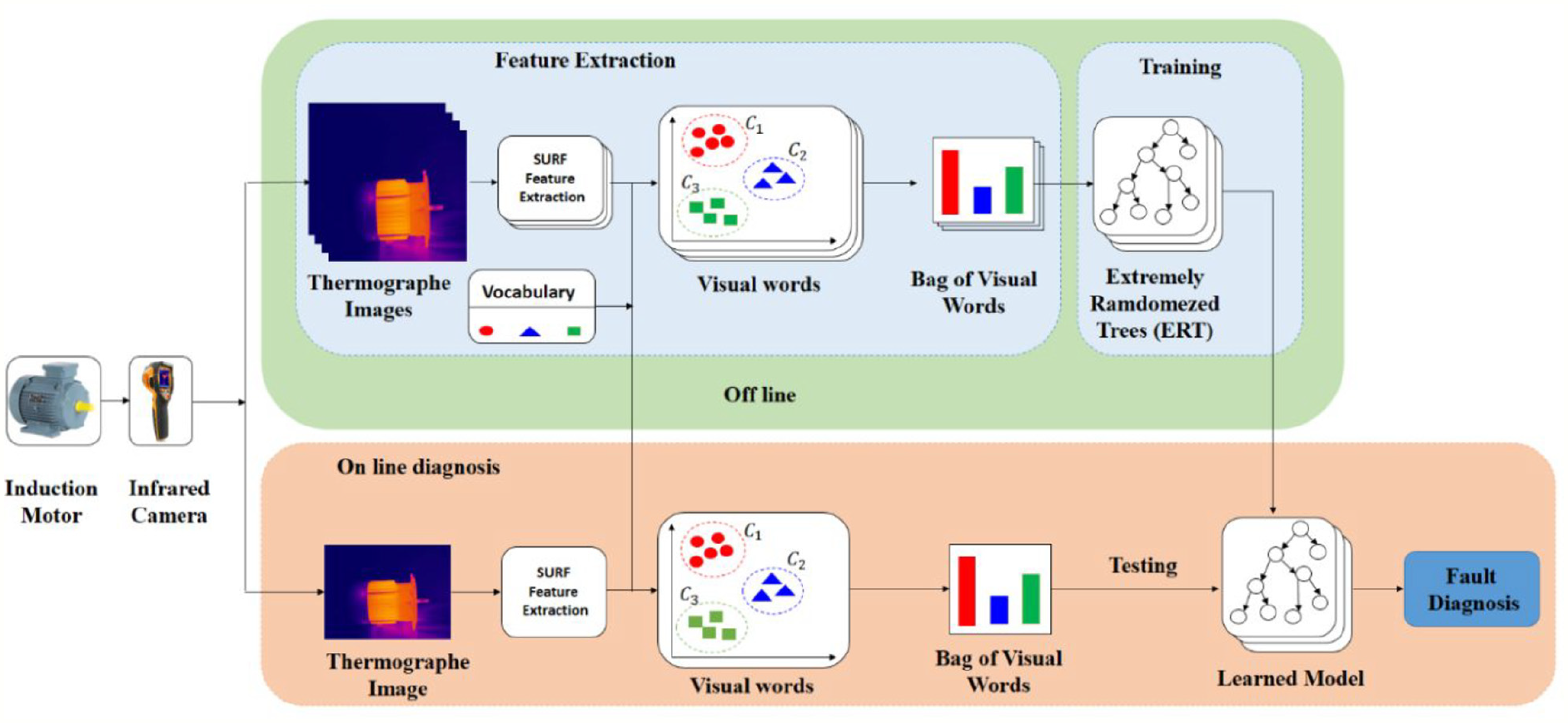
Overview of the proposed method.

Finally, ERT classifier is used for classification. After the training phase is finished and the parameters of the ERT classifier are fixed, the testing samples are classified based on the adopted parameters.

Obtained results and discussion

In the aim to prove the robustness of the adopted method, it is compared with other classification techniques that include KNN, DT, SVM, least squares support vector machine (LSSVM), self-organizing fuzzy logic classifier (SOF), Random Forest (RF), and Deep Rule Based (DRB) respectively.

Moreover, this method’s classification stability had been analyzed based on the standard deviation of 10 experiments. Additionally, the average, maximum, and minimum values are taken to reduce the impact of the contingency.

All the above mentioned classification methods consider the features set extracted by BOVW and SURF as an input. In standard SVM, the penalty factor equals to 100, and the kernel function is 0.01. DTs minimum number of father nodes is 5. K = 5 is taken as the nearest neighbor number of KNN. The Gaussian kernel function of the LSSVM is 0.5, and its regularization parameter is 10,000.

The obtained results from each classification method are represented in Table 3.

Table 3.

Obtained classification results of the tested methods.

	KNN	SOF	ERT	DT	SVM	LSSVM	RF	DRB
Max	0.9815	1.0000	1.0000	1.0000	1.0000	1.0000	1.0000	1.0000
Min	0.8796	0.9444	1.0000	0.9259	0.8981	0.9630	0.9815	0.9537
Mean	0.9466	0.9779	1.0000	0.9786	0.9843	0.9879	0.9972	0.9815
Std	0.0293	0.0171	0.0000	0.0260	0.0308	0.0138	0.0070	0.0169

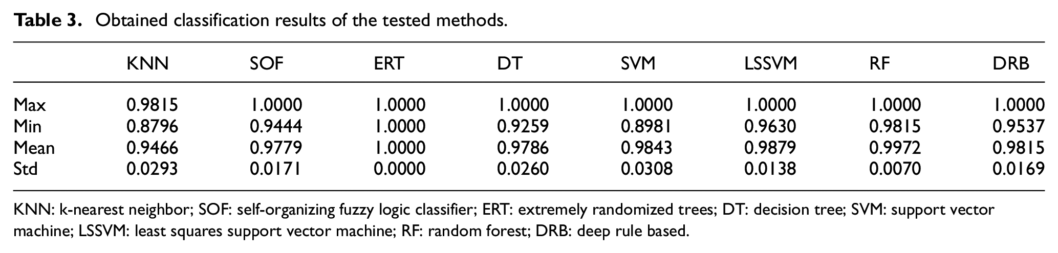
KNN: k-nearest neighbor; SOF: self-organizing fuzzy logic classifier; ERT: extremely randomized trees; DT: decision tree; SVM: support vector machine; LSSVM: least squares support vector machine; RF: random forest; DRB: deep rule based.

Table 3 illustrates the low classification accuracy of KNN compared to the other methods. In addition to that, the standard deviation revealed the unsteadiness classification effect of this method on different testing samples, and the instability of its classification algorithm.

KNN is lower than SVM both in the average classification accuracy and its standard deviation by 3.7700% and 0.0015 successively. The SVM standard deviation classification accuracy is 0.0308. However its algorithm is unstable, with a 10.2 % lower minimum classification accuracy than that of ERT.

The maximum classification accuracy of SOF, DT, SVM, LSSVM, RF, and DRB is 100%, but the standard deviation of classification accuracy are higher than that of ERT classifier. The classification accuracy is greatly influenced by the input of different samples in SOF, DT, LSSVM, RF, and DRB.

Compared to ERT, the average classification accuracy of RF is considerably significant. Even so, if we focus on the standard deviation of classification accuracy, the RF classification stability is not as good as the proposed method.

Globally, the classification accuracy of our method is the highest of all the tested methods. Consequently, its classification result is the best and the most reliable.

In order to offer an intuitive illustration of the classification effects resulting from various methods, Figures 4 and 5 respectively shows the confusion matrix and classification results of the previously discussed methods in the eighth experiment.

Figure 4.

Confusion matrix of each classification method in the eighth experiment: (a) confusion matrix of KNN, (b) confusion matrix of ERT, (c) confusion matrix of SOF, (d) confusion matrix of DT, (e) confusion matrix of SVM, (f) confusion matrix of LSSVM, (g) confusion matrix of RF, and (h) confusion matrix of DRB.

Figure 5.

Classification results of each classification method in the eighth experiment: (a) classification results of KNN, (b) classification results of ERT, (c) classification results of SOF, (d) classification results of DT, (e) classification results of SVM, (f) classification results of LSSVM, (g) classification results of RF, and (h) classification results of DRB.

From the figure of the KNN confusion matrix, we can see that the KNN has the lowest classification accuracy which equals 93.2099%, and we can also clearly see that the KNN has a misclassification in categories 2nd, 3rd, 7th, and 8th. So that around 8.7% of the test samples are misclassified for the second category, 15.79% and 23.53% of the test samples for the third and seventh category respectively, and 11.76% of the samples are misclassified for the category 8.

In the classification results of KNN, 6.7901% of testing samples are misclassified, of which 8.7% of category 2 are classified as category 4 and 9 equally, 15.79% of category 3 are classified as category 8, 23.53% of category 7 are classified as category 5 by 17.66% and category 1 by 5.882%, and 11.76% of category 8 are classified as category 3.

A total of 1.2346% samples in the classification results of SOF and DRB are misclassified, however, for SOF classifier there are 4.348% of category 1 are classified as category 7 and 5.263% of category 4 are considered as category 2. On the other hand, in the case of DRB 5.263% of category 3 are classified as category 8, and 5.882% of category 7 are considered as category 5.

A total of 0.6173% samples in the classification results of LSSVM are misclassified, where 5.88% of category 7 are considered as category 6. On the other hand, in the case of DT classifier a total of 3.7037% are misclassified, where 23.53 of category 8 are classified as category 3 and 9.524% of category 9 are considered as category 4.

A total of 1.2346 % samples in the classification results of SVM and RF classifiers are misclassified, however, for SVM classifier there are 10.53% of category 3 are classified as category 9, on the other hand, in the case of RF 11.76% of category 8 are classified as category 3.

In the classification results of proposed method (ERT), there are no misclassified samples, and the classification accuracy is 100%.

Furthermore, the evaluation of this experiment’s results from different perspectives is performed using polygon Area Metric (PAM).

Classification evaluation using polygon area metric

In order to assess a single scale classifier’s performance, Polygon Area Metric ²⁸ is a novel method that is used thanks to its stability and its profound measure.

Six existing metrics including CA, SE, SP, AUC, JI, and FM are used to create a polygon, then the corresponding area for PAM is calculated. The theoretical formulas are mentioned bellow:

$$\begin{array}{c}\mathrm{Classification}\mathrm{Accuracy}\hfill \\ =\mathrm{CA}=\frac{\mathrm{TP}+\mathrm{TN}}{\mathrm{TP}+\mathrm{TN}+\mathrm{FP}+\mathrm{FN}}\hfill \end{array}$$

(8)

$$\mathrm{Sensitivity}=\mathrm{SE}=\frac{\mathrm{TP}}{\mathrm{TP}+\mathrm{FN}}$$

(9)

$$\mathrm{Specificity}=\mathrm{SP}=\frac{\mathrm{TN}}{\mathrm{TN}+\mathrm{FP}}$$

(10)

$$\mathrm{Jaccard}\mathrm{Index}=\mathrm{JI}=\frac{\mathrm{TN}}{\mathrm{TN}+\mathrm{FP}}$$

(11)

$$\mathrm{F}-\mathrm{measure}=F=\frac{2\mathrm{TP}}{2\mathrm{TP}+\mathrm{FP}+\mathrm{FN}}$$

(12)

$$\mathrm{Area}\mathrm{Under}\mathrm{Curve}=\mathrm{AUC}={\int }_0^{1}f(x)\mathrm{dx}$$

(13)

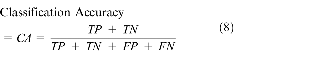
Where TP, TN, FP, and FN are respectively known as the correctly predicted positive and negative samples numbers, and the incorrectly predicted positive and negative samples ones.

The true-positive rate (SE) plot in function of the false-positive rate (1-SP) for different cut-off points R represents the receiver operating characteristic curve f(x). It should be known that SE and SP respectively refer to the ratios of correctly classified class 1 and class 2 samples total population.

As illustrated in Figure 6, the PAM calculation is done using the polygon’s area created by CA, SE, SP, AUC, JI, and FM points in a regular hexagon. It worth noting that the regular hexagon is made up of 6 equilateral triangles and each side length is equal to 1. Therefore, it is fair to say that |OP₁| = |OP₂| =|OP₃| = |OP₄| = |OP₅| = |OP₆| = 1, with an area of 2.59807.

Figure 6.

Polygon in regular hexagon. ²⁵

|OP₁|, |OP₂|, |OP₃|, |OP₄|, |OP₅|, and |OP₆| lengths respectively are the values of CA, SE, SP, AUC, JI, and FM. The calculation of the PAM is done based on the following formula:

$$\mathrm{PAM}=\frac{\mathrm{PA}}{2.59807}$$

(14)

PA is the polygon’s area.

It should be mentioned that the normalization of the PAM into the [0, 1] interval is ensured by dividing the PA value by 2.59807.

Figure 7 shows the visual results of Polygon area metric of each classification method in the eighth experiment.

Figure 7.

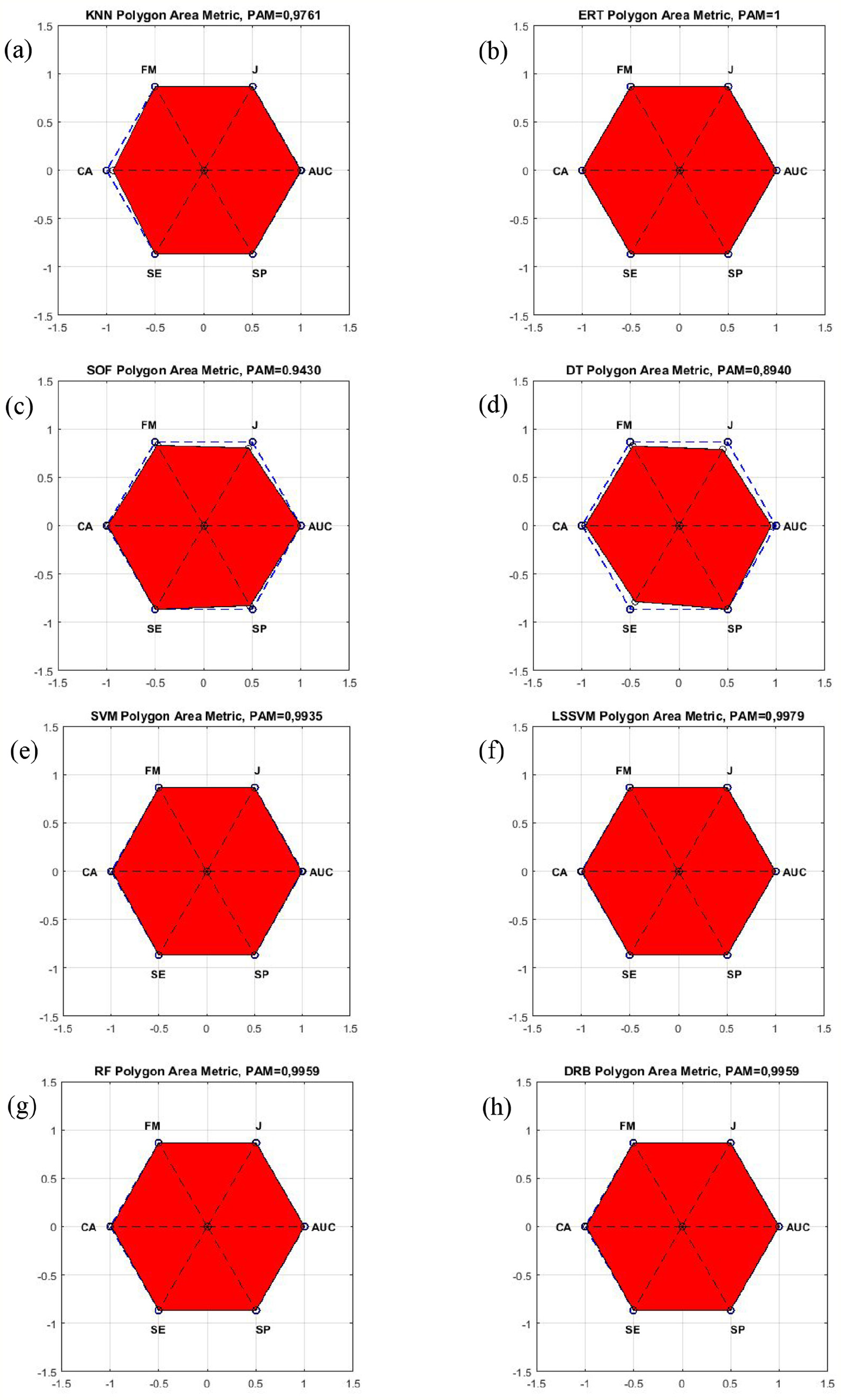
Polygon area metric graphs of each classification method in the eighth experiment: (a) polygon area metric of KNN, (b) polygon area metric of ERT, (c) polygon area metric of SOF, (d) polygon area metric of DT, (e) polygon area metric of SVM, (f) polygon area metric of LSSVM, (g) polygon area metric of RF, and (h) polygon area metric of DRB.

From these visual graphs, it can be observed among the PAM covered areas of all the tested classification methods, ERT has largest area, followed by that of the RF classifier.

Conclusion

A new induction motor fault diagnosis method based on SURF-BoVW and ERT classifier is proposed in this paper to diagnose various faults of induction motors. The IRT-based method is proven to be effective noncontact, nonintrusive, high sensitive, and stable to various faults.

The efficiency of the proposed method is validated by identifying eight sorts of induction motor stator faults (the rate of short-circuit in each phase and the number of phases included faulty phases in the induction motor).

Under the premise of the same input, the ERT classifier is always higher than that of RF, and the classification effect is better and stable. By comparing it with SVM, DT, KNN, LSSVM, and DRB, the ERT classifier had demonstrated the highest classification accuracy, stability, and the best fitted to be used in the diagnosis of induction motor faults, since its classification precision had reached 100%.

In order to evaluate the proposed method, polygon Area Metric (PAM) is used. The obtained results clearly show that the ERT Polygon Area Metric followed by the rest of the classifiers.

Compared to other existing classification methods, the obtained experimental results using ERT classifier indicate that the proposed method can be considered as a reliable alternative to monitor the state of an induction motor.