Sage Journals: Discover world-class research

Abstract

In the previous models of rolling bearings with a single fault, the displacement deviation caused by the collision of the fault to the rolling element changes instantly. However, the displacement deviation should change gradually. Here, the asymptotic idea is introduced to describe the change of the displacement deviation. The calculation method of the deviation is given. An asymptotic model of rolling bearings with an inner raceway fault is constructed. Then, the simulation of the SKF6205 bearing with a single fault is carried out. The differences between the previous model and the asymptotic model for the responses and the displacement deviation are compared. The effects of the speed and fault size on the dynamic characteristics are analyzed. Finally, the experiments are carried out to corroborate the rationality of the constructed model. The research results can provide theoretical support for the dynamic analysis, fault diagnosis, and reliability analysis of rolling bearings.

Keywords

Dynamic model inner raceway rolling bearings single fault displacement deviation

Introduction

Rolling bearing is an essential part of supporting and rotation in the rotating machinery. Due to the worse working environment, rolling bearings always inevitably suffer from faults, resulting in vibration and noise of the mechanical equipment. Therefore, it is necessary to study the fault mechanism and dynamic model of rolling bearing.

More recently, the improvement on the model of rolling bearings has been carried out to study its dynamic characteristics. A dynamic model of the inner raceway with six freedom degrees was provided by Sopanen and Mikkola.^1,2 Bearing shape, material properties, and the radial gap was included in this model. To predict the vibration of ball bearings with a single fault in the inner raceway, Shah and Patel³ proposed a model including weights of shaft, raceway, ball, and housing, stiffness, damping, and lubrication films. Rafsanjani et al.⁴ prepared an analysis model for characterizing the nonlinear dynamic behaviors of the inner raceway with a surface defect. He also derived a mathematical formula for the defect to evaluate the impacts of radial clearance and contact force. Zhao et al.⁵ described a modeling method for the inner raceway by analyzing the interaction between balls and all raceways. And he studied the effects of fault size, fault position, and fault number on the nonlinear dynamic behaviors by phase diagrams, orbit diagrams, and frequency spectrograms. Considering the rolling element position and fault position in three dimensions, an improved model of rolling bearings with a single fault in the inner raceway was proposed by Jiang et al.⁶ Then, the vibration responses caused by a sudden change in contact force were studied based on the model. Luo et al.^7,8 explored the nonlinear excitation mechanism of the double-impact phenomenon caused by a fault in ball bearings and proposed a dynamic model to describe the phenomenon. Considering nonlinear factors such as oil film and rolling element sliding, Zhang and Lv⁹ proposed an improved model of rolling bearings with a pitting fault in the inner raceway. In view of the vibration caused by a fault in the inner raceway under radial load, Chang et al.¹⁰ refined the contact process of the rolling element with the fault into multiple events and proposed a model with two freedom degrees. Considering the centrifugal force and gyro moment of rolling elements at high speed, a five freedom-degrees model of rolling bearings with an inner raceway fault was proposed by Qin et al.¹¹ Gao et al.¹² presented a model of inter-shaft bearings with a single fault in the outer raceway or inner raceway and investigated the nonlinear characteristics of rolling bearings affected by the defect. To better understand the vibration characteristics of rolling bearings with faults is critical for the diagnosis, a dynamic model is proposed by Niu et al.¹³ Slippage, rolling element dimension, and the change of contact force direction were included in this model. Considering the frictional force and contact force between rolling elements and raceways, a model was provided to study the vibration response of the cylindrical roller bearing.¹⁴ The interaction between the frictional force and the response of rolling bearings was included in the proposed model when a skidding happens.

From the preceding discussion, the fault of rolling bearings is treated as a regular rectangle. However, the fault can be the other shapes.¹⁵ A method characterizing the irregular bearing fault was introduced into modeling of rolling bearings by Wang et al.¹⁶ The vibration responses of the rolling bearings with a fault were analyzed by numerical calculation. The influence of the circumferential width and depth of the fault on the system vibration was studied when the bearings contain a rectangular fault or an irregular fault in the inner raceway. Sawalhi and Randall^17,18 characterized the change of the interval by a function that the fault depth changes in a cone with the rotation angle. The fine modeling of rolling bearings with a fault was realized by the function. Aiming at the modeling problem of rolling bearings in an aeroengine rotor system, Chen¹⁹ described the bearing local fault by the semicircular groove to improve the morphology of the fault. Although the fault is considered to be irregular, the displacement deviation caused by the collision of rolling elements to the fault is still believed to release or restore immediately. That is, the displacement deviation will be released if a rolling element rolls into the fault region. And the value of the displacement deviation is considered to be equal to the fault depth.

To solve the main problems in the current research, a novel model of rolling bearings with a single fault in the inner raceway is proposed considering the asymptotic change of the displacement deviation. The change rule and the specific calculation method of the deviation are explored. The differences between the transient model and the asymptotic model are analyzed. The models of rolling bearings with different speeds and different fault sizes are discussed.

The content of the remaining chapters can be divided into four main parts. In Section 2, the asymptotic model of rolling bearings with a single fault in the inner raceway is developed. In Section 3, the correctness of the asymptotic model is validated by the numerical simulation. The differences and similarities between the transient model and the asymptotic model are studied. In Section 4, the correctness of the established model is verified by experiments. In section 5, some valuable conclusions are drawn.

Presentation of the asymptotic model

Figure 1(a) shows the transient model.²⁰ The fault is simplified into a rectangular groove in the model. Once a rolling element contacts the fault, the displacement deviation changes immediately. However, the fault can be an arc groove shown in Figure 1(b), and the displacement deviation changes gradually.

Figure 1.

Fault models of rolling bearings: (a) transient model and (b) asymptotic model.

Figure 2 shows the asymptotic model of rolling bearings with a single fault in the inner raceway.

Figure 2.

Asymptotic model of rolling bearings.

In Figure 2, ω_i represents the rotational speed of the inner raceway, D_m represents the pitch diameter, θ_spall represents the initial azimuth angle of fault, D_b represents the diameter of rolling elements, and R_i represents the radius of the inner raceway.

The span angle ΔΦ_s of the fault can be calculated by

Δ Φ_{s} = 2 \arcsin \frac{b_{c}}{R_{i}} \approx \frac{2 b_{c}}{R_{i}}

(1)

where b_c represents half the fault width.²¹

Since the inner raceway rotates with the shaft at high speed, the azimuth angle θ_s of the fault changes continuously. The variation process of the azimuth angle can be written as

θ_{s} = ω_{i} t + θ_{spall}

(2)

Figure 3 shows the contact between a rolling element and the fault.

Figure 3.

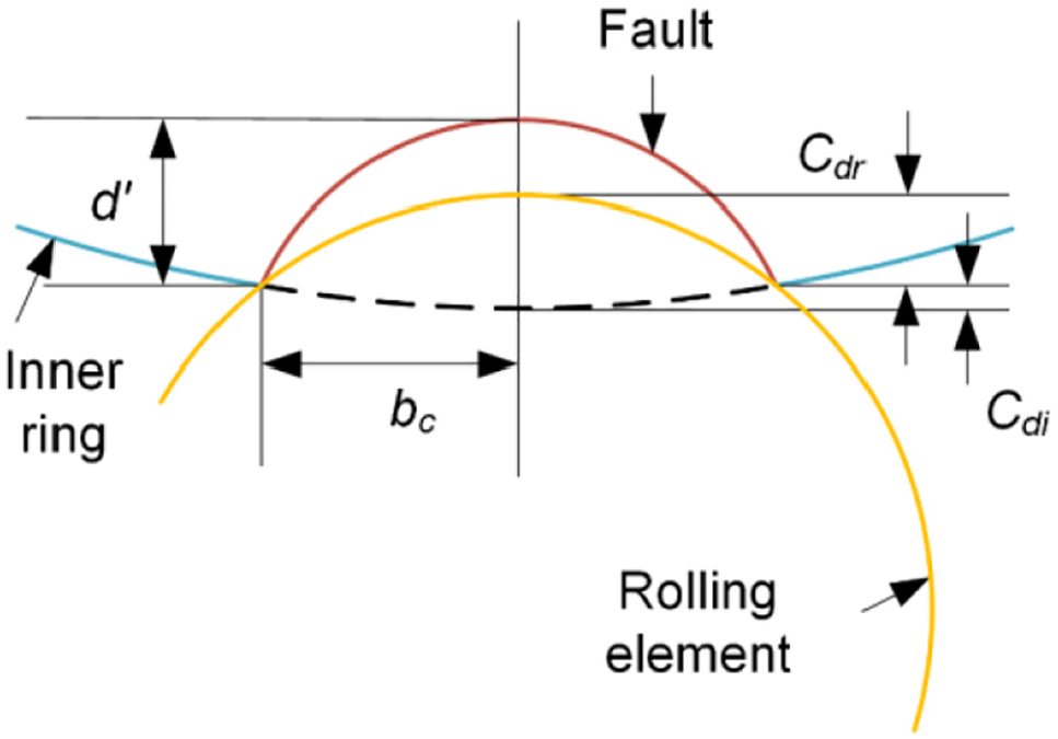
The contact between a rolling element and the fault.

In Figure 3, d′ represents the fault depth, C_dr and C_di represent the deviation of the rolling element and that of the inner raceway, respectively. From Figure 3, the maximum deviation λ_max should be written as

λ_{max} = C_{dr} + C_{di}

(3)

C_{dr} = \frac{D_{b}}{2} - \sqrt{{(\frac{D_{b}}{2})}^{2} - b_{c}^{2}}

(4)

C_{di} = R_{i} - \sqrt{{(R_{i})}^{2} - b_{c}^{2}}

(5)

Since the fault is an arc groove, the rolling element should roll asymptotically in the fault span, that is, the displacement deviation should gradually change. Therefore, the deformation can be written as

λ = λ_{max} - R_{i} * [1 - \cos (θ_{s} - θ_{j})]

(6)

where θ_j represents the azimuth angle of the jth rolling element.

According to Hertz theory, the contact between rolling elements and raceways is simplified into a pair of spring-damping models shown in Figure 4.^22,23

Figure 4.

Contact model.

According to the contact model, the spring load Q_j produced by the point contact between the jth rolling element and raceways can be written as

Q_{j} = K \times δ_{j}^{3 / 2}

(7)

K = 1 / [(1 / K_{o})^{2 / 3} + (1 / K_{i})^{2 / 3}]^{3 / 2}

(8)

where K represents the total load-deflection constant, δ_j represents the contact deformation of the jth rolling element, and K_o and K_i represent the contact stiffness of the outer raceway and that of the inner raceway, respectively.²⁴ For ball bearings, the stiffness can be calculated by

K_{o} (K_{i}) = 2.15 \times 10^{5} \times (Σ ρ)^{- 1 / 2} (n_{δ})^{3 / 2}

(9)

where Σρ is the sum of contact principal curvature and n_δ is a coefficient related to the difference function.²⁵

For a normal bearing without defect, the contact deformation of the jth rolling element can be calculated by

δ_{j} = x \cos θ_{j} + y \sin θ_{j}

(10)

θ_{j} = ω_{c} t + \frac{2 π (j - 1)}{Z} + θ_{1}

(11)

ω_{c} = \frac{1}{2} [ω_{i} (1 - \frac{D_{b}}{D_{m}} \cos α)]

(12)

where ω_c represents the angular acceleration of the cage, Z represents the number of rolling elements, θ₁ represents the azimuth angle of the 1st rolling element, and α represents the contact angle.²⁶

Considering the influence of the displacement deviation λ, the total contact deformation can be calculated by

δ_{j} = x \cos θ_{j} + y \sin θ_{j} - β_{j} λ

(13)

β_{j} = {\begin{matrix} 1 & θ_{s} - \frac{Δ Φ_{s}}{2} < θ_{j} < θ_{s} + \frac{Δ Φ_{s}}{2} \\ 0 & others \end{matrix}

(14)

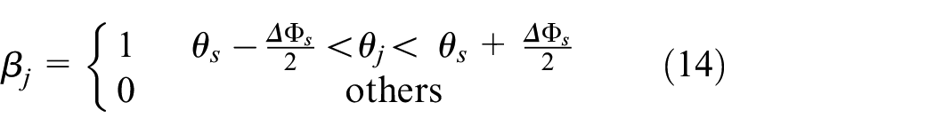
where β_j is a switch function.²⁷ The function indicates that the displacement deviation exists if the rolling element rolls into the fault span. Otherwise, the displacement deviation no longer exists.

The total spring load is obtained by adding all the spring loads and projecting on the X-axis and Y-axis,²⁸ that is,

{\begin{matrix} Q_{x} = \sum_{j = 1}^{Z} (Q_{j} \cdot \cos θ_{j}) \\ Q_{y} = \sum_{j = 1}^{Z} (Q_{j} \cdot \sin θ_{j}) \end{matrix}

(15)

The dynamics equations of rolling bearings with a single fault in the inner raceway are written as

{\begin{matrix} m x^{″} + c x^{'} + Q_{x} = F_{r} + F_{e} \cdot \cos ω_{i} t \\ m y^{″} + c y^{'} + Q_{y} = F_{e} \cdot \sin ω_{i} t - mg \end{matrix}

(16)

where m represents the weight of rolling bearings, c is the equivalent coefficient of damping, F_r represents a radial load, and F_e represents an external load.

Simulation analysis

Here, the simulations of SKF 6205 bearing are carried out. The main parameters of the bearing are described below. m = 0.13 kg, R_i = 25 mm, D_b = 7.94 mm, Z = 9, α = 0°. The initial displacements and speeds are x = y = 0 mm and x′ = y′ = 0 mm/s. The equivalent coefficient of damping is 200 N s/m.

The established model is solved by the Runge-Kutta (4, 5) pair that comes with MATLAB. And the frequency signal is obtained according to the FFT method.

Differences between the transient model and the asymptotic model

In this section, the rotational speed n_i is 1772 rpm. The characteristic frequencies of the shaft speed and the fault can be calculated by

F_{S} = \frac{n_{i}}{60} \approx 29.53 Hz

(17)

F_{i} \approx 5.42 \cdot F_{S} \approx 160.07 Hz

(18)

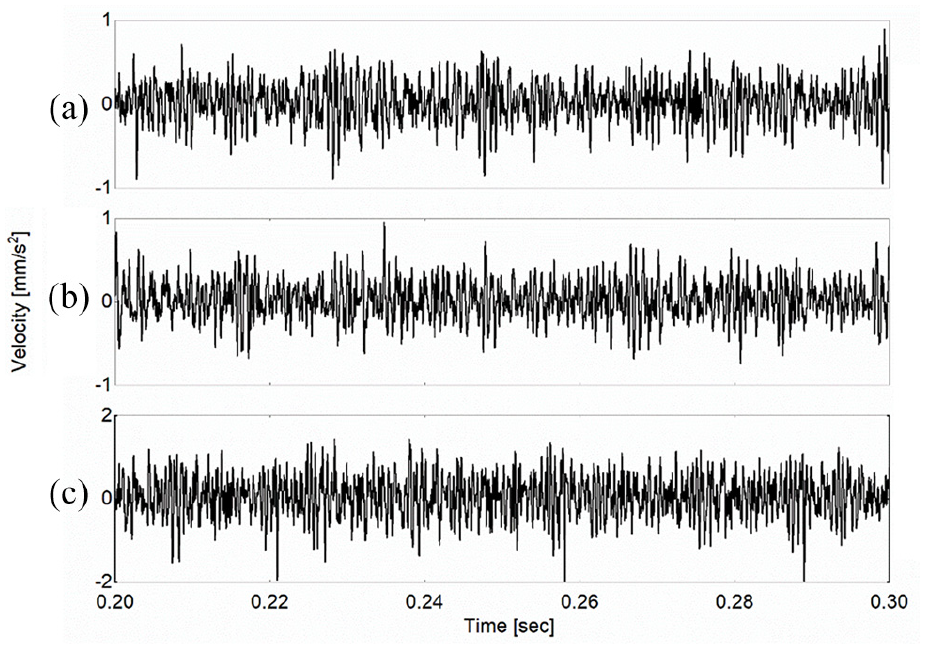
First, rolling bearings without any faults are simulated. Figures 5 and 6 show time-domain responses and frequency responses of rolling bearings, respectively.

Figure 5.

Time-domain responses of rolling bearings without any faults: (a) velocity responses for the horizontal direction, (b) velocity responses for the vertical direction, (c) acceleration responses for the horizontal direction, and (d) acceleration responses for the vertical direction.

Figure 6.

Frequency responses of rolling bearings without any faults: (a) velocity responses for the horizontal direction, (b) velocity responses for the vertical direction, (c) acceleration responses for the horizontal direction, and (d) acceleration responses for the vertical direction.

Both velocity responses and acceleration responses in the time-domain are quasi-periodic signals with three periods in 0.1 s. So, the response frequency is 30 Hz corresponding to F_s shown in all the frequency responses. These results confirm the fact of the rolling bearing without any faults.

Then, rolling bearings with a single fault in the inner raceway are simulated. A local fault with a depth of 0.28 mm and a width of 0.18 mm is set in the simulation. To analyze the differences between the transient model and the asymmetric model, all the two models are simulated. Figures 7 and 8 are the comparison charts of responses obtained based on the two models.

Figure 7.

Time-domain responses of rolling bearings based on the two models: (a) velocity responses for the horizontal direction, (b) velocity responses for the vertical direction, (c) acceleration responses for the horizontal direction, (d) acceleration responses for the vertical direction, (e) one impact process in Figure 7(c), and (f) one impact process in Figure 7(d).

Figure 8.

Frequency responses of rolling bearings based on the two models: (a) velocity responses for the horizontal direction, (b) velocity responses for the vertical direction, (c) acceleration responses for the horizontal direction, and (d) acceleration responses for the vertical direction.

From Figure 7(a) and (b), the velocity responses for the horizontal direction and vertical direction show the same periodic characteristics as those of rolling bearings without any faults. Compared with the responses from the asymptotic model, those from the transient model show the impact phenomenon. From Figure 7(c) and (d), the acceleration responses for the horizontal direction and vertical direction are obviously different from those of rolling bearings without any faults. The acceleration responses of the transient model contain 16 impact peaks in 0.1 s. Therefore, the response frequency is 160 Hz corresponding to F_i. Comparing with the acceleration responses of the transient model, those of the asymptotic model don’t fluctuate significantly. One of the impacts is selected to observe the change of the acceleration responses more clearly. Therefore, Figure 7(e) and (f) are drawn. Amazingly, the peaks also appear in the acceleration responses of the asymptotic model. However, the peak is obviously lower than that of the transient model. This result proves that the displacement deviation in the asymptotic model is less than that in the transient model.

From Figure 8, the F_i and 2F_i of all the responses are obvious. And the F_S in the velocity frequency response is more obvious than that in the acceleration frequency response. This result also proves that the periodic characteristics of the velocity response are more obvious than that of the acceleration response. The values of F_S in the asymptotic model are almost the same as those in the transient model, but the values of F_i are smaller.

Finally, we also compare the changes in displacement deviation λ of the two models during the calculation process. Only the impact process shown in Figure 7(e) and (f) is compared for clarity.

From Figures 9, λ in the transient model has an obvious change. From the local enlarged picture of λ in the transient model, λ suddenly jumps to a high level and remains high throughout the impact. From the local enlarged picture of λ in the asymptotic model, the change of λ is a circular arc, and the value of λ is smaller than that in the transient model. The results are in line with the previous analysis for the two models.

Figure 9.

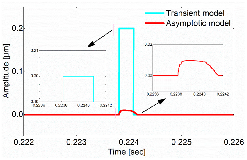
The displacement deviation of the two models during one impact process.

The influence of speed on the dynamic characteristics of rolling bearings

In this section, rolling bearings with a fault in the inner raceway are simulated at different speeds. The fault width is 0.18 mm, and the fault depth is 0.28 mm. The speed is set to 1000, 2000, 3000, 4000, and 5000 rpm, respectively. From Figures 7 and 8, the acceleration responses can better show the differences between the two models compared with the velocity responses. Therefore, in the following research, only the vertical acceleration responses are given. Figures 10 and 11 are the responses of the two models under different speeds.

Figure 10.

Time-domain responses of the two models under different speeds: (a) 1000 rpm, (b) 2000 rpm, (c) 3000 rpm, (d) 4000 rpm, and (e) 5000 rpm.

Figure 11.

Frequency responses of the two models under different speeds: (a) 1000 rpm, (b) 2000 rpm, (c) 3000 rpm, (d) 4000 rpm, and (e) 5000 rpm.

From Figure 10, the responses of the asymptotic model don’t fluctuate significantly comparing with those of the transient model. With the increase of speed, the periodic characteristics of the responses from the two models become more and more obvious. This character is also reflected in the amplitude of F_S shown in Figure 11, that is, the amplitude of F_S also increases with the increase of the rotational speed. When the speed reaches 4000 rpm, the amplitude of F_S exceeds that of F_i. It shows that the frequency of the rotating speed will cover up the fault frequency. This is one of the reasons why the fault is difficult to be diagnosed when rolling bearings run at a high speed.

The influence of fault size on the dynamic characteristics of rolling bearings

In this section, rolling bearings with different fault sizes are simulated at 1772 rpm. The fault width is set to 0.18, 0.36, and 0.53 mm, respectively. The fault depth is 0.28 mm. Figures 12 and 13 are the responses of the two models with different fault sizes.

Figure 12.

Time-domain responses of the two models with different fault widths: (a) 0.18 mm, (b) 0.36 mm, and (c) 0.53 mm.

Figure 13.

Frequency responses of the two models with different fault widths: (a) 0.18 mm, (b) 0.36 mm, and (c) 0.53 mm.

From Figure 12, the responses of the transient model don’t fluctuate significantly. For the responses of the asymptotic model, the impact peaks are beginning to appear and the peak value increases with the enlargement of fault width. This characteristic is also reflected in the amplitude of F_i and 2F_i shown in Figure 11. The amplitudes of F_i and 2F_i increase with the enlargement of fault width. That is, the smaller the fault width, the smaller the amplitude of the fault frequency. This result explains why the small fault is difficult to be diagnosed. The growth rates of F_i and 2F_i are almost the same in the transient model. However, the growth rate of 2F_i is higher than that of F_i in the asymptotic model.

Experiment analysis

In this section, the experiments were carried out to verify the correctness of the simulation results. Here, the sample data of rolling bearings from Bearing Data Center are used.²⁹ The experimental equipment is shown in Figure 14. The equipment is mainly composed of a motor on the left, a torque transducer/encoder on the middle, a power meter on the right, and a control device. Accelerometers were placed at the 12 o’clock position at the fan end of the motor housing. The type of rolling bearings in the experiment is the same as that in the simulation. Vibration data were collected by accelerometers at 48,000 samples per second. A single fault was introduced into rolling bearings by electro-discharge machining.

Figure 14.

The experimental equipment.

First, the responses of rolling bearings at different speeds are studied. Here, the fault width is 0.18 mm, and the fault depth is 0.28 mm. The speed is set to 1730, 1750, and 1797 rpm, respectively. Figures 15 and 16 are the responses of rolling bearings in the experiment.

Figure 15.

Time-domain responses of the experimental results at different speeds: (a) 1730 rpm, (b) 1750 rpm, and (c) 1797 rpm.

Figure 16.

Frequency responses of the experimental results at different speeds (a) 1730 rpm, (b) 1750 rpm, and (c) 1797 rpm.

From Figure 15, the time-domain responses do not change significantly with the increase of speed. The periodic characteristic doesn’t show up in the time-domain responses. The possible reason is the smaller speed interval. From Figure 16, with the increase of the speeds, the value of F_s grows by a small margin, but the values of F_i and 2F_i do not change. This result is consistent with that of the asymptotic model and the transient model.

Then, the responses of rolling bearings with different fault widths are studied at 1730 rpm. Here, the fault width is set to 0.18, 0.36, and 0.53 mm, respectively. Figures 17 and 18 are the time-domain responses and frequency responses of rolling bearings with different fault widths in the experiment.

Figure 17.

Time-domain responses of the experimental results with different fault widths: (a) 0.18 mm, (b) 0.36 mm, and (c) 0.53 mm.

Figure 18.

Frequency responses of the experimental results with different fault widths: (a) 0.18 mm, (b) 0.36 mm, and (c) 0.53 mm.

From Figure 17, the time-domain responses do not change significantly with the enlargement of fault width. The impact peak doesn’t show up either. From Figure 18, the changes in the amplitude of F_s and F_i are not obvious. The value of 2F_i grows by a small margin with the increase of speed. This result is consistent with that of the proposed asymptotic model. Therefore, the correctness of the proposed asymptotic model is proved.

Conclusions

In this paper, the asymptotic concept was introduced to describe the change of the deformation deviation. Then, the asymptotic model of rolling bearings with a single fault in the inner raceway was proposed. The similarities and differences between the transient model and the asymptotic model were studied. The variation rule and specific calculation method of the deformation deviation were given. The following conclusions were obtained.

Obvious shock phenomena can be seen in the time-domain responses from the transient model, and its reflection in the frequency responses is that the amplitude of the fault frequency is significantly higher than that of the rotating frequency. The time-domain responses from the asymptotic model do not show obvious impact phenomena, and the amplitude of fault frequency is lower than that of the rotating frequency. Comparing with the experimental responses of rolling bearings with a single fault in the inner raceway, the responses from the asymptotic model are more consistent with the experimental results. Therefore, the asymptotic model proposed in this paper is reasonable.

As the speed increases, the periodic characteristic of the time-domain responses becomes more and more obvious, and its reflection in the frequency responses is that the amplitude of the rotating frequency gradually increases. When the speed is high enough, the amplitude of the rotating frequency will exceed that of the fault frequency. This result explains why faults of rolling bearings are difficult to be diagnosed at high speeds.

As the size of the fault increases, the impact peak begins to appear in the time-domain responses from the asymptotic model and the amplitude of the peak increases. The amplitudes of the fault frequency and its double frequency also increase. This result explains why the small fault is difficultly diagnosed.

Footnotes

Appendix

Handling Editor: Chenhui Liang

Author contributions

ZL was in charge of the whole trial, YL wrote the manuscript, and JT and DT assisted with sampling and laboratory analyses. All authors read and approved the final manuscript.

Declaration of conflicting interests

The author(s) declared no potential conflicts of interest with respect to the research, authorship, and/or publication of this article.

Funding

The author(s) disclosed receipt of the following financial support for the research, authorship, and/or publication of this article: This work supported by the grant from National Natural Science Foundation of China (Grant Nos. 52075236, 51675258), State Key Laboratory of Mechanical System and Vibration (No. MSV201914), and Laboratory of Science and Technology on Integrated Logistics Support, National University of Defense Technology (Grant No. 6142003190210).

ORCID iD

Yunlong Li

References

Sopanen

Mikkola

Dynamic model of a deep-groove ball bearing including localized and distributed defects. Part 1: theory. Proc IMechE, Part K: J Multi-body Dynamics 2003; 217: 201–211.

Sopanen

Mikkola

Dynamic model of a deep-groove ball bearing including localized and distributed defects. Part 2: implementation and results. Proc IMechE, Part K: J Multi-body Dynamics 2003; 217: 213–223.

Shah

D-S

Patel

V-N.

A dynamic model for vibration studies of dry and lubricated deep groove ball bearings considering local defects on races. Measurement 2019; 137: 535–555.

Rafsanjani

Abbasion

Farshidianfar

, et al. Nonlinear dynamic modeling of surface defects in rolling element bearing systems. J Sound Vib 2009; 319: 1150–1174.

Zhao

Yin

Wang

Effect of the raceway defects on the nonlinear dynamic behavior of rolling bearing. J Mech Sci Technol 2019; 33: 2511–2525.

Jiang

Huang

Luo

, et al. An improved dynamic model of defective bearings considering the three-dimensional geometric relationship between the rolling element and defect area. Mech Syst Signal Process 2019; 129: 694–716.

Luo

Guo

, et al. An analytical model for estimating spalled zone size of rolling element bearing based on dual-impulse time separation. J Sound Vib 2019; 453: 87–102.

Luo

Guo

Dynamic modeling for double-impulse behavior of ball bearing in the presence of a spall on inner race. J Aerosp Power 2019; 34: 778–786.

Zhang

Dynamic modeling and simulation of rolling bearing with pitting failure. J Mech Strength 2019; 41: 821–827.

10.

Chang

Yan

Yuan

, et al. Dynamic modeling for rolling bearings under multi-event excitation. J Vibr Shock 2018; 37: 16–24.

11.

Qin

, et al. Multiple-degree-of-freedom dynamic model of rolling bearing with a localized surface defect. Mech Mach Theory 2020; 154: 104047.

12.

Gao

Hou

Yang

, et al. Local defect modelling and nonlinear dynamic analysis for the inter-shaft bearing in a dual-rotor system. Appl Math Model 2019; 68: 29–47.

13.

Niu

Cao

Hou

, et al. Experimental observations and dynamic modeling of vibration characteristics of a cylindrical roller bearing with roller defects. Mech Syst Signal Process 2020; 138: 106553.

14.

Shao

, et al. A nonlinear dynamic vibration model of cylindrical roller bearing considering skidding. Nonlinear Dyn 2021; 103: 2299–2313.

15.

Niu

Cao

Dynamic modeling of rolling ball bearing with localized surface defects considering three dimensional motions and relative slippage. J Mech Eng 2015; 51: 53–59.

16.

Wang

Yang

, et al. Dynamic modeling and simulation of irregular bearing failure. J Beijing Univ Aeronaut Astronaut 2021; 47(8): 1580–1593.

17.

Sawalhi

Randall

R-B

. Simulating gear and bearing interactions in the presence of faults: Part I. The combined gear bearing dynamic model and the simulation of localised bearing faults. Mech Syst Signal Process 2008; 8: 1924–1951.

18.

Sawalhi

Randall

R-B

. Simulating gear and bearing interactions in the presence of faults: Part II. Simulation of the vibrations produced by extended bearing faults. Mech Syst Signal Process 2008; 8: 1952–1966.

19.

Chen

Dynamic analysis of ball bearing faults in rotor-ball bearing-stator coupling system. J Vib Eng 2008; 21: 577–587.

20.

Ren

, et al. Research on dynamic model of rolling bearing with local pitting fault in rolling bearing element. J Vib Eng 2020; 33: 597–603.

21.

Han

Dong

Zhang

, et al. Study on vibration characteristics of rolling elements bearing with a single defect on the outer ring influenced by unbalance. Mach Des Manuf 2020; 2020: 68–72.

22.

Moazen Ahmadi

Petersen

Howard

. A nonlinear dynamic vibration model of defective bearings: the importance of modelling the finite size of rolling elements. Mech Syst Signal Process 2015; 52–53: 309–326.

23.

Bizarre

Nonato

Cavalca

K-L.

Formulation of five degrees of freedom ball bearing model accounting for the nonlinear stiffness and damping of elastohydrodynamic point contacts. Mech Mach Theory 2018; 124: 179–196.

24.

Luo

Guo

Andre

, et al. Dynamic modeling and quantitative diagnosis for dual-impulse behavior of rolling element bearing with a spall on inner race. Mech Syst Signal Process 2021; 158: 107711.

25.

Yao

Wang

Liu

, et al. Multibody dynamics simulation of thin-walled four-point contact ball bearing with interactions of balls, ring raceways and crown-type cage. Multibody Syst Dyn 2020; 48: 337–372.

26.

Mishra

Samantaray

A-K

Chakraborty

Ball bearing defect models: a study of simulated and experimental fault signatures. J Sound Vib 2017; 400: 86–112.

27.

Kang

Zhang

, et al. Investigation on the skidding dynamic response of rolling bearing with local defect under elastohydrodynamic lubrication. Mech Ind 2019; 20: 615–627.

28.

Zhang

Fang

Yan

, et al. A novel model for high-speed angular contact ball bearing by considering variable contact angles. J Mech Sci Technol 2020; 34: 809–816.

29.

Case Western Reserve University. Bearing data center seeded fault test data, http://csegroups.case.edu/bearingdatacenter/home (2012, accessed 9 May).

Dynamic asymptotic model of rolling bearings with a single fault in the inner raceway

Abstract

Keywords

Introduction

Presentation of the asymptotic model

Simulation analysis

Differences between the transient model and the asymptotic model

The influence of speed on the dynamic characteristics of rolling bearings

The influence of fault size on the dynamic characteristics of rolling bearings

Experiment analysis

Conclusions

Footnotes

Appendix

Author contributions

Declaration of conflicting interests

Funding

ORCID iD

References