Stability and control of the nonlinear system for tractor with N trailer in the presence of slip

Abstract

In many engineering systems, it is not enough to merge the system paths to zero at infinite time, but the speed of moving these paths to zero is very important. Estimating this speed can be done using exponential functions. This concept is used in exponential stability definition. The purpose of this paper is to design a controller for problem inputs and implement a system of a car with N to a trailer connected to it. This approach is based on the analysis of the Lyapunov stability method. In the given problem, the purpose of conducting and converging the system considering the slip phenomenon as a primitive uncertainty in the system is toward the desired point. Since the trailer tractor system has limitation constraints in the modeling structure, it is difficult to guarantee the stability of a non-holonomic system. Because no controller designed by the control feedback method can continuously and stable ensure the convergence of the system. If this possibility almost dynamic errors, even adaptive controls do not versatile with the operation of the Lyapunov function, especially in the presence of uncertainties, which is a very important factor in system instability, which requires the development of controllers designed to deal with these disturbances. In the simulated results, this paper not only examines the convergence properties, but also shows the ability to control the system by designing a controller in the presence of a slip phenomenon to strengthen the system in the stability debate.

Introduction

Stability is the first and most important question about the different properties of a control system. On the contrary, unreliable systems are unprotected or have adverse effects during the operations specified for them. The implication of sustainability is that if a system starts working near an optimal point of work, then it stays at the same point, making the system stable. Each control system, whether linear or nonlinear, will be involved with the sustainability issue, which should be carefully studied. The most common and useful method for studying the stability of the theory of nonlinear control systems, which is described by the title of the Lyapunov stability function in various forms, is known in terms of the kinematics of the problem and the system.^1,2 This study included two methods, called “linearization method” ³ and “direct method.” In linearization method, using the linearization of the near-system nonlinear system of equilibrium points, and using the methods of checking the stability of linear systems, it investigates the stability of the point of equilibrium. In the direct method, the definition of a quasi-energy function for the general stability system examines the nonlinear system. ⁴

Sustainability analysis based on the criteria and conditions of the Lyapunov function is one of the most important controller design techniques for linear and nonlinear systems in modern and classical control. It can be almost said that all the necessary and sufficient conditions for analytic methods to prove the stability are to follow the principle of the Lyapunov function slowly. An important point in Lyapunov sustainability issues is that all of Lyapunov theorems determine the conditions for sustainability. Therefore, testing a particular Lyapunov function and failing to meet its derivative conditions is not due to the instability of the system, but a large number of Lyapunov functions must be tested. The condition for using this theory for nonlinear systems is to consider the indirect Lyapunov functions, even if the system control dynamics has modest changes. Of course, this does not lead to a time-varying system in the case of linear systems, and the linear system remains constant with time. In this paper, we examine the cases that affect the properties of the Lyapunov functions, including the possibility of structural uncertainties that affect the system model. One of the new benefits of our approach is that tracking and system tracking problem are analyzed individually. For each of these problems, we determine several methods of Lyapunov functions and properties of the system that are consistent with the proposed Lyapunov functions.^1,5 We discuss the relationship between open loop control, ⁶ and the closed loop of feedback control ⁷ and the possibility of forming Lyapunov functions with properties appropriate to the conditions. In fact, two approaches to the analysis of the stability characteristics of nonlinear differential systems can be considered: (1) functional functions similar to those of Lyapunov, and (2) methods based on the structural properties of the system. For non-holonomic systems, this makes it difficult to design the status feedback law.^8–10 In De Wit and Sordalen ¹¹ and Bloch and Drakunov, ¹² we examine the stability literature of non-holonomic systems based on kinematic model, and solutions for stabilizing these types of systems have been considered with the application of control methods and various assumptions have been made to compensate for this limitation in the system.^13–15

Since physical systems have nonlinear nature, the Lyapunov linearization method is used to justify the examination of linear control techniques in practical applications. Therefore, the linear stabilizer design guarantees the stability of the initial nonlinear system around the equilibrium point. The Lyapunov linearization method is related to the local stability of nonlinear systems. This approach stems from the notion that nonlinear systems have properties similar to the linearized system around their points of equilibrium.^16,17

To investigate and solve the stability problem, it was necessary to construct the concept of a precise and analytic solution for differential equations. The purpose of this design is to create an area in the space in which the Lyapunov function under the various conditions in the region has the same properties (positive and definite function and function derivative in that region) in the Lyapunov method, which it is done indirectly using indirect Lyapunov functions. The variable gradient method is a conventional method for constructing the Lyapunov functions, which integrates from the gradient to the Lyapunov function. In this method it is assumed that the gradient of the unknown Lyapunov function has a certain form. This method, in some cases when the system is low, leads to the discovery of the Lyapunov function. ¹ Lyapunov theory is also developed for the Lyapunov potential functions, but this is done by considering a continuous vector and trajectory paths. Filippov ¹⁸ compares the equilibrium of differential equations with the functions of the Lyapunov function, which leads to satisfying the conditions of the Lyapunov ternary.

As stated above, most of the methods used to validate the stability of the Lyapunov method have been used directly or indirectly. The purpose of forming a Lyapunov function is to prove overall and instantaneous stability. Methods based on the Lyapunov function are also used to fix this issue.^19,20 While there is a wide limited area of numerical and analytic solutions for creating an ideal Lyapunov function corresponding to the problem conditions to confirm the stability and stabilization of a dynamic system,^21,22 but it should be noted that little work has been done in this area, and none of them includes all the conditions necessary to meet all the requirements of a system, but in this paper all the necessary characteristics, along with factors such as uncertainty For a trailer tractor system, ²³ simulated and shown in the results.

In the preceding sections of Lyapunov direct method, we used systems for analyzing systems whose control rules were pre-designed, or not much discussed, and were more concerned with the sustainability aspect of the problem being addressed, which if the design of the controller was required in this process, And if not necessary, it has not been designed. In particular, the need for designing a controller using system inputs with the estimation of structural uncertainties (slip), ²⁴ for a trailed wheeled robot system that has been less relevant has been studied in this study.

Some articles have designed new TTWMRs that do not feature the Jack Knife phenomenon, while others use all-round wheels, while others look at the type of attachment between the truck and the trailer. And select the optimal connection type according to the conditions. Lee et al. ²⁵ have compared the mechanical and cinematic structure of three types of trailers with direct pin connection, without hooks and three points in the system equations and how they are applied. Stability analysis showed that although the kinematics of an off-hook trailer is complex, it has a simpler mechanical structure and easier tracking operation, and the equations resulting from this connection are algebraic, while in other cases the connection pins cause The greater the degree of freedom or the creation of generalized coordinate derivatives, the less likely these derivatives are to solve the equation or the stability.

In most of the articles, the trailers were considered by connecting the inner axis (straight) in the trucks. But few have used off-axis connection. ²⁶ In addition, off-axle trailers perform more practical operations in various industries, such as the cylinder industry, but the reality is that the system can become very unstable. As can be seen in Khalaji and Moosavian, ²⁷ the trailer truck system with axial displacement is also symmetrically flat. It can also be converted into a chain-like system, such as a deadly truck with three entrances. However, it is very difficult to extract the equations to find the Chinese form of the functions, which is why the trailer layout structure must first be chosen so that the equations derived from the generalized coordinates are available. That a robot with a passive N trailer can be controlled in a backward direction by controlling it as a solvable problem for tracking the reference robot movement paths. ²⁸ The advantage of this method is that it can be used for any desired axis to add the desired number of trailers to the vehicle. This means that the degree of greater freedom of the system with the addition of cinematic constraints resulting from the connection of each new trailer to the previous trailer with very simple independent algebraic equations and equations in the form of a matrix for control inputs of each part of a trailer or driving robot (tractor) The generalized coordinates of the previous trailer or tractor The relationship between the control inputs is easily expressed by controlling the last trailer, assuming a wheeled robot without a trailer with very easy kinematic equations for which there are various control methods. And is used this method can be considered as a separate and leader system for multi-part systems such as trailers connected to a tractor, which by controlling it continuously and the geometric connection that exists between the connection links of each multi-part system can control the inputs expand for them. ²⁹

The movement of tractor-trailer wheeled robots (TTWRs) leads to two main control problems, namely controlling the tracking path and the stability of the system toward the target point. ³⁰ Performing stability around arbitrary settings with motion control inputs as a problem in the closed loop control system of mobile wheeled robots (WMR) is one of the important problems in these systems that will be discussed in this article. In the matter of fixation around a desired configuration, despite the uncertainty, the robot must follow the path from an optimal initial position to the path of an optimal final position using online control rules with adaptive methods, predictive control, ³¹ sliding mode, ³² and so on. Although the main feature of the closed form control rules obtained for tracking is not the online optimization function. Because the property of forecast time, as a free parameter in the control rules, makes it possible to achieve a compromise between tracking accuracy and applicable control inputs such as the proposed method and predictive control, which in the studied methods alone cannot be considered as a Solve all control issues related to tracking and stability of the wheeled robot along with the trailer. ³³ In the case of non-holonomic systems, designing a stabilizing feedback rule is difficult, so it may be a little difficult to predict that the goal of optimizing the control signal model is always to solve a constrained optimization problem. ¹² Especially in limited cases, predictive control has been used less to control an N-section system such as a tractor trailer, because in addition to minimizing the cost function, physical constraints must also be met. Optimization of the trailer tractor cost function may lead to a high amplitude control signal. In the proposed method, in addition to reducing the time to reach the goal, following the robot reference path while having unlimited stability for each specific system, the characteristic of estimating and measuring error online in the shortest possible time (optimizing the objective function) to compensate for uncertainty using Designed from comparative rules. ³⁴

In this paper, the properties of the Lyapunov functions for the stabilization problem of WMRs are examined. First, some stability concepts of the nonlinear systems are described using the Lyapunov stability criterion. Next, the variable gradient method based on Clarke’s generalized gradient is utilized to investigate a discontinuous Lyapunov-based controller for the stabilization problem. Also, a slip estimation method is presented to overcome the wheel slip phenomenon. Obtained results show the efficiency of the proposed algorithm in the stabilization of a multi-trailer system.

Stability

In this section, we use a deliberate derivative and a gradient that is considered in the analysis of nonlinear equations, ³⁵ For this kind of non-solvable systems discussed here, solutions are provided for considering the versatility ¹⁸ to solve the differential equations of the system with the help of the stability of the view that predicts the velocity of the flow of the system paths to zero at time infinite, uses.

Nonlinear systems and equilibrium points

If the stability study is a point of a path relative to a path, that is, the stability of the path of the system states, then the stability of the path can be converted to the stability of the equilibrium point of an autonomous system (is nominal motion trajectory).

$$X^{*}\left(0\right)=x_0\to X^{*}\left(t\right)$$

(1)

• Theorem 1. ³⁶ Given the small deviation in the initial conditions, the sustainability discussion means whether the new trajectory will be around the nominal path or not.

assuming:

$$X\left(0\right)=x_0+\delta x_0\to e\left(t\right)=X\left(t\right)-X^{*}\left(t\right)$$

have

$$\{\begin{array}{c}{\stackrel{·}{X}}^{*}=f\left(X^{*}\right)X\left(0\right)=x_0\hfill \\ \stackrel{·}{X}=f\left(X\right)X\left(0\right)=x_0+\delta x_0\hfill \end{array}$$

we write the state equation in error:

$$\stackrel{·}{e}=f(X^{*}+e,t)-f(X^{*},t)=g(e,t)$$

the initial conditions of the new equations:

$$e\left(0\right)=\delta x_0\Rightarrow g(0,t)=0$$

Therefore, the source can be considered as the point of equilibrium of an autonomous system.

Concepts of the stability of the Lyapunov functions

• Theorem 2. ³⁷ In this section, various definitions of stability of system equilibrium points are investigated

$${\mathbf{B}}_{\mathbb{R}}=\{\mathbf{x}|\Vert \mathbf{x}\Vert <\mathbb{R}\}$$

and

$${\mathbf{S}}_{\mathbb{R}}=\{\mathbf{x}|\Vert \mathbf{x}\Vert =\mathbb{R}\}$$

• Definition 1. ³⁷ Equilibrium (equilibrium point) is called $x=0$ stable if for every $\mathbb{R}>0$ a number $r⩾0$ exist so that

$$\Vert {\mathbf{x}}_0\Vert <\mathbf{r}\Rightarrow \Vert \mathbf{x}\left(\mathbf{t}\right)\Vert <\mathbb{R}\mathbf{for}\mathbf{all}\mathbf{t}⩾0$$

Otherwise, the equilibrium point is said to be unstable.

In a more precise definition of Lyapunov stability, we have:

$$\forall \mathbb{R}>0,\exists \mathbf{r}>0,\Vert {\mathbf{x}}_0\Vert 〈\mathbf{r}\Rightarrow \forall \mathbf{t}〉0,\Vert \mathbf{x}\left(\mathbf{t}\right)\Vert <\mathbb{R}$$

or

$$\forall \mathbb{R}>0,\exists \mathbf{r}>0,{\mathbf{x}}_0\in {\mathbf{B}}_{\mathbb{R}}\Rightarrow \forall \mathbf{t}>0,\mathbf{x}\left(\mathbf{t}\right)\in {\mathbf{B}}_{\mathbb{R}}$$

Noting that in linear systems, the unsteady system means the system’s escape to the infinite system, but in nonlinear systems, the system equilibrium point may be unstable, but its paths are not infinitely oriented.

Asymptomatic stability and exponential stability

• Definition 2. ³⁷ The stable equilibrium point is asymptotic if it is stable and for some values of $r>0$ .

$$\Vert {\mathbf{x}}_0\Vert <\mathbf{r}\Rightarrow \mathbf{x}\left(\mathbf{t}\right)\to 0\mathbf{as}\mathbf{t}\to \infty$$

${\mathit{B}}_{\mathbb{R}}$ is the convergence point of the equilibrium point. If the equilibrium point is a Lyapunov, but the stable is not asymptotic, it is stable marginally or (marginally stable).

• Definition 3. ³⁸ The point of equilibrium is stable if the positive integers α and λ are present in such a way that the property

$$\forall \mathbf{t}>0,\Vert \mathbf{x}\left(\mathbf{t}\right)\Vert ⩽\mathbf{\propto }\Vert {\mathbf{x}}_0\Vert {\mathbf{e}}^{-\mathbf{\lambda }\mathbf{t}}$$

For the points of some ${\mathit{B}}_{\mathbb{R}}$ neighborhoods, the source is the same. The value of λ is the exponential convergence rate. If the time is increased by 1/λ, the state of the system is reduced by 37% compared to its previous value, and if this value is 3/λ, the mode state is 5% of the previous value. Therefore, the system mode goes to zero at infinitely variable speed. If the system equilibrium point is stable, then it must be asymptotic. But the picture of this matter is not always true, that is, asymptomatic stability does not signify stability.

Local invariant set

• Theorem 3. ³⁹ Consider the autonomous system $\stackrel{·}{x}=f\left(x\right)$ in which $f$ is continuous, and suppose $\mathit{V}\left(x\right)$ is a continuous-derived scalar function. Suppose:

• (a) For some values of $\mathit{l}>\mathit{0}$ , the region ${\mathbf{\Omega }}_{\mathit{l}}$ defined by the condition $\mathit{V}\left(\mathit{x}\right)<\mathit{l}$ is bounded.

• (b) For all points inside ${\mathbf{\Omega }}_{\mathit{l}},\stackrel{·}{\mathit{V}}\left(\mathit{x}\right)⩽0$

Suppose $\mathbb{R}$ is all points inside ${\mathbf{\Omega }}_l$ in which $\stackrel{·}{\mathit{V}}\left(x\right)=0$ and $\mathit{M}$ are the largest fixed sets in $\mathbb{R}$ . Then every response $x\left(t\right)$ that starts at ${\mathbf{\Omega }}_l$ with $t\to \infty$ for $\mathit{M}$ . In the above theorem, the largest word means the community of all sets of properties having $\stackrel{·}{\mathit{V}}\left(x\right)=0$ in $\mathbb{R}$ (equilibrium points and limiting cycles).

In the special case if $\mathbb{R}$ itself has a fixed set (i.e. in this set if $\stackrel{·}{\mathit{V}}\left(x\right)=0$ , then $\stackrel{·}{\mathit{V}}\left(x\right)\equiv 0$ it will exist for all future periods), then $\mathit{M}=\mathbb{R}$ .

• Remark 1. It is not necessary to have a positive definite Lyapunov function.

• Remark 2. You do not need to have $\mathbb{R}$ or $\mathit{M}$ sets attached.

• Remark 3. The asymptotic stability in the local Lyapunov case is a special case of a fixed set, in which the set $\mathit{M}$ is composed only of origin.

• Remark 4. Since the collection $\mathit{M}$ of the collection is the set of points of the cycle and the source, so any system path starting at ${\mathbf{\Omega }}_l$ cycle or destination. Which shows that derivative $\mathit{V}$ is always negative, with the exception of points on the limit cycle and the source.

• Theorem 4 (Deduction). ⁴⁰ Assumption $\mathit{V}$ is a partial partial scalar function, suppose we have a neighborhood of $\mathbf{\Omega }$ around the origin: (i) $\mathit{V}$ is a positive local definite or (ii) Negative half-definite and the set of points $\mathbb{R}$ , in which the points $\stackrel{·}{\mathit{V}}=0$ containing no path from equation $\stackrel{·}{x}=f\left(x\right)$ are not obvious, Then the equilibrium point $x=0$ is stable asymptotic. In addition, the widest area bound to the form ${\mathbf{\Omega }}_l$ defined by the equation $(V\left(x\right)<1$ ) within $\mathbf{\Omega }$ is the convergence point of the equilibrium point. In addition, the largest fixed set $\mathit{M}$ in R only contains the origin of the equilibrium. In addition, the largest fixed set $\mathit{M}$ in $\mathbb{R}$ only contains the origin of the equilibrium.

• Remark 5. The supra-conditional subordinate condition of definiteness in the local asymptotic theorem of Lyapunov with a semi-negative negative condition, along with the third condition, has been replaced by the paths of $\mathbb{R}$ .

• Remark 6. The largest region connected to the form ${\mathbf{\Omega }}_l$ inside the $\mathbf{\Omega }$ region is the convergence point of the equilibrium point. But not the entire convergence region, because the function $\mathit{V}\left(x\right)$ is not unique.

• Remark 7. The set $\mathbf{\Omega }$ is not necessarily a convergence area. In fact, the above-mentioned theorem does not guarantee that the set $\mathbf{\Omega }$ is constant. Some system paths that begin inside the $\mathbf{\Omega }$ and outside the ${\mathbf{\Omega }}_l$ region may end up outside of $\mathbf{\Omega }$ .

As we know, several Lyapunov functions can be defined to check the stability of a system’s equilibrium points. Therefore, the system paths tend to join the ${\mathit{M}}_i$ sets for each Lyapunov function, so the subscriptions of these sets give more accurate results than any of the separate sets due to the Lyapunov functions. Similarly, the sum of the two Lyapunov functions is a Lyapunov function, the set R of which is the subset of the set i of each of the functions, so it can act as a better function than any one of the Lyapunov functions alone.

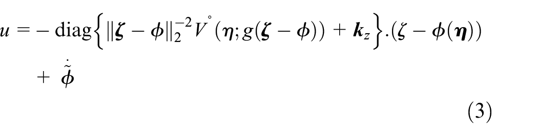
Control input

In the previous sections, our goal was to examine the stability of the system using the Lyapunov functions. In some cases, the Lyapunov functions can, in addition to stability, estimate the transient properties of the system or the structural uncertainties that are considered in the form of a slip in this paper. In particular, these functions allow us to estimate the convergence rate of linear or nonlinear systems.

In this section and previous sections, the definitions are given on differential inequalities. In the following, we show how using the Lyapunov analysis can be used to calculate the convergence rate of linear and nonlinear systems. In many control issues, the designer’s purpose is to select the appropriate control law for a particular system that leads to the stability and proper operation of the system under control.

Two methods are available for using Lyapunov direct method, both based on trial and error:

• I. In the first method, first, a form of hypothesized control rule, then we will find the Lyapunov function to prove the stability.

• II. In the second method, the first method assumes a candidate Lyapunov function and then a control rule, we will try to transform the candidate Lyapunov function into a real Lyapunov function for the controlled system by determining the appropriate control law.

In some nonlinear systems, systematic design procedures are developed based on two previous methods. Techniques such as sliding mode, ⁴¹ adaptive control method, ⁴² and physical design based approach ⁴³ are seen.

• Remark 8. As a nonlinear system may be stable asymptotic, but linear, it is only stable marginal, a nonlinear system may also be controllable, but its linear system is invulnerable.

• Theorem 5 . Consider the system:

$$\stackrel{·}{\eta }=\mathit{f}\left(\mathbf{\eta }\right)+\mathit{g}\left(\mathbf{\eta }\right)\mathbf{\zeta }$$

(1a)

that

$$\stackrel{·}{\mathbf{\zeta }}=\mathit{u}$$

(1b)

where $\mathbf{\eta }\in {\mathbb{R}}^n,\mathit{\zeta }\in {\mathbb{R}}^m$ . Assume that the subsystem (6a) can be stabilized by a control law $\mathbf{\zeta }=\varphi \left(\mathbf{\eta }\right)$ with $\varphi \left(0\right)=0$ , and that there is a regular (possibly nonsmooth) locally Lipschitz Lyapunov function $V\left(\mathbf{\eta }\right)$ for which there exists a positive definite, class ${\kappa }_{\infty }$ function $W\left(\eta \right)$ satisfying:

$$0<W\left(\mathbf{\eta }\right)⩽d,\forall d\in \mathit{D}$$

(2)

where $D\triangleq -{{{\displaystyle \cap }}^{\text{}}}_{\lambda \in \partial V\left(\eta \right)}{\lambda }^{T}F\left(f\left(\eta \right)+g\left(\eta \right)\varphi \left(\eta \right)\right)$ , and $\mathit{F}\left(h\left(x\right)\right)$ is the Filippov set of $\stackrel{·}{x}=h\left(x\right)$ . Then the following law asymptotically stabilizes (6):

$$\begin{array}{cc}\multicolumn{1}{c}{u=}& -\mathrm{diag}\{\Vert \mathbf{\zeta }-\varphi {\Vert }_2^{-2}{V}^{°}(\eta ;g(\mathbf{\zeta }-\varphi ))+{\mathit{k}}_z\}.(\zeta -\varphi \left(\mathbf{\eta }\right))\hfill \\ +\stackrel{.}{\stackrel{~}{\varphi }}\hfill \end{array}$$

(3)

where $V^{°}(.)$ is the generalized derivative, ⁴² $\stackrel{.}{\stackrel{~}{\varphi }}$ is the generalized time derivative, ² and ${\mathit{k}}_z$ , a positive constant gain vector, stabilizes asymptotically the system (6a)–(6b) to the origin.

Proof. Change of variables from ³⁶ :

$$\begin{array}{c}z=\mathbf{\zeta }-\varphi \left(\mathbf{\eta }\right)\hfill \\ \multicolumn{1}{c}{(6\mathrm{a})\mathrm{-}(6\mathrm{b})}& \stackrel{·}{\eta }=f\left(\mathbf{\eta }\right)+g\left(\mathbf{\eta }\right)\varphi \left(\mathbf{\eta }\right)+g\left(\mathbf{\eta }\right)z\hfill \\ \stackrel{·}{z}=\mathit{u}-\stackrel{·}{\varphi }\hfill \end{array}$$

taking

$$\mathit{v}=\mathit{u}-\stackrel{·}{\varphi }\Rightarrow \stackrel{·}{z}=\mathit{v}$$

consider Lyapunov function:

$$V_a(\mathbf{\eta },\mathbf{\zeta })\stackrel{\Delta }{=}V\left(\mathbf{\eta }\right)+\frac{1}{2}{z}^{T}z$$

derivative is

$${\stackrel{·}{\stackrel{~}{V}}}_a\stackrel{\Delta }{=}-W\left(\mathbf{\eta }\right)+{\cap }_{\lambda \in \partial \mathit{V}\left(\mathbf{\eta }\right)}{\lambda }^{T}g\left(\mathbf{\eta }\right)z+\frac{1}{2}{z}^T\mathit{v}$$

$\mathit{v}$ defined as

$$u=-\mathrm{diag}\{\Vert z{\Vert }_2^{-2}{V}^{°}(\eta ;g\left(\mathbf{\eta }\right)z)+{\mathit{k}}_z\}.(\zeta -\varphi \left(\mathbf{\eta }\right))z$$

definition of generalized derivative

$${\cap }_{\lambda \in \partial \mathit{V}\left(\mathbf{\eta }\right)}{\lambda }^{T}g\left(\mathbf{\eta }\right)z-V^{°}(\eta ;g\left(\mathbf{\eta }\right)z)⩽0$$

and ${\stackrel{·}{\stackrel{~}{V}}}_a$ becomes negative definite.

Theorem 6 at the point of discontinuity states that the control inputs are no longer a vector, but instead a set is defined by the definitions that any value in that set of values is acceptable, which means that the system is stable.

Applications

Problem description

In this section, as in Figure 1, along with the necessary basic parameters, the generalized coordinates for the tractor trailer system are $q={({\mathrm{x}}_{\mathrm{n}},{\mathrm{y}}_{\mathrm{n}},{\theta }_0,{\theta }_1\cdots {\theta }_{\mathrm{n}})}^{\mathrm{T}}$ , the values of control inputs $(u_i,{\omega }_i),(i=0,1,\dots ,N)$ , the links between the tractor links to the trailer as well as the trailer to the trailer $({\mathrm{P}}_1,{\mathrm{P}}_2,\cdots {\mathrm{P}}_{\mathrm{N}})$ , as well as the length of the $L_i$ links and the length of the $L_{\mathrm{hi}}$ inactive connections. Which show an N trailer wheel mobile robot for application in the use of the Lyapunov stability cases mentioned in previous sections? It should be noted that the connection of the trailers to the tractor driven by the inactive pins and off-axle. This type of connection is useful for causing the algebraic relationship between the control inputs, which can easily be accessed through the inputs of the $N$ trailer or the tractor. So here is the main purpose of controlling the last trailer, since a tractor with inactive (off-axle) trailer during rotation creates a problem as a jack-knife phenomenon in controlling the movement of the system, which can be replaced by the $N+3$ trailer’s generalized coordinates of the same trailer By reducing $N$ to the degree of system release associated with the angles generated by the link, the connections are the same as the coordinates of a non-trailer wheeled robot with the coordinates $q={({\mathrm{x}}_{\mathrm{n}},{\mathrm{y}}_{\mathrm{n}},{\theta }_{\mathrm{n}})}^{\mathrm{T}}$ for designing the input controllers of the system last trailer, and by connecting Listed between inputs in the further inputs of the tractor or trailer before $N_{i-1},(i=1,2,\dots ,n-1)$ . This is because of the inactive trailer used by the tractor using a physical off axle link solely for the equilibrium, which moves to the tractor but requires control of the trailer itself and trajectory the trailer by the trailer itself.

Figure 1.

Differentially driven wheeled mobile robot with N trailer.

The kinematic model a two-wheeled differential drive mobile robot with assuming the slip of actions in the control inputs as uncertainties in order to estimate the sudden disturbances entered into the structure of the system is given as:

$${\stackrel{·}{x}}_i=(u_i+{\delta }_{1i})\cos {\theta }_{\mathrm{i}},{\stackrel{·}{y}}_i=(u_i+{\delta }_{1i})\sin {\theta }_{\mathrm{i}},{\stackrel{·}{\theta }}_i={\omega }_i+{\delta }_{2i}$$

(4)

where ${\delta }_1$ , ${\delta }_2$ express a slip in direction of linear velocity and rotational velocity, respectively.

And dynamic equations of the mobile robot:

$$\{\begin{array}{c}\stackrel{·}{q}=G{\mathrm{v}}_i\hfill \\ \multicolumn{1}{c}{\left[\begin{array}{c}{\stackrel{·}{u}}_i\hfill \\ \multicolumn{1}{c}{{\stackrel{·}{\omega }}_i}\end{array}\right]=M{(x_i,y_i,{\theta }_i)}^{-1}(f-R(x_i,y_i,{\theta }_i,u_i,{\omega }_i))}\end{array}$$

(5)

$M$ is the inertia matrix of the system, ${\mathrm{v}}_i={({\omega }_i,u_i)}^T\mathrm{control}\mathrm{inputs}$ , $R$ is term containing Coriolis and centrifugal terms, and $f$ is the vector of input forces. To select $f$ , we select the $f=R(q_i,{\mathrm{v}}_i)+M\left(q_i\right)w$ term to create a control entry law, such as w, using the feedback law-making method.

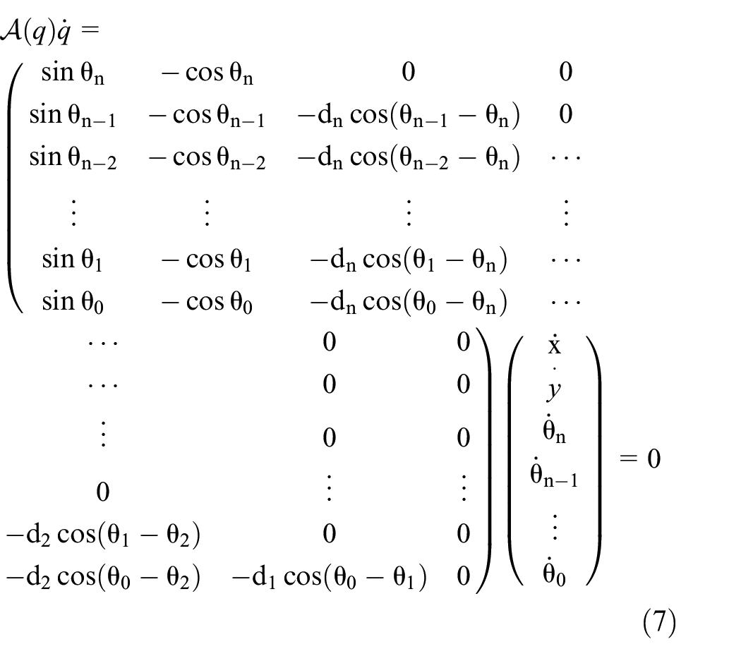
The kinematic robot is defined as for N trailer $\stackrel{·}{q}=\mathcal{S}\left(q\right){\mathrm{v}}_{\mathrm{i}}$ that $\mathcal{S}\left(q\right)$ is the natural orthogonal complement of constraint matrix, which is specified for the N trailer.

$$\mathcal{S}\left(q\right)=\left(\begin{array}{cc}\cos {\theta }_{\mathrm{n}}\hfill & 0\hfill \\ \multicolumn{1}{c}{\sin {\theta }_{\mathrm{n}}}& 0\hfill \\ \multicolumn{1}{c}{\frac{1}{{\mathrm{d}}_{\mathrm{n}}}\tan ({\theta }_{\mathrm{n}-1}-{\theta }_{\mathrm{n}})}& 0\hfill \\ \multicolumn{1}{c}{\frac{1}{{\mathrm{d}}_{\mathrm{n}-1}}\frac{\tan ({\theta }_{\mathrm{n}-2}-{\theta }_{\mathrm{n}-1})}{\cos ({\theta }_{\mathrm{n}-1}-{\theta }_{\mathrm{n}})}}& 0\hfill \\ \multicolumn{1}{c}{\frac{1}{{\mathrm{d}}_{\mathrm{n}-2}}\frac{\tan ({\theta }_{\mathrm{n}-3}-{\theta }_{\mathrm{n}-2})}{\cos ({\theta }_{\mathrm{n}-2}-{\theta }_{\mathrm{n}-1})\cos ({\theta }_{\mathrm{n}-1}-{\theta }_{\mathrm{n}})}}& 0\hfill \\ \multicolumn{1}{c}{⋮}& ⋮\hfill \\ \multicolumn{1}{c}{\frac{1}{{\mathrm{d}}_{\mathrm{n}-\mathrm{k}}}\frac{\tan ({\theta }_{\mathrm{n}-\mathrm{k}-1}-{\theta }_{\mathrm{n}-\mathrm{k}})}{\underset{\mathrm{i}=\mathrm{n}-\mathrm{k}}{\overset{\mathrm{n}-1}{\Pi }}\cos ({\theta }_{\mathrm{i}}-{\theta }_{\mathrm{i}+1})}}& 0\hfill \\ \multicolumn{1}{c}{⋮}& ⋮\hfill \\ \multicolumn{1}{c}{\frac{1}{{\mathrm{d}}_1}\frac{\tan ({\theta }_0-{\theta }_1)}{\underset{\mathrm{i}=1}{\overset{\mathrm{n}-1}{\Pi }}\cos ({\theta }_{\mathrm{i}}-{\theta }_{\mathrm{i}+1})}}& 0\hfill \\ \multicolumn{1}{c}{0}& 1\hfill \end{array}\right)$$

(6)

Also, the condition of limiting non-holonomic constraints must be the matrix equation ${\mathcal{S}}^{\mathrm{T}}\left(q\right){\mathcal{A}}^{\mathrm{T}}\left(q\right)=0$ , which can eventually be written for the trailer $N$ trailer:

$$\begin{array}{c}\mathcal{A}\left(q\right)\stackrel{·}{q}=\hfill \\ (\begin{array}{cccc}\sin {\theta }_{\mathrm{n}}\hfill & -\cos {\theta }_{\mathrm{n}}\hfill & 0\hfill & 0\hfill \\ \multicolumn{1}{c}{\sin {\theta }_{\mathrm{n}-1}}& -\cos {\theta }_{\mathrm{n}-1}\hfill & -{\mathrm{d}}_{\mathrm{n}}\cos ({\theta }_{\mathrm{n}-1}-{\theta }_{\mathrm{n}})\hfill & 0\hfill \\ \multicolumn{1}{c}{\sin {\theta }_{\mathrm{n}-2}}& -\cos {\theta }_{\mathrm{n}-2}\hfill & -{\mathrm{d}}_{\mathrm{n}}\cos ({\theta }_{\mathrm{n}-2}-{\theta }_{\mathrm{n}})\hfill & \cdots \hfill \\ \multicolumn{1}{c}{⋮}& ⋮\hfill & ⋮\hfill & ⋮\hfill \\ \multicolumn{1}{c}{\sin {\theta }_1}& -\cos {\theta }_1\hfill & -{\mathrm{d}}_{\mathrm{n}}\cos ({\theta }_1-{\theta }_{\mathrm{n}})\hfill & \cdots \hfill \\ \multicolumn{1}{c}{\sin {\theta }_0}& -\cos {\theta }_0\hfill & -{\mathrm{d}}_{\mathrm{n}}\cos ({\theta }_0-{\theta }_{\mathrm{n}})\hfill & \cdots \hfill \end{array}\hfill \\ \begin{array}{ccc}\cdots \hfill & 0\hfill & 0\hfill \\ \multicolumn{1}{c}{\cdots }& 0\hfill & 0\hfill \\ \multicolumn{1}{c}{⋮}& 0\hfill & 0\hfill \\ \multicolumn{1}{c}{0}& ⋮\hfill & ⋮\hfill \\ \multicolumn{1}{c}{-{\mathrm{d}}_2\cos ({\theta }_1-{\theta }_2)}& 0\hfill & 0\hfill \\ \multicolumn{1}{c}{-{\mathrm{d}}_2\cos ({\theta }_0-{\theta }_2)}& -{\mathrm{d}}_1\cos ({\theta }_0-{\theta }_1)\hfill & 0\hfill \end{array})\left(\begin{array}{c}\stackrel{·}{\mathrm{x}}\hfill \\ \multicolumn{1}{c}{\stackrel{.}{\begin{array}{c}y\hfill \\ \multicolumn{1}{c}{{\stackrel{·}{\theta }}_{\mathrm{n}}}\end{array}}}\\ \multicolumn{1}{c}{{\stackrel{·}{\theta }}_{\mathrm{n}-1}}\\ \multicolumn{1}{c}{⋮}\\ \multicolumn{1}{c}{{\stackrel{·}{\theta }}_0}\end{array}\right)=0\hfill \end{array}$$

(7)

Discontinuous kinematic control

Using Definitions 1 and 2 and Theorem 1 as outlined in the previous sections, we design the control input rule as follows for last trailer:

$$u_i=\mathrm{sgn}\left(x\right)k_u[(y_i^2-x_i^2)\cos {\theta }_i-2x_i{y}_i\sin {\theta }_i]$$

(8a)

$${\omega }_i=k_{\omega }(\arctan 2(2x_i{y}_i,x_i^2-y_i^2)-{\theta }_i)$$

(8b)

where $k_u$ and $k_{\omega }$ positive constants, and definition sign function:

$$\mathrm{sgn}\left(x\right)=\{\begin{array}{c}1x⩾0\hfill \\ \multicolumn{1}{c}{0x<0}\end{array}$$

(9)

Proof. Consider the positive semidefinite Lyapunov function. ⁴²

$$V_1(x,y)={\mathrm{e}}^{\frac{x_i}{x_i^2+y_i^2}}$$

(10a)

This function is defined everywhere. The function $V_1$ is defined for $(x_i,y_i,{\theta }_i)\in M^1=\{(x_i,y_i,{\theta }_i)|x⩾0\backslash \left\{0\right\}\}$ and

$$V_2(x,y)={\mathrm{e}}^{\frac{-x_i}{x_i^2+y_i^2}}$$

(10b)

for $(x_i,y_i,{\theta }_i)\in M^2=\{(x_i,y_i,{\theta }_i)|x<0\}.$ Note that $\{(x_i,y_i,{\theta }_i)|x=0\}\notin M^1,{\mathit{M}}^2$ and thus $V_1$ , $V_2$ are well defined. Then on each region $M^1,{\mathit{M}}^2$ , (10a) under control law (8) is asymptotically stable. In $M^1\backslash \{(x_i,y_i,{\theta }_i)|x=0\}:$

$${\stackrel{·}{V}}_1(x,y)=\frac{u_i{\mathrm{e}}^{\frac{x_i}{x_i^2+y_i^2}}}{{(x_i^2+y_i^2)}^2}[(y_i^2-x_i^2)\cos {\theta }_i-2x_i{y}_i\sin {\theta }_i]$$

(11a)

Similarly, in $M^2\backslash \{(x_i,y_i,{\theta }_i)|x=0\}$

$${\stackrel{·}{V}}_2(x,y)=\frac{-u_i{\mathrm{e}}^{\frac{-x_i}{x_i^2+y_i^2}}}{{(x_i^2+y_i^2)}^2}[(x_i^2-y_i^2)\cos {\theta }_i+2x_i{y}_i\sin {\theta }_i]$$

(11b)

Replace equation (13a) in (16):

$${\stackrel{·}{V}}_1={\stackrel{·}{V}}_2=\frac{-u_i{\mathrm{e}}^{\frac{-x_i}{x_i^2+y_i^2}}}{{(x_i^2+y_i^2)}^2}{[(x_i^2-y_i^2)\cos {\theta }_i+2x_i{y}_i\sin {\theta }_i]}^2⩽0$$

(12)

• Theorem 6. ² For $x=0$ , condition $\zeta ⩽0,\forall \zeta \in \stackrel{·}{\stackrel{~}{V}}$ is trivially satisfied. The set $\mathit{S}\stackrel{\Delta }{=}\{(x_i,y_i,{\theta }_i)|0\in \stackrel{·}{\stackrel{~}{V}}\}$ is given as $\mathit{S}\stackrel{\Delta }{=}\left\{(x_i,y_i,{\theta }_i)|x((y_i^2-x_i^2)\cos {\theta }_i-2x_i{y}_i\sin {\theta }_i)\right\}\mathrm{for}$ ${\stackrel{·}{V}}_1\mathrm{or}{\stackrel{·}{V}}_2\mathit{S}\stackrel{\Delta }{=}\left\{(x_i,y_i,{\theta }_i)|x((x_i^2-y_i^2)\cos {\theta }_i+2x_i{y}_i\sin {\theta }_i)\right\}.$

Which one to consider is not the same. And the result will be the same. In any point where $(y_i^2-x_i^2)\cos {\theta }_i-2x_i{y}_i\sin {\theta }_i=0$ , it is $|\arctan 2(2x_i{y}_i,x_i^2-y_i^2)-{\theta }_i|=\frac{\pi }{2}$

which means that ${\omega }_i=0$ . Thus, $\mathit{S}=\{(x_i,y_i,{\theta }_i)|x=0\}$ In $\mathit{S}$ we have: $u_i=k_u{y_i}^2\cos {\theta }_i,{\omega }_i=k_{\omega }(\arctan 2(0,-{y_i}^2)-{\theta }_i).$ For the invariant set $\mathit{E}\subset \mathit{S}$ , $y_i={\theta }_i=0$ , and so it is $\mathit{E}\equiv \left\{0\right\}.$ That ³⁵ f be Lipschitz near $x$ , ${\mathbf{\Omega }}_f$ the set of points where $f$ is non differentiable, and $\mathit{S}$ any set of Lebesgue measure zero in ${\mathbb{R}}^n$ .

In ${\stackrel{·}{V}}_1,{\stackrel{·}{V}}_2$ is satisfied for $(x,y)=(0,0)$ for all ${\theta }_i$ . For any invariant set in $(0,0,{\theta }_i)$ it should be:

$${\omega }_i=0\to {\theta }_i=0$$

(13)

by definition of arctan2. So system is asymptotically stable in set $M^1,{\mathit{M}}^2.$

• Lemma 1. ⁶ $M^1,M^2$ be two open connected subsets of ${\mathbb{R}}^n$ such that $M^1{{\displaystyle \cup }}^{\text{}}{M}^2={ℝ}^n\backslash \left\{0\right\}$  . Let $f^i:M^i\to {\mathbb{R}}^n,i=1,2$ be two vector fields. Assume also, that there exists a separating hypersurface $\Gamma$ with $0\in \Gamma$ and $\backslash \left\{0\right\}\subset M^1{{\displaystyle \cap }}^{\text{}}{M}^2$ . Let $C^i,C^2$ be two connected components of ${\mathbb{R}}^n\backslash \Gamma$ and assume that $C^i\subset M^i$ and that $f^i$ points toward $C^i$ on $\Gamma$ for $i=1,2$ . Finally assume that $f^1$ , $f^2$ are asymptotically stable on $M^1,M^2$ . Then, the vector field $f:{\mathbb{R}}^n\to {\mathbb{R}}^n$ defined by

$$f=\{\begin{array}{cc}{f}^1\left(x\right)& ifx\in \left(\Gamma \backslash \left\{0\right\}{{\displaystyle \cup }}^{\text{}}{C}^1\right)\\ f^2\left(x\right)& ifx\in C^2\\ 0& ifx=0\end{array}$$

is globally asymptotically stable.

• Remark 9. Desired convergence of ${\theta }_i$ to ${\theta }_{\mathrm{id}}$ we select the control input below:

$${\omega }_i=k_{\omega }(\arctan 2(2x_i{y}_i,x_i^2-y_i^2)-{\theta }_i)$$

$$+\frac{2u_i(x_i\sin {\theta }_i-y_i\cos {\theta }_i)}{x_i^2+y_i^2}$$

which implies that

$${\stackrel{·}{\theta }}_i-{\stackrel{·}{\theta }}_{\mathrm{id}}=-k_{\omega }({\theta }_i-{\theta }_{\mathrm{id}})$$

if

$$E={\theta }_i-{\theta }_{\mathrm{id}}\Rightarrow \stackrel{·}{E}+k_{\omega }E=0$$

which leads to the creation of a stable equation whose convergence is guaranteed.

Consider Lyapunov direct method of Theorem 7:

• Theorem 7. ² Let $\stackrel{·}{x}=f(x,t)$ be essentially locally bounded and $0\in \mathit{K}\left[\mathit{f}\right](0,t)$ in a region $Q¹\{x\in {\mathbb{R}}^n|x<r\}\times \{t|t_0⩽t<\infty \}$ . Also, let $V:{\mathbb{R}}^n\times \mathbb{R}\to \mathbb{R}$ be a regular function satisfying

$$V(0,t)=0$$

and

$$0<V_1\left(x\right)⩽V(x,t)⩽V_2\left(x\right),\mathrm{for}\mathrm{x}\ne 0$$

in Q for some $V_1$ , $V_2\in \mathcal{K}.$

• (1)  $\stackrel{·}{\stackrel{~}{\mathit{V}}}⩽0$ in Q implies $\mathit{x}\equiv 0$ is a uniformly stable solution.

• (2) If in addition, there exists a class $\mathcal{K}$ function $\mathit{w}(.)$ in Q with the property

$$\stackrel{·}{\stackrel{~}{V}}(x,t)⩽w\left(x\right)<0$$

then the solution $x\left(t\right)\equiv 0$ is uniformly asymptotically stable.

Feedback control law

A general formula can be used for virtual inputs of both sections of a tractor attached to a trailer or two trailer backward trains for $i=1...,N$ wrote:

$${\mathrm{v}}_i=J_i\left({\theta }_{\mathrm{i}}\right){\mathrm{v}}_{i-1}$$

(14)

Where

$$J_i\left({\beta }_{\mathrm{i}}\right)=\left[\begin{array}{cc}-\frac{L_{\mathrm{hi}}}{L_i}\cos {\beta }_{\mathrm{i}}\hfill & \frac{1}{L_i}\sin {\beta }_{\mathrm{i}}\hfill \\ \multicolumn{1}{c}{L_{\mathrm{hi}}\sin {\beta }_{\mathrm{i}}}& \cos {\beta }_{\mathrm{i}}\hfill \end{array}\right]$$

(15)

is the transformation matrix with the inverse

$$J_i^{-1}\left({\beta }_{\mathrm{i}}\right)=\left[\begin{array}{cc}-\frac{L_i}{L_{\mathrm{hi}}}\cos {\beta }_{\mathrm{i}}\hfill & \frac{1}{L_{\mathrm{hi}}}\sin {\beta }_{\mathrm{i}}\hfill \\ \multicolumn{1}{c}{L_i\sin {\beta }_{\mathrm{i}}}& \cos {\beta }_{\mathrm{i}}\hfill \end{array}\right]$$

(16)

the result of the matrix determination is $\det \left(J_i\left({\beta }_{\mathrm{i}}\right)\right)=-\frac{L_{\mathrm{hi}}}{L_i}$ , which is necessary for reversibility $L_i\ne 0$ .

inverse relation to (3) can be written as

$${\mathrm{v}}_{i-1}=J_i^{-1}\left({\beta }_{\mathrm{i}}\right){\mathrm{v}}_i$$

(17)

Equations (14) and (17) make it possible to sum up the sum of the nth trailer attached to the tractor, which has the task of conducting along the vehicle chain.

$${\text{v}}_i={\displaystyle \prod }_{j=i}^1{J}_i\left({\text{β}}_{\text{i}}\right){\text{v}}_0,i=1,\dots ,N$$

(18)

but if we start with the tractor input equations and get the connection between the inputs of the last tractor, then the relation must be changed by equation (18).

$${\mathrm{v}}_{i-1}=\underset{j=i}{\overset{N}{\Pi }}{J}_i^{-1}\left({\beta }_{\mathrm{i}}\right){\mathrm{v}}_i,i=1,\dots ,N$$

(19)

$${\beta }_{\mathrm{i}}={\theta }_{\mathrm{i}-1}-{\theta }_{\mathrm{i}}$$

(20)

From the derivative of the connecting angle

$${\stackrel{·}{\beta }}_{\mathrm{i}}={\omega }_{\mathrm{i}-1}-{\omega }_{\mathrm{i}}$$

(21)

Using combining equations (4), (5), and (20) for kinematic $\stackrel{·}{q}=\mathcal{S}\left(q\right){\mathrm{v}}_0$ connecting angle a general formula can be obtained without the need to calculate the single-link connection between the inputs. The C index is the connection sign.

$$\left[\begin{array}{c}{\stackrel{·}{\beta }}_1\hfill \\ \multicolumn{1}{c}{{\stackrel{·}{\beta }}_2}\\ \multicolumn{1}{c}{⋮}\\ \multicolumn{1}{c}{{\stackrel{·}{\beta }}_{\mathrm{i}}}\\ \multicolumn{1}{c}{⋮}\\ \multicolumn{1}{c}{{\stackrel{·}{\beta }}_{\mathrm{N}}}\\ \multicolumn{1}{c}{{\stackrel{·}{\mathrm{x}}}_{\mathrm{n}}}\\ \multicolumn{1}{c}{{\stackrel{·}{\mathrm{y}}}_{\mathrm{n}}}\\ \multicolumn{1}{c}{{\stackrel{·}{\theta }}_{\begin{array}{c}\mathrm{N}\hfill \\ \multicolumn{1}{c}{..}\end{array}}}\end{array}\right]=\left[\begin{array}{c}{\mathrm{c}}^{\mathrm{T}}(\mathrm{I}-{\mathrm{J}}_1\left({\beta }_1\right))\hfill \\ \multicolumn{1}{c}{{\mathrm{c}}^{\mathrm{T}}(\mathrm{I}-{\mathrm{J}}_2\left({\beta }_2\right)){\mathrm{J}}_1\left({\beta }_1\right)}\\ \multicolumn{1}{c}{⋮}\\ \multicolumn{1}{c}{{\mathrm{c}}^{\mathrm{T}}(\mathrm{I}-{\mathrm{J}}_{\mathrm{i}}\left({\beta }_{\mathrm{i}}\right))\underset{\mathrm{j}=\mathrm{i}-1}{\overset{1}{\Pi }}{\mathrm{J}}_{\mathrm{j}}\left({\beta }_{\mathrm{j}}\right)}\\ \multicolumn{1}{c}{⋮}\\ \multicolumn{1}{c}{{\mathrm{c}}^{\mathrm{T}}(\mathrm{I}-{\mathrm{J}}_{\mathrm{N}}\left({\beta }_{\mathrm{N}}\right))\underset{\mathrm{j}=\mathrm{N}-1}{\overset{1}{\Pi }}{\mathrm{J}}_{\mathrm{j}}\left({\beta }_{\mathrm{j}}\right)}\\ \multicolumn{1}{c}{{\mathrm{d}}^{\mathrm{T}}\underset{\mathrm{j}=\mathrm{N}}{\overset{1}{\Pi }}{\mathrm{J}}_{\mathrm{j}}\left({\beta }_{\mathrm{j}}\right)\cos {\theta }_{\mathrm{N}}}\\ \multicolumn{1}{c}{{\mathrm{d}}^{\mathrm{T}}\underset{\mathrm{j}=\mathrm{N}}{\overset{1}{\Pi }}{\mathrm{J}}_{\mathrm{j}}\left({\beta }_{\mathrm{j}}\right)\sin {\theta }_{\mathrm{N}}}\\ \multicolumn{1}{c}{{\mathrm{c}}^{\mathrm{T}}\underset{\mathrm{j}=\mathrm{N}}{\overset{1}{\Pi }}{\mathrm{J}}_{\mathrm{j}}\left({\beta }_{\mathrm{j}}\right)}\end{array}\right]v_0$$

(22)

${\mathrm{v}}_0={\left[\begin{array}{cc}{\omega }_0\hfill & u_0\hfill \end{array}\right]}^T$ is the control input of the tractor, in which ${\mathrm{c}}^{\mathrm{T}}=\left[10\right]$ , ${\mathrm{d}}^{\mathrm{T}}=\left[01\right]$ , and $I\in R^{2\times 2}$ is a one-dimensional matrix. In fact, the equation (22) for the summary of equations (4) and (14–21) in the analysis of the kinematic model for controller design method is presented in this paper.

Simulation result

Design of the controller for third trailer

For the last trailer we assume here is N=3 and the extraction of the governing equations of the problem, the relationship between the input of the third trailer and the tractor, which is actually the aim of obtaining the linear velocity of the third trailer ${\omega }_0$ and the angular velocity of the tractor $u_3$ , which is the equation of the obtained relations This can be achieved. For simplicity, we will use the control workflows obtained in the previous step for the last trailer, assuming that the control inputs of the third trailer ( $u_{\mathrm{i}}$ = $u_3$ , ${\omega }_i$ = ${\omega }_3$ ) are used to reach the tractor control inputs. In fact, using the new solution as described following for the equation, the inactivity external linking (off axle) of the links at the pinpoint causes the control entries to be easily expressed in the form of a square matrix for linear velocity and rotational velocity. The advantage of this type of connection is that there is no longer a need for time-dependent (derived) equation between generalized coordinates, since in general the derivative also results in instability, complexity of the parameters, and the extension of the time of convergence.

$${\mathrm{v}}_3=\left[\begin{array}{c}{\omega }_3\hfill \\ \multicolumn{1}{c}{u_3}\end{array}\right]$$

(23)

That

$${\mathrm{v}}_3=\{\begin{array}{c}{\omega }_i=k_{\omega }(\arctan 2(2x_i{y}_i,x_i^2-y_i^2)-{\theta }_i)-{\delta }_{n2}\hfill \\ u_i=\mathrm{sgn}\left(x\right)k_u[(y_i^2-x_i^2)\cos {\theta }_i-2x_i{y}_i\sin {\theta }_i]-{\delta }_{n1}\hfill \end{array}$$

(24)

From equation (4), we can write off the equation of connection off axle to obtain ${\mathrm{v}}_2$ inputs:

$$\left[\begin{array}{c}{\omega }_2\hfill \\ \multicolumn{1}{c}{u_2}\end{array}\right]=\left[\begin{array}{cc}-\frac{L_3}{L_{h3}}\cos {\beta }_3\hfill & \frac{1}{L_{h3}}\sin {\beta }_3\hfill \\ \multicolumn{1}{c}{L_3\sin {\beta }_3}& \cos {\beta }_3\hfill \end{array}\right]\left[\begin{array}{c}{\omega }_3\hfill \\ \multicolumn{1}{c}{u_3}\end{array}\right]$$

(25)

Also for ${\mathrm{v}}_1$

$$\left[\begin{array}{c}{\omega }_1\hfill \\ \multicolumn{1}{c}{u_1}\end{array}\right]=\left[\begin{array}{cc}-\frac{L_2}{L_{h2}}\cos {\beta }_2\hfill & \frac{1}{L_{h2}}\sin {\beta }_2\hfill \\ \multicolumn{1}{c}{L_2\sin {\beta }_2}& \cos {\beta }_2\hfill \end{array}\right]\left[\begin{array}{c}{\omega }_2\hfill \\ \multicolumn{1}{c}{u_2}\end{array}\right]$$

(26)

And inputs tractor

$$\left[\begin{array}{c}{\omega }_0\hfill \\ \multicolumn{1}{c}{u_0}\end{array}\right]=\left[\begin{array}{cc}-\frac{L_1}{L_{h1}}\cos {\beta }_1\hfill & \frac{1}{L_{h1}}\sin {\beta }_1\hfill \\ \multicolumn{1}{c}{L_1\sin {\beta }_1}& \cos {\beta }_1\hfill \end{array}\right]\left[\begin{array}{c}{\omega }_1\hfill \\ \multicolumn{1}{c}{u_1}\end{array}\right]$$

(27)

For slip on other inputs, one can also consider the expressions of the multiplied factors in them, and finally, all the slip terms derived from ${\delta }_1$ and ${\delta }_2$ are taken into account and as a coefficient for them in equations next, this may slightly complicate the system equations or prolong the resolution time. The resulting is very different from that of the total input equations of each trailer and tractor part at the rotational input ${\delta }_2$ and at the input of the linear velocity ${\delta }_1$ in each step, we reduce the inputs at that stage, which makes it easier to solve the problem, without the result of that. The next section describes how to calculate these slip.

In summary, from equations (4) and (18), we can derive the relationship between the traverses of the third trailer with the tractor in summary form from the product of the following multiplication

$${\mathrm{v}}_3=J_1\left({\beta }_1\right)J_2\left({\beta }_2\right)J_3\left({\beta }_3\right){\mathrm{v}}_0\Rightarrow {\left(\begin{array}{cc}{\omega }_0\hfill & u_3\hfill \end{array}\right)}^T$$

(28)

In the simulations, the gains used are set as $k_u=10,k_{\omega }=3,k_{\mathrm{z}}=10$ , $L_{\mathrm{h}}=L_{\mathrm{h}1}=L_{\mathrm{h}2}=L_{\mathrm{h}3}=0.17$ , $L=L_1=L_2=L_3=0.05$ .

The control benefits are assumed to be positive values in order to satisfy the closed loop system. Therefore, in order to have good performance at the same time and reasonable control inputs, the control gain has been selected using the trial and error method and the simultaneous review of the function of the closed loop system and the amount of control inputs. Therefore, it is expected that, starting with different initial conditions and with limited time, the robot tracking errors are convergent around zero and the transient responses of the system are eliminated, and the robot follows the reference path directions.

Slip estimation

A system that provides attachment information on the status of the current state of the process and in order to identify the process. Then, the performance of the current system is compared with the desired or optimal state and based on which decision is made to adapt the system. Finally, the correction is applied to the system in order to reach the desired state. Therefore, there will be three methods of identifying, deciding, and correcting in a comparative system. Achieving high performance in control systems, when the dynamic characteristics of the controlled process are largely uncertain. When these characteristics change over and over again during system operation. The idea is to design a controller that can be adapted to change the process dynamics and disturbance characteristics. The processes of an adaptive system include three steps. The first step is to identify unknown parameters, such as adding slip to the system or measuring an index of performance (IP). The next step is to decide on the control method used to design the controller, which uses the method of stability of the Lyapunov function in this problem. In the final stage, the correction of the parameters of the controller or the input signal with a conformable law is to eliminate the error and converge all the paths to the reference point. In Figure 5, these steps are also shown as related equation and related signals in the blocks. One can summarize the schematic generalizations of the adaptive controller scheme in three general ways to be defined:

• (a) The design of the control loop that controls the function of the closed loop system relative to the variations of the parameters of the main system model is insensitive. That (sensitivity) will be responsive only in a small range of parameter variations.

• (b) Measurement of immediateparameters of the system model and correction of the parameters of the control law in terms of it. (The impossibility of measuring some of the parameters or, at the very least, the impossibility of measuring and determining the immediate moment.)

• (c) Comparison of the immediate indicators of the actual performance of the control system with desirable indicators and the revision of the control of the feedback based on the observed difference between the two.

To estimate the slip in the following way

$$\left(\begin{array}{c}{\stackrel{·}{x}}_3\hfill \\ \multicolumn{1}{c}{{\stackrel{·}{y}}_3}\\ \multicolumn{1}{c}{{\stackrel{·}{\omega }}_3}\end{array}\right)=\left(\begin{array}{cc}\cos {\theta }_3\hfill & 0\hfill \\ \multicolumn{1}{c}{\sin {\theta }_3}& 0\hfill \\ \multicolumn{1}{c}{0}& 1\hfill \end{array}\right)\left(\begin{array}{c}{u}_3+{\delta }_1\hfill \\ \multicolumn{1}{c}{{\omega }_3+{\delta }_2}\end{array}\right)$$

(29)

The main purpose of slip estimation is to use the method described in this system, or in general, linear, and nonlinear systems, to approximate or adaptive as much as possible the performance indicators of the ring system depending on the desired parameters in the presence of uncertainty and the existence of changes in the model and operating conditions of the system. Describes the optimal behavior of the closed loop system and determines the appropriate control law with adjustable geometric and control parameters. The results of the following are indicative of the slip estimation and designed controller. ⁴⁴

In general, in many control issues, especially in non-holonomic systems such as a WMR with an N-trailer in this paper, the following factors are considered in the kinematics of the problem of retrofitting and estimating slip from a new method that is described below for the problem:

• (d) Change in process conversion function, and uncertainty of initial values and change of system coefficients

• (e) Disturbance

• (f) Changing the input profile and structure

• (g) Nonlinear operation in complex systems

• (h) Unknown process parameters are selected when the control system is selected for a new process

Slip estimation

To estimate the slips (uncertainties) applying to the kinematic system of wheeled mobile robot with $N$ trailer, we can assume that the variables of the state $q={(\mathrm{x}\mathrm{y}{\theta }_{\mathrm{n}}{\theta }_{\mathrm{n}-1}\dots {\theta }_0)}^{\mathrm{T}}\in {\mathrm{R}}^{\mathrm{n}+3}$ can be measured with a specific time interval, such as $\mathcal{T}$ , using measuring sensors (e.g. a visual system) at a specified time, and steps taken before it is measured. With this assumption, the simplest method for estimating the slip values can be calculated from equation (32). In this regard, taking into account the kinematic equation of the system from equation (4), we can estimate the slip estimation vector ${\hat{\delta }}_n={\left({\hat{\delta }}_1{\hat{\delta }}_2\right)}^T$ in general for the $\mathrm{nth}$ space state of the system at $n$ and $n-1$ stages:

$$\begin{array}{c}{s}^{\#}={\left(s^T\left(q_i\right)s\left(q_i\right)\right)}^{-1}{s}^T\left(q_i\right)=\hfill \\ s^{\#}\left(\begin{array}{c}\stackrel{·}{\mathrm{x}}\left(\mathrm{k}\right)-u_1(k-1){\mathrm{C}}_{{\theta }_1(k-1)}\hfill \\ \multicolumn{1}{c}{\stackrel{·}{\mathrm{y}}\left(\mathrm{k}\right)-u_1(k-1){\mathrm{S}}_{{\theta }_1(k-1)}}\\ \multicolumn{1}{c}{\begin{array}{c}{\stackrel{·}{\theta }}_1\left(\mathrm{k}\right)-\frac{u_1(k-1)}{d}{\mathcal{T}}_{{\theta }_0(k-1)-{\theta }_1(k-1)}\hfill \\ \multicolumn{1}{c}{{\stackrel{·}{\theta }}_0\left(\mathrm{k}\right)-u_2(k-1)}\end{array}}\end{array}\right)\hfill \end{array}$$

(30)

$s^{\#}$ is used for square inversion when the square matrix $s\left(q_i\right)=\left(\begin{array}{cc}\cos {\theta }_{\mathrm{i}}\hfill & 0\hfill \\ \multicolumn{1}{c}{\sin {\theta }_{\mathrm{i}}}& 0\hfill \\ \multicolumn{1}{c}{0}& 1\hfill \end{array}\right)$ is not used.

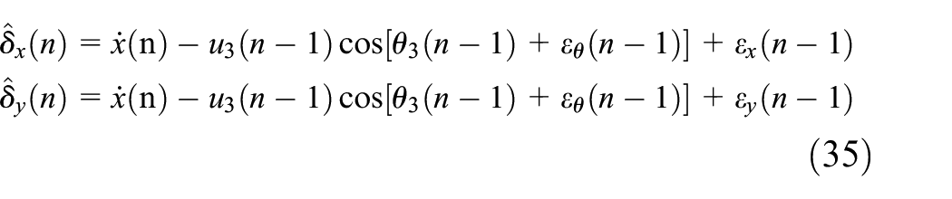
If we consider equation (36) for a trailer, then, in order to obtain the estimation of the slippage in the system $s\left(q_i\right)$ , we will account for equation (9), and for ${\stackrel{·}{q}}_i\left(t\right)-s\left(q_i\right)u_i$ :

$$\hat{\delta }=s^{\#}({\stackrel{·}{q}}_i\left(t\right)-s\left(q_{i-1}\right)u_i)$$

(31)

Slip estimates now can be used in equation (31) instead of the signals $({\delta }_1,{\delta }_2)$ obtained in the stability equations and control inputs, which are unknown in practice and their effect on intangible control of the system. ²⁹

Therefore, all the relations mentioned for stabilizing a tractor connected to several trailers can be seen by the back-stepping method and in the presence of sliding trailer wheels, the control process and obtaining control inputs by applying the adaptive rules obtained in the form of diagram (Figure 2).

Figure 2.

System control diagram for tractor with three trailers and joint connection transfer module.

The In the diagram in Figure 4, the controller receives the reference input and generates the input signal of the desired kinematic model. Due to the presence of slips, system variables are associated with uncertainties, and to compensate for these uncertainties and follow the reference path by the robot, modify the adaptive rules by estimating the slips at any time controlling proper control input leads the real robot to the reference robot to reduce the tracking error to zero. A signal is also input from the output of the control inputs to the function $J_1\left({\beta }_1\right)$ to convert the inputs from the trailer to the tractor inputs, which aims to connect the inputs of the last trailer using the structural equations of the connections via an external link (off-axis) is inactive.

Simulation of results

In this section, we will review and compare the results in this method. In this part, which is stabilization around a certain situation with the help of Lyapunov functions, to validate the relations and methods used in different initial conditions and with different angles, the path of the object is at any point and with any position of the last trailer of the robot, which is the same. The trailer is the third, and also with stabilization conditions with an angle of 45° in the presence of slip, without slip, active without slip estimator to compensate for errors and slips, as well as the system response in the presence of slip when there is without slip estimator to compensate for slip uncertainties.

The control inputs of the system inputs for stabilization are considered as $k_v=6.1$ and $k_w=1.8$ and the length of the tractor-trailer connection links in the external axle connection is $L_h=0.35$ and $L=2$ m. Regarding the proposed control parameters, it should be noted that the control gains in order to satisfy the stability of the closed loop system are assumed to be positive values. Therefore, in order to have proper performance and reasonable control inputs at the same time, control gains have been selected using trial and error method and simultaneous review of closed loop system performance and amount of control inputs. Since the stability of the problem in text relations has been proven, it is expected that starting from different initial conditions and over a limited time, the robot path errors will converge around zero or any desired point and the system transient responses will disappear, and the robot be at the desired point.

The considered slips are added to the system kinematics according to the following equation.

$${\delta }_n=\{\begin{array}{c}{\delta }_{31}=\{\begin{array}{c}0\mathrm{cte}\hfill \\ \multicolumn{1}{c}{1.60.05⩽t⩽0.2}\end{array}\hfill \\ \multicolumn{1}{c}{{\delta }_{32}=\{\begin{array}{c}0\mathrm{cte}\hfill \\ \multicolumn{1}{c}{1.60.05⩽t⩽0.2}\end{array}}\end{array}$$

(32)

And

$${\delta }_n=\{\begin{array}{c}{\delta }_{31}=\{\begin{array}{c}0\mathrm{cte}\hfill \\ \multicolumn{1}{c}{620⩽t⩽30}\end{array}\hfill \\ \multicolumn{1}{c}{{\delta }_{32}=\{\begin{array}{c}0\mathrm{cte}\hfill \\ \multicolumn{1}{c}{320⩽t⩽30}\end{array}}\end{array}$$

(33)

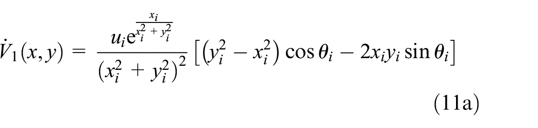
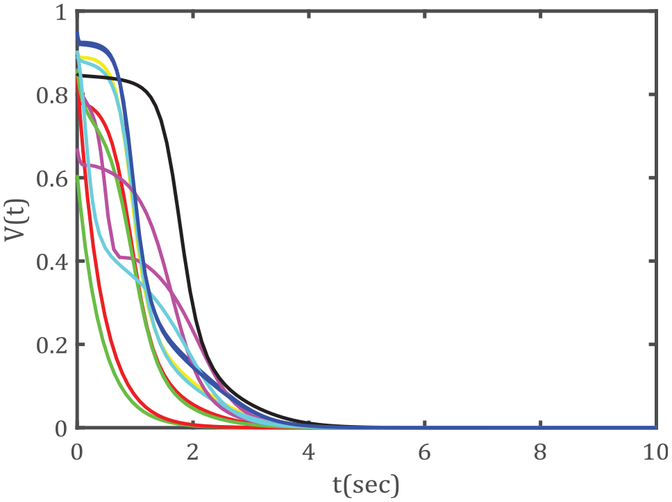
The Lyapunov function considered in equations (11a) and (11b) is three-dimensional to show certain positive values of the function considered as follows.

As can be seen in the figure above, all the values specified for the V function in Figure 3 are positive and definite, meaning that the selected Lyapunov function according to Lyapunov stability criteria has positive values in all x and y.

Figure 3.

Definite positive Lyapunov candidate function.

In the continuation of this discussion, the values of Lyapunov function for different initial conditions by applying slip in the presence and absence of the estimator in comparative cases can be seen in Figures 4 and 5.

Figure 4.

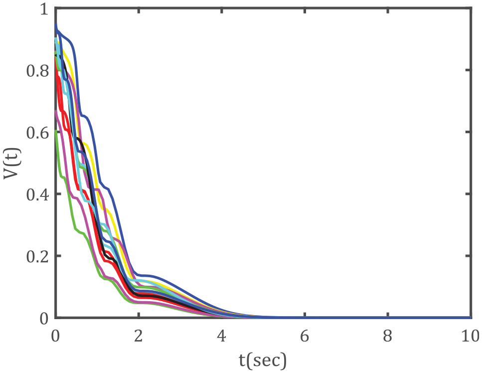
Time-history of Lyapunov function in the stabilization different initial conditions in the presence of slip (32) without estimator.

Figure 5.

Time-history of Lyapunov function in the stabilization different initial conditions in the presence of slip (32) with estimator.

In fact, in Figure 4 it can be seen that in the various initial conditions while the slip is applied to the system in the applied range, Lyapunov function as in Figure 5 has made an acceptable estimate of the slip but in Figure 4 the function Converged as a step function and impact function and as a steeper slope (broken functions) to compensate for slip, while in Figure 5 Lyapunov function with a soft shape and with a time delay less than Figure 4 and a function It has continuously converged the Lyapunov function with a smooth slope.

In Figures 6 and 7 the path of the robot in the tracking path to control and direct it to any desired point, here we have considered the point (0 and 0). From different initial conditions and angle zero and angle 45 for the last trailer (third) to the target point in the presence and absence of the slider estimator and the application of perturbations into the system is shown as slip.

Figure 6.

Time-history of Lyapunov function in the stabilization different initial conditions in the presence of slip (32) without estimator.

Figure 7.

Time-history of Lyapunov function in the stabilization different initial conditions in the presence of slip (32) without estimator.

In Figures 6 and 7 in both figures, with different initial conditions with different angles of the starting point of the trailer tractor, it can be inferred that even if a slip is applied to the system in both cases, either with a slip estimator or without the slider estimator, the system has converged to the desired target point, but with the difference that in the system without the slider, the trailer has deviated from the path to compensate for the slip, which has returned to the main path after these fluctuations. Has deviated from the path, which shows that the estimator, despite the application of slip (except in very large slips, which diverges the system in the non-estimator state, even in these cases, always brings the robot to the desired point) has little effect on tracking the path. The tractor does not leave trailers.

Figures 8 and 9 show the control inputs of the last trailer (third trailer) for different initial conditions in the presence of slips in the presence and absence of the estimator.

Figure 8.

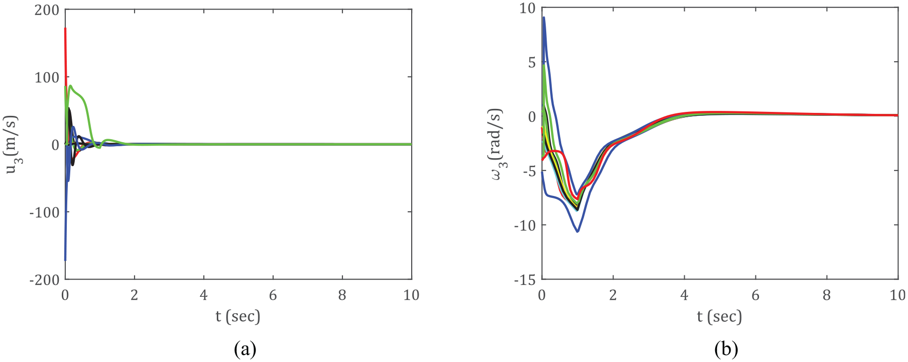
(a) Control linear input in different initial conditions in the presence of slip (32) without estimator and (b) control rotational input in different initial conditions in the presence of slip without estimator.

Figure 9.

(a) Control linear input in different initial conditions in the presence of slip (32) with estimator and (b) control rotational input in different initial conditions in the presence of slip with estimator.

In Figures 8 and 9, which show the linear and angular control inputs of the trailer tractor, respectively, the linear input has acted very strongly in estimating the slips and has converged the linear velocity of the robot. In the rotational speed of the robot due to the rotation of the trailer and the connected links, which itself creates complex conditions for stabilization and control of the system, and its control has discontinuous and nonlinear equations with linear velocity with a longer delay than the linear velocity of slip estimation. And put the robot at the right angle to be at the desired target point.

But as shown in Figure 8, the system without estimator shows better performance than the system in Figure 9 with the angular and linear velocity estimator than in Figure 8 because, as in the previous figures, the efficiency of the rules The adaptive proposed method for compensating and estimating the effects of slippage was approved. Figure 9 also shows that the adaptive rules designed in the problem are well able to compensate for the slip applied to the system.

Finally, the control errors for the target point by sliding and in the presence and absence of the estimator together in Figures 10 to 12 for the third trailer (last trailer) for the coordinates. The generalizations of the third trailer are compared.

Figure 10.

(a) Time-history of stabilization errors in the x direction for a three-trailer TTWR from different starting configurations, in the presence of slip without estimator. (b) Time-history of stabilization errors in the x direction for a three-trailer TTWR from different starting configurations in the presence of slip (32) with the estimator.

Figure 11.

(a) Time-history of stabilization errors in the y direction for a three-trailer TTWR from different starting configurations. In the presence of slip without estimator. (b) Time-history of stabilization errors in the y direction for a three-trailer TTWR from different starting configurations in the presence of slip (32) with the estimator.

Figure 12.

(a) Time-history of stabilization errors in the θ angle for a three-trailer TTWR from different starting configurations. In the presence of slip without estimator. (b) Time-history of stabilization errors in the θ angle for a three-trailer TTWR from different starting configurations in the presence of slip (32) with the estimator.

Figures 10 to 12 in Section a, which show the non-estimating slip compensation phenomenon for the proposed controller, show less controlling control signals and a smoother transient response. To evaluate the performance of the applied controller against slip, it shows that the method in question has been able to provide less chattering and compensation time for slips in less time in part b than part a in the figures.

The results show that the control algorithm based on Lyapunov function with slip estimator has a good performance in controlling the trajectory of the TTWM in following the path and converging the trailer system in the desired position and stabilizing the Lyapunov function with the algorithm in the presence of wheel slip shows itself. As can be seen, for different initial conditions, starting from different points, error signals in the presence and absence of slip with angles and different points in the range of slip application after a limited time, the wheeled robot reaches the desired point and the system error signal to It converges to zero and compensates for this phenomenon during the control of the system by applying slips, which indicates the proper design of control inputs designed with the help of adaptive rules that move the robot in any situation. Asymptotic stability converges.

Comparing results

To validate the model, we compare the results of this paper with the application of relation slip (33) with the reference results. ²⁹

Reference paths are considered in different ways and with the following equations:

$$\{\begin{array}{c}\multicolumn{1}{c}{{\mathrm{x}}_{\mathrm{r}}\left(t\right)=\left((\mathrm{R}+1)\cos \left(\frac{\mathrm{at}}{T}\right)\right)(\mathrm{C}+\cos \left(\frac{\mathrm{bt}}{T}\right))}\\ \multicolumn{1}{c}{{\mathrm{y}}_{\mathrm{r}}\left(t\right)=\left((\mathrm{R}+1)\cos \left(\frac{\mathrm{at}}{T}\right)\right)(\mathrm{C}+\sin \left(\frac{\mathrm{bt}}{T}\right))}\end{array}$$

(34)

Table 1 shows the values of the parameters required to plot the reference paths.

Table 1.

Path parameters.

Path	R	a	T	b	C
Path #1	4	36	50	4	0
Path #2	2	18	50	6	0

Figure 13 shows the upper boundary estimation of non-parametric uncertainties with the boundary estimation. And updates at any time, which is absolutely necessary to increase the control resistance and improves the system resistance in estimating the system uncertainties and does not deviate the trailer tractor from the target point or path.

Figure 13.

Control inputs in two compared stabilization methods with adaptive control.

Comparing the Lyapunov function in terms of time in Figure 14, it can be seen that the function considered in this paper is not changed due to the proposed Lyapunov backpacking function due to slipping in the specified range and the function Lyapunov converges in the zero neighborhood while the Lyapunov backstepping function fluctuates a lot and converges over a period of time over a longer period of time than the proposed function in a range. The observed changes show that the proposed system has converged the system without any time delay and in the fastest possible time due to moment-by-moment estimation and elimination of these uncertainties, but in the backstepping method the system fluctuates and a time delay is much more than Lyapunov function. Converges, indicating the high efficiency of the proposed method in resolving the uncertainties entered in the system.

Figure 14.

Time-history of Lyapunov function stabilization and adaptive backstepping in the presence of slip.

As can be seen from Figure 15, the proposed controller performance for stabilizing the system state variables in both methods shows that it is softer and smoother than the controller performance (adaptive backstepping). The simulations show that as the initial tracking error for both controllers increases, the controller control signals (adaptive backstepping) become rougher and a transient tracking response is obtained more unevenly. While the proposed controller shows less controlling signals and a smoother transient response. To evaluate the performance of the controller against the applied slip, it shows that the method in question has been able to provide less chattering and compensation time for slips in less time than the comparative method. Figure 15 and sections (a -c) actually show the state variables of the wheeled robot system, so that in Figure (a) the variable x1 has the same temporal variations of the generalized coordinates in the longitudinal direction, i.e. x, for both the proposed and comparative methods of the paper. Indicates in system mode space control. Also, for section (b), the diagram describes the temporal changes in the transverse direction, i.e. the lateral speed y, and at the end, the section shows the angular changes of the trailer tractor, which changes and controls the system mode variables in the proposed controller compared to the backstepping controller experience smoother and converge faster.

Figure 15.

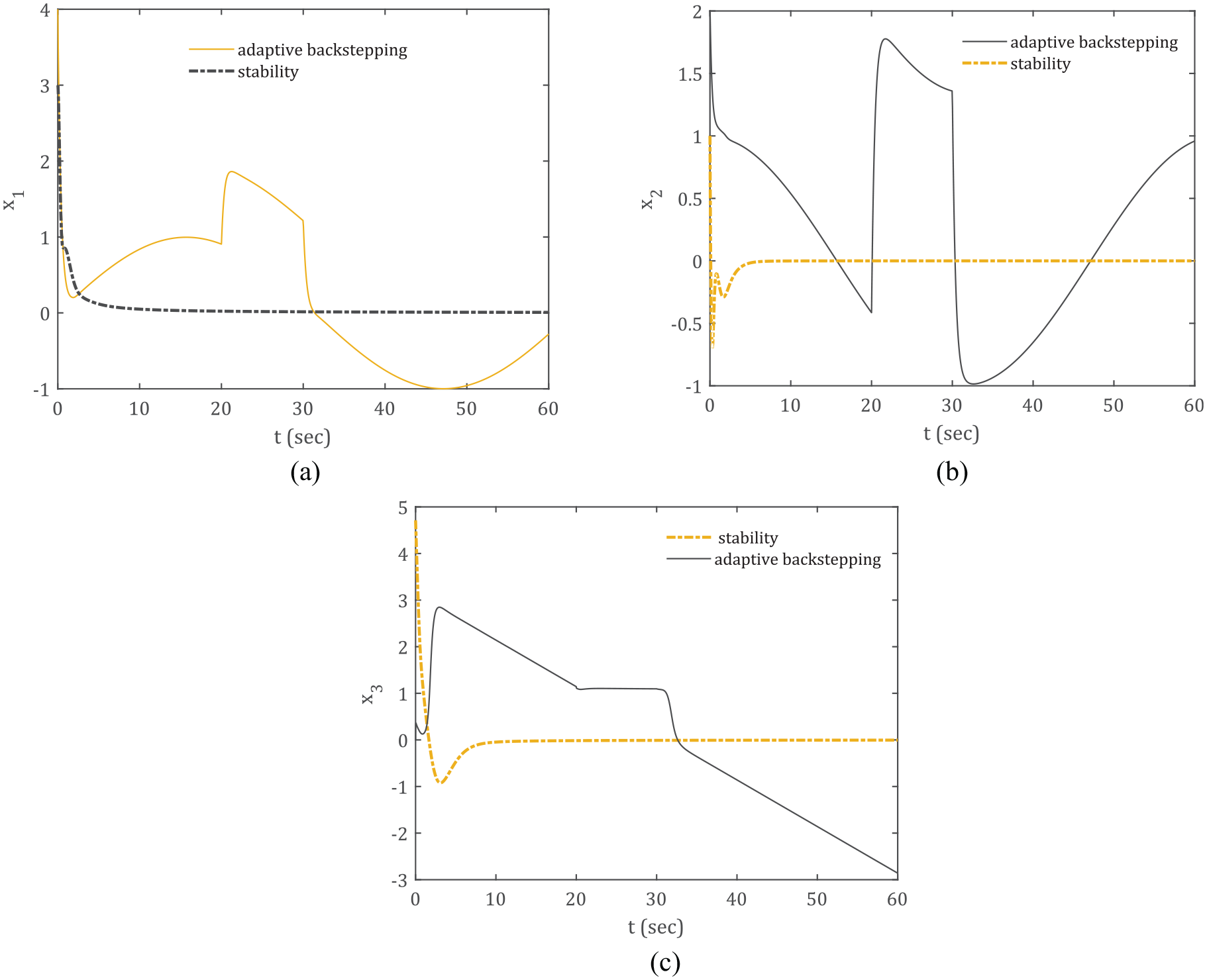
Time-history of steady space stabilization and adaptive backstepping in the presence of slip.

Finally, in Figure 16(a) and (b) according to equation (34) for reference paths considered in both backstepping control methods and stabilization of Lyapunov function, it can be seen that in each round of reference path in the range of applied adaptive rules Designed in the backstepping method with sudden changes and going through a longer path to compensate for the effects of slippage in the system, of course, it should be noted that in both methods the system has converged to the reference path, but in comparative rules the proposed method The reason for moment-to-moment correction of the difference between the system signals and the reference path signals has been very small changes in the slip interval, which is why the comparative law used in the proposed method is exactly an estimation method according to the kinematics of each system. It does not perform complex design and operations to obtain adaptive rules such as the backstepping method, which in the process of solving the problem we have to make assumptions and only model a part, because in the proposed method, the slip estimation method corresponds exactly to the kinematics and dynamics of the problem. And because of this the system easily slips even very large easily dismantles the system and brings the system to stability and convergence.

Figure 16.

Tracking of a path #1 and path #2 trajectory in presence of wheels’ slip stability estimator and adaptive estimator: (a) path #1 and (b) path #2.

Conclusion

In this paper, the stabilization problem of N-trailer wheeled mobile robot was examined. First, a kinematic discontinuous controller was designed based on the Lyapunov function model. This design of the controller is based on the dynamic system stabilization system of the system according to the principles and conditions considered in the system for the general design of a system based on Lyapunov function and in a special case for a wheeled mobile robot with three trailers. Simulation results are presented to show the performance of the designed controller.

The special method and stabilization in this article is such that it can be used for any desired axis to add the desired number of trailers by vehicle. Therefore, in this type of connection, it has more flexibility than the previous case and more trailers can be connected to the tractor for the desired purposes and purposes. However, in this method, because the trailer is pinned at a point outside the axis and the body of the tractor, it is more difficult to control, and in some cases, this type of connection causes system instability, which is more related to more than trailers are waiting for the tractor system. But the advantage of this type of connection over direct connection is that the connection between system inputs will be in the form of algebraic equations and very simple in the form of a matrix form that can solve problem time as well as simple calculations without the need to create a derivative. Create time between inputs and system dynamics for connection between previous and current inputs. ⁴⁵

The new idea used in this paper is to estimate the slip applied to the control inputs of the system with a new method that can estimate the slip well in most cases and solve complex adaptive, nonlinear, and equations. In Lyapunov functions, we estimate the slip system from the kinematic solution of the system and measure the signals of the state variables, and consider and measure all the uncertainties of the system in modeling. In fact, in this method we assume that the state variables x, y, θ measured a vehicle using a measured ${\mathrm{T}}_P$ distance using some receiver sensors (e.g. a visual system). ⁴⁶ With this assumption, the easiest way to obtain the values $({\delta }_1,{\delta }_2)$ to estimate them is from equation (2). In practice, the calculations calculated in this way are obtained from the following equations:

$$\begin{array}{c}{\hat{\delta }}_x\left(n\right)=\stackrel{·}{x}\left(\mathrm{n}\right)-u_3(n-1)\cos [{\theta }_3(n-1)+{\epsilon }_{\theta }(n-1)]+{\epsilon }_x(n-1)\hfill \\ {\hat{\delta }}_y\left(n\right)=\stackrel{·}{x}\left(\mathrm{n}\right)-u_3(n-1)\cos [{\theta }_3(n-1)+{\epsilon }_{\theta }(n-1)]+{\epsilon }_y(n-1)\hfill \end{array}$$

(35)

Where $\stackrel{·}{x}\left(n\right)=[x\left(n\right)-x(n-1)]/\mathrm{Tp},\stackrel{·}{y}\left(n\right)=[y\left(n\right)-y(n-1)]/\mathrm{Tp}$ and ${\epsilon }_y,{\epsilon }_x,{\epsilon }_{\theta }$ represents the random measurement noise that is always present in practical execution. If the measured noise increases the estimation variance, it can be filtered from the right (35) and the filtered components ${\hat{\delta }}_x^F,{\hat{\delta }}_y^F$ (filter estimator) can now be used instead. Actual signals $({\delta }_1,{\delta }_2)$ used skid estimates in the definitions that are not known in practice (more information on slip estimation in Keymasi Khalaji and Jalalnezhad ²⁹ ).

According to the results presented in the previous section, it can be seen that the back-stepping control method by connecting the N trailer off-axis and the algebraic equations resulting from the connections and also by adding the effect of wheel slip to the system kinematic equations as structural uncertainty and estimating this disturbance entered into the system and the lack of control and prediction of the control algorithm with this uncertainty, the real robot before stabilization the system malfunction and also following the desired path (reference) that without adaptive rules to estimate unknown system parameters in The sliding effect of the response to the path is disrupted and the process of tracking the reference path is disrupted. On the other hand, in the back-stepping control method, in the presence of the slip estimator due to the design of adaptive rules and estimation of each time of uncertainty, it is observed that at the time of disturbance according to the equations as slip, the robot at the moment applying this condition to follow the reference path can be deviated, but very quickly this disorder is compensated by adaptive rules and the robot compensates the reference path by eliminating the slip parameters and then in the direction of the reference path. Located, and conforms to the path. The results show that slip estimation in the presence of this type of structural uncertainty has a significant improvement in the tracking quality of reference paths. As we can see, for different reference paths, starting from different initial conditions, after a limited time, the wheeled mobile robot along with the trailer is placed in the reference path and in the shortest possible time, the slip effects with appropriate adaptive rules. Eliminates and when slipping is applied, error estimation will be applied to compensate and send a new signal to the system controller. The designed control inputs also have compatible conditions and stabilize the system to the point of reference, and show their efficiency within a reasonable range.