Sage Journals: Discover world-class research

Abstract

In the fault diagnosis of high-pressure common rail diesel engines, it is often necessary to face the problem of insufficient diagnostic training samples due to the high cost of obtaining fault samples or the difficulty of obtaining fault samples, resulting in the inability to diagnose the fault state. To solve the above problem, this paper proposes a small-sample fault diagnosis method for a high-pressure common rail system using a small-sample learning method based on data augmentation and a fault diagnosis method based on a GA_BP neural network. The data synthesis of the training set using Least Squares Generative Adversarial Networks (LSGANs) improves the quality and diversity of the synthesized data. The correct diagnosis rate can reach 100% for the small sample set, and the iteration speed increases by 109% compared with the original BP neural network by initializing the BP neural network with an improved genetic algorithm. The experimental results show that the present fault diagnosis method generates higher quality and more diverse synthetic data, as well as a higher correct rate and faster iteration speed for the fault diagnosis model when solving small sample fault diagnosis problems. Additionally, the overall fault diagnosis correct rate can reach 98.3%.

Keywords

Diagnostics diesel engine failure diagnosis genetic algorithm (GA)neural network

Introduction

With the large-scale use of high-pressure common rail diesel engines, their maintenance and fault diagnosis problems have become increasingly severe. As a complex system consisting of a high-pressure oil pump, common rail pipe, electronically controlled injector, and high-pressure fuel pipe, a high-pressure common rail system is susceptible to various failures during operation due to shock and vibration, wear, corrosion, and aging. In recent years, wavelet analysis, empirical mode decomposition (EMD), ensemble empirical mode decomposition (EEMD),^1–8 and other time domain analysis methods have been widely used in the analysis and diagnosis of diesel engine faults.^9–12 In the field of eigenvalue identification, energy entropy, permutation entropy, singular values, and time-domain features are applied to the extraction of feature parameters.^13–19 In a classification and combination problem, classification algorithms such as support vector machines and neural networks are used in fault diagnosis. However, the use of the above fault diagnosis methods presupposes the availability of large amounts of different operating data for training in classification. Not enough data are available for all operating conditions, especially for complex power machinery such as high-pressure common rail diesel engines, for which the data for certain operating conditions do not have the basis and conditions for large-scale acquisition. There are four main reasons that prevent the large-scale acquisition of data, as follows.

Some failures only occur in specific environments or working conditions, and it is difficult for the bench test to simulate the occurrence environment and working conditions of such failures.

The cause and mechanism of some failures are not clear, and the bench test cannot simulate the occurrence of such failures.

The cost of a bench test for simulating some failures is too high to obtain large-scale operation data.

Some failures are destructive, and the simulation of this failure may cause damage to the bench test and even the test personnel.

When a large amount of operating data for a fault cannot be obtained for some reason, determining how to use a small amount of operating data for fault diagnosis becomes an urgent problem, namely, the small sample fault diagnosis problem referred to in this paper. Traditional methods mainly obtain large amounts of data through the establishment of simulation models, but there are always errors between the simulation data and the real data, and the diversity of the simulation data is weak and unable to fully demonstrate the characteristic parameters of the state. After in-depth study of the fault diagnosis of a high-pressure common rail system, this article divides this problem into two aspects: the first aspect is the solution to the problem of small sample learning, that is, determining how to use a small amount of data to complete the training of the fault diagnosis model; the second aspect is determining how to improve the diagnosis accuracy and speed of the fault diagnosis model that uses a small amount of data for fault diagnosis.

For the first aspect, the problem of single-sample learning was noticed by some researchers in the 1980s. In 2003, Li et al. introduced the concept of small-sample learning.^20–23 Depending on the different methods used, there are three main types of small-sample learning: model-based fine-tuning, data-based enhancement, and migration-based learning. Model fine-tuning-based approaches first train a classification model based on a source dataset containing a large amount of data and then fine-tune the model on a target dataset containing a small amount of data. However, this approach may lead to the overfitting of the model because a small amount of data does not accurately reflect the true distribution of a large amount of data. The method based on transfer learning is currently a more cutting-edge approach, but it still has problems such as low accuracy when the sample is too small, or high complexity, immature algorithms, or high computational complexity when the sample dimension becomes large. While small sample learning methods based on data enhancement may introduce noise and other negative effects, these problems can be solved by improving the performance of the diagnostic model. Additionally, given that sufficient training data is available for most faults, data enhancement-based small-sample learning, especially data synthesis-based small-sample learning, can be used to obtain a large amount of synthetic data and share a fault diagnosis model with other faults, which helps to reduce the complexity of a system.^24–26

The data synthesis based approach refers to the collection of small sample data into new labeled data to expand the training data.²⁷ Mehrotra et al. proposed the application of a generative adversarial network (GAN) to small sample learning by training two mutually adversarial neural networks to synthesize data, but the quality of the synthesized data was not very satisfactory. To improve the performance of GANs, scholars have made various improvements to the architecture of GANs in recent years. Radford et al. proposed a deep convolutional generative adversarial network (DCGAN) by applying a convolutional neural network to GAN architecture. Mirza and Osindero proposed a conditional generative adversarial network (CGAN) that used conditional variables as additional information to constrain the generative process. Chen et al. proposed an interpretable representation learning by information maximizing generative adversarial network (Info GAN) that split structured hidden variables from a noise vector as conditional variables to control the outcome of the generated images. Furthermore, there are excellent GAN architectures such as Bi-GAN, ALI, VAE, etc. which are widely used in various fields.^28–31 However, some of the above architectures are less stable in the training process, especially when small batch sample training is not available at all. Small-sample learning in fault diagnosis is intended to provide a diagnostic model with sufficient and high-quality training data that can adequately describe the operational state. Therefore, in addition to the generation quality of the GAN, the synthesized data should be highly diverse. Among various architectures, least squares generative adversarial networks (LSGANs) proposed by Goodfellow have obtained synthetic data with high quality and diversity by replacing the cross-entropy loss function with the least squares loss function.³² In this research, based on the LSGAN architecture, we use EMD to evaluate the similarity between the synthetic data and the real data, and in order to prevent the synthetic data from being too similar to the real data and reducing the diversity of the data, we set an iteration stopping condition so that the network stops iterating at an appropriate time to synthesize the training sample set.

For the second aspect, there are already models such as SVM, random tree forest, and neural network classifier models that can be used as fault diagnosis models. Among these models, the back propagation (BP) neural network^33–37 is a multilayer feedforward network using an error back propagation algorithm for learning. This neural network can implement complex nonlinear mapping functions and compute results with high accuracy. Compared with other prediction methods, the BP neural network model is one of the most frequently used and mature neural network models because of its simplicity and high fault tolerance to data. Although the BP neural network has a wide range of applications, it still has problems such as low learning efficiency and slow convergence, and the initial weights and thresholds are randomly generated by the network during the training process, which can easily cause the network to fall into a local optimum. To improve the convergence speed, avoid falling into local optimum solutions, and improve the performance of fault diagnosis models, in this research, an improved genetic algorithm is used to initialize the BP neural network. The genetic algorithm can effectively solve the optimization problem by simulating the genetic process in biological evolution. It screens the individuals of the population through selection, crossover, and mutation, leaving the individuals with high fitness and eliminating those with poor fitness, and it continuously iterates the evolution until the individuals satisfying the conditions are obtained.

Based on the above methods, in this research the small sample learning method based on data synthesis to synthesize training data for fault diagnosis model training, and the BP neural network initialized by the genetic algorithm is used for fault diagnosis. In order to optimize the performance of the genetic algorithm, Adaptive random testing (ART) is used to initialize the relevant parameters of the genetic algorithm, and the genetic and mutation rate is changed by an adaptive method to achieve the purpose of optimizing the genetic algorithm, making the initial value passed by the genetic algorithm to the BP neural network better and effectively increasing the convergence speed of the BP neural network, improving the accuracy of the fault diagnosis model. The fault diagnosis process is shown in Figure 1.

Figure 1.

Flowchart of small sample fault diagnosis of high-pressure common rail system.

Extraction and pre-processing of rail pressure signal

The fault diagnosis of a high-pressure common rail system is generally based on vibration and vibro-acoustic signals, assisting other operating parameters in the extraction and construction of the eigenvalue and eigenvector. Because the vibration and vibro-acoustic generated in the operation of a high-pressure common rail fuel supply system are small, it is extremely difficult to accurately extract and construct the eigenvector of a high-pressure common rail fuel supply system with traditional methods. In a common rail fuel supply system, a common rail pipe is an important component connecting the high-pressure fuel pump, injector, and other parts, and the common rail pipe pressure contains a large amount of information, so the eigenvector of a common rail fuel supply system can be extracted and constructed using the rail pressure. In this research, a 10-cylinder diesel engine high-pressure common rail system is taken as the research object. To simplify the calculation, a five-cylinder monorail diesel engine high-pressure common rail fuel supply system bench is built for research. The test system consists of a Delphi high-pressure common rail fuel injection system, Hansmann 22 kW fuel injection pump test bench, EMI-II transient parameter test and analysis system, EFS8233 common rail injector solenoid valve controller, EFS8244 orbital pressure controller, orbital pressure sensor, high precision angle sensor, and high strength coupling. A schematic sketch and an experimental diagram are shown in Figures 2 and 3. Figure 3(a) is the physical map of the experimental bench composed of a fuel pump, common rail pipe, and fuel injector, and Figure 3(b) is the physical map of the control device and the host computer.

Figure 2.

Schematic diagram of the common rail test set system.

Figure 3.

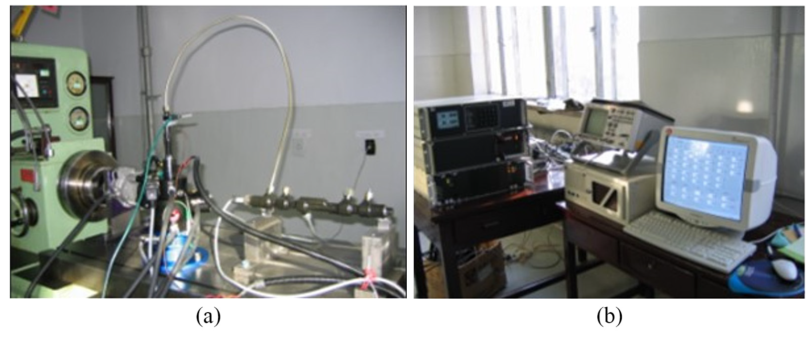
Test scene of common rail system: (a) experimental bench and (b) the control device and the host computer.

After extracting the rail pressure signal, the rail pressure sensor is susceptible to the influence of the including system, environment, and other high frequency noise. To improve the quality of the rail pressure signal, in this research, a first-order low-pass analog filter is used for the pre-processing of the rail pressure signal with a time constant of 450 μs and a transfer function, as shown in equation (1). This filter can effectively eliminate high-frequency noise at frequencies above 350 Hz.³⁸

H (s) = \frac{1}{1 + T \cdot s}

(1)

To solve the problems of signal damage and loss during rail pressure signal acquisition, unify the rail pressure signal step length, and improve the quality of the rail pressure signal, in this research linear interpolation is used to process the collected rail pressure signal. This is an interpolation method based on an iterated function system (IFS). The interpolation method can reflect the characteristics of the local fluctuations between the interpolation points, and it has higher accuracy than the traditional interpolation methods in describing the curves of nonlinear changes.³⁹

It is assumed that there is a set of interpolated data, as shown in equation (2):

\begin{matrix} D = {(x_{i}, y_{i}) \\ \in I \times R, i = 1, 2, 3 \dots N} \\ x_{1} < x_{2} < x_{3} < \dots < x_{N} \\ I = [x_{1}, x_{N}] \end{matrix}

(2)

The interpolation function f(x) has $f (x_{i}) = y_{i}$ for every $x_{i}$ , and the interpolated data ( $x_{i}$ , $y_{i}$ ) are not collinear.

The attractor G = {(x,f(x)), $x \in (x_{0}, x_{N})}$ is the continuous image of the interpolated data.

It is assumed that $W_{i}$ is the mapping function, as shown in equation (3):

\begin{matrix} W_{i} (\begin{matrix} x \\ y \end{matrix}) = (\begin{matrix} a_{i} & b_{i} \\ c_{i} & d_{i} \end{matrix}) (\begin{matrix} x \\ y \end{matrix}) + (\begin{matrix} e_{i} \\ f_{i} \end{matrix}) \\ i = 1, 2, 3 \dots N \end{matrix}

(3)

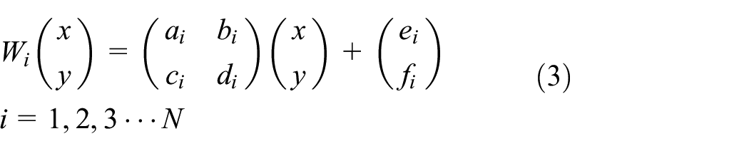
and the conditions are met, as shown in equation (4):

{\begin{matrix} W_{i} (\begin{matrix} x_{0} \\ y_{0} \end{matrix}) = (\begin{matrix} x_{i - 1} \\ y_{i - 1} \end{matrix}) \\ W_{i} (\begin{matrix} x_{N} \\ y_{N} \end{matrix}) = (\begin{matrix} x_{i} \\ y_{i} \end{matrix}) \end{matrix}

(4)

According to the conditions of the IFS, the mapping function can be derived:

{\begin{matrix} \begin{matrix} a_{i} = \frac{x_{i} - x_{i - 1}}{x_{N} - x_{0}} \\ b_{i} = 0 \\ c_{i} = \frac{y_{i} - y_{i - 1}}{x_{N} - x_{0}} - d_{i} \frac{y_{N} - y_{0}}{x_{N} - x_{0}} \end{matrix} \\ \begin{matrix} | d_{i} | < 1 \\ e_{i} = \frac{x_{N} x_{i - 1} - x_{0} x_{i}}{x_{N} - x_{0}} \end{matrix} \\ f_{i} = \frac{x_{N} y_{i - 1} - x_{0} y_{i}}{x_{N} - x_{0}} - d_{i} \frac{x_{N} y_{0} - y_{N} x_{0}}{x_{N} - x_{0}} \end{matrix}

(5)

In equation (5), $d_{i}$ is a free variable called the vertical scale factor, and the interpolation function in the vicinity of the attractor G is iterated to complete the fractal interpolation fitting. After extraction, the pre-processed rail pressure signal is as shown in Figure 4.

Figure 4.

Rail pressure signal.

LSGAN-based rail pressure data synthesis

As powerful generative networks, GANs are widely used in fields such as image generation, data enhancement, and sample generation. A GAN is composed of two deep neural networks, a generative model (G) and discriminative model (D). The loss function of a traditional GAN can be expressed as:

\begin{matrix} \begin{matrix} \min \\ G \end{matrix} \begin{matrix} \max \\ D \end{matrix} V (D, G) = E_{x ~ p_{data}} [logD (x)] + E_{z ~ p_{z}} \\ [\log (1 - D (G (z)))] \end{matrix}

(6)

where $p_{data}$ is the probability distribution of the real data, $p_{z}$ is the probability distribution of the data generated according to the noise, E is the expectation, and z is the noise. The generative model and the discriminative model in the generative adversarial network oppose each other, the goal of the generative model is to generate synthetic data as similar as possible to the real data, and the discriminative model is used to determine whether the target is the real data. The traditional GAN structure is shown in Figure 5. The GAN trains the generative model G and the discriminant model D with a loss function and learns the distribution of the real data.

Figure 5.

Traditional GAN structure.

A diagram of the probability-based training process of GAN is shown in Figure 6. In the figure, the dotted, dashed, and solid lines indicate the distribution of the real data, the distribution of the synthetic data, and the discriminative model, respectively, and the arrows indicate how the generator G converts the input noise into synthetic data.

Figure 6.

Training schematic: (a) initial distribution, (b) training D, (c) training G, and (d) reaching balance.

In solving the small sample fault diagnosis problem of high-pressure common rail faced in this research, in order to improve the quality and diversity of the synthetic data, least squares is used as the loss function instead of cross entropy and a generative adversarial network with higher diversity is constructed using different distances instead of distribution probabilities as the measure. The loss function is shown in equation (7).

\begin{array}{l} {{}_{D}^{m i n}V}_{L S G A N} (D) = \frac{1}{2} E_{x ~ p_{data}} (x) [{(D (x) - b)}^{2}] \\ + \frac{1}{2} E_{x ~ p z (z)} (z) [{(D (G (z)) - a)}^{2}] \\ {{}_{G}^{m i n}V}_{L S G A N} (G) = \frac{1}{2} E_{x ~ p z (z)} (x) [{(D (G (z)) - c)}^{2}] \end{array}

(7)

where $p_{data}$ is the probability distribution of the real data, $p_{z}$ is the probability distribution of the data generated from the noise, E is the expectation, z is the noise, and a, b, and c are constants. In this research, we use the binary labels 0–1, where the constants b = c = 1 and a = 0.

To prevent the synthetic data from being too similar to the real data and to reduce the diversity of the data, the iteration stopping condition is set as shown in equation (8).

\begin{matrix} \frac{1}{k (k - 1)} \sum_{q = 1}^{k} \sum_{w = 1, q \neq w}^{k} EMD (q, w) \geq \max Π_{d = 1}^{p} \\ \min Π_{s = 1}^{k} EMD (d, s) \land V \leq v \end{matrix}

(8)

where k is the number of the input real data, p is the number of the output synthetic data, and $EMD (q, w)$ is the $EMD$ of the qth input data and the wth input data, which is an algorithm used to calculate the distance between two geometric or vectorial data with the linear programing of one order. The $EMD$ has a wide application in assessing the discrepancy of two multidimensional distributions.⁴⁰ For any two spatial curves, the smaller the $EMD$ value is, the higher the similarity is and the smaller the difference is, and vice versa; the lower the similarity is, the higher the difference is. $EMD (s, d)$ is the $EMD$ of the sth input data and the dth output data, V is the minimum number of iterations, and v is the current number of iterations. When the above inequality is satisfied, it means that the average $EMD$ for the synthetic data and the real data is less than or equal to the average $EMD$ for the real data, at which time stopping the iteration can produce synthetic data with good diversity.

It is assumed that there are two sets of eigenvectors, as shown in the following equation:

\begin{matrix} X = {(x_{1}, W_{x_{1}}), (x_{2}, W_{x_{2}}), (x_{3}, W_{x_{3}}), \dots (x_{m}, W_{x_{m}})} \\ Y = {(y_{1}, W_{y_{1}}), (y_{2}, W_{y_{2}}), (y_{3}, W_{y_{3}}), \dots (y_{n}, W_{y_{n}})} \\ \sum_{i = 1}^{m} W_{x_{i}} = \sum_{j = 1}^{n} W_{y_{j}} \\ x_{i} \in R^{H}, y_{j} \in R^{H}, W_{x_{i}} \in R, W_{y_{j}} \in R \end{matrix}

(9)

where $x_{i} and y_{j}$ represent the eigenvalues of the two rail pressure signals, and $W_{x_{i}} and W_{y_{j}}$ represent the weights of the corresponding eigenvalues. $f_{ij}$ is obtained by solving the optimal solution in equation (10):

\begin{matrix} \min \sum_{i = 1}^{m} \sum_{j = 1}^{n} d_{ij} f_{ij} \\ s . t \\ f_{ij} \geq 0 (i = 1, 2, \dots m; j = 1, 2, \dots n) \\ \sum_{i = 1}^{m} f_{ij} \leq W_{y_{j}} (j = 1, 2, \dots n) \\ \sum_{j = 1}^{n} f_{ij} \leq W_{x_{i}} (i = 1, 2, \dots m) \\ \sum_{i = 1}^{m} \sum_{j = 1}^{n} f_{ij} = \min {\sum_{i = 1}^{m} W_{x_{i}}, \sum_{j = 1}^{n} W_{y_{j}}} \end{matrix}

(10)

In equation (10) $d_{ij}$ is the distance between $x_{i}$ and $y_{i}$ . According to the above expression, the EMD of the two rail pressure signals is obtained as:

EMD (X, Y) = \frac{\sum_{i = 1}^{m} \sum_{j = 1}^{n} d_{ij} f_{ij}}{\sum_{i = 1}^{m} \sum_{j = 1}^{n} f_{ij}}

(11)

For the characteristics of the rail pressure signal, equation (10) is modified as follows:

\begin{matrix} x_{i} = (P_{x_{i}}, T_{i x_{i}}) (i = 1, 2, \dots m) \\ y_{j} = (P_{y_{j}}, T_{y_{j}}) (j = 1, 2, \dots n) \\ W_{x_{i}} = W_{y_{j}} (i = 1, 2, \dots m; j = 1, 2, \dots n) \end{matrix}

(12)

In equation (12), $P_{x_{i}}$ represents the ith rail pressure minima of the rail pressure signal X, and $T_{i x_{i}}$ is its corresponding time. $P_{y_{j}}$ represents the jth rail pressure minima of the rail pressure signal Y, and $T_{y_{j}}$ is its corresponding time. The $d_{ij}$ in equation (10) is shown in the following equation:

d_{ij} = \sqrt[2]{P_{x_{i}} - {P_{y_{j}}}^{2} + T_{i x_{i}} - {T_{y_{j}}}^{2}}

(13)

To improve the convergence speed and prevent the generator from simply copying the original sample, the rail pressure signal is randomly intercepted without fuel injection, as shown in Figure 7, with a fixed length as the input signal. This is input to the generator G. Through several experimental observations and analyses, it is found that the best quality and diversity of the synthesized rail pressure signal is achieved when the Adam optimizer is used in generator G.

Figure 7.

Rail pressure signal when no fuel is injected.

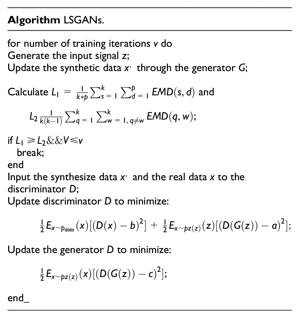
In summary, an improved LSGAN is built, for which the generator G is a BP neural network with one hidden layer. The LSGAN has 60 input layer nodes, 100 hidden layer nodes, and 473 output layer nodes. The rule output layer uses the tanh function as the activation function, and all the other layers use ReLU as the activation function. The neural network has BN layer and uses the Adam optimizer to adjust the hyperparameters. The discriminator D is a BP neural network with one hidden layer. It has 473 input layer nodes, 100 hidden layer nodes, and 1 output layer node. All of the layers use LeakyReLU as the activation function. The slope is 2, the learning efficiency is 0.05, and the minimum number of iterations is 50,000. Every 100 generations, it is determined whether to meet the stop iteration condition. To facilitate the calculation, all of the EMD calculations described in this paper use the normalized signal. The algorithm pseudo-code is as follows:

Algorithm LSGANs.
for number of training iterations v do Generate the input signal z; Update the synthetic data $x^{,}$ through the generator G; Calculate $L_{1} = \frac{1}{k * p} \sum_{s = 1}^{k} \sum_{d = 1}^{p} EMD (s, d)$ and $L_{2} \frac{1}{k (k - 1)} \sum_{q = 1}^{k} \sum_{w = 1, q \neq w}^{k} EMD (q, w)$ ; if $L_{1} \geq L_{2} & & V \leq v$ break; end Input the synthesize data $x^{,}$ and the real data x to the discriminator D; Update discriminator D to minimize: $\frac{1}{2} E_{x ~ p_{d a t a}} (x) [{(D (x) - b)}^{2}] + \frac{1}{2} E_{x ~ p z (z)} (z) [{(D (G (z)) - a)}^{2}];$ Update the generator D to minimize: $\frac{1}{2} E_{x ~ p z (z)} (x) [{(D (G (z)) - c)}^{2}]$ ; end_

Algorithm LSGANs.

for number of training iterations v do
Generate the input signal z;
Update the synthetic data

x^{,}

through the generator G;
Calculate

L_{1} = \frac{1}{k * p} \sum_{s = 1}^{k} \sum_{d = 1}^{p} EMD (s, d)

and

L_{2} \frac{1}{k (k - 1)} \sum_{q = 1}^{k} \sum_{w = 1, q \neq w}^{k} EMD (q, w)

;
if

L_{1} \geq L_{2} & & V \leq v

break;
end
Input the synthesize data

x^{,}

and the real data x to the discriminator D;
Update discriminator D to minimize:

\frac{1}{2} E_{x ~ p_{d a t a}} (x) [{(D (x) - b)}^{2}] + \frac{1}{2} E_{x ~ p z (z)} (z) [{(D (G (z)) - a)}^{2}];

Update the generator D to minimize:

\frac{1}{2} E_{x ~ p z (z)} (x) [{(D (G (z)) - c)}^{2}]

;
end_

Common rail system fault diagnosis model

To verify the accuracy of the synthetic data, in this research, EEMD is used to decompose the rail pressure signal into different intrinsic modal functions (IMFs) to construct the eigenvectors using energy entropy and to establish an improved GA_BP neural network as a common rail system fault diagnosis model for fault diagnosis.

EEMD-based rail pressure signal decomposition and eigenvalue extraction

EEMD is a proposed method based on EMD that is used to decompose the signal into intrinsic modal functions. By adding a white noise signal to the original signal, the signals of different time scales are distributed to a suitable reference scale, and the final result is obtained by integrating the mean value after several instances of average noise canceling. EEMD solves the modal mixing problem that exists in EMD using the characteristic of the uniform distribution of the white noise signal spectrum, further improves the accuracy of decomposition, and more accurately retains the features in the original data. The decomposition flow chart of EEMD is shown in Figure 8.^17,18

Figure 8.

EEMD flow chart.

In the process of fitting the curve to obtain the upper and lower envelopes, in this research, the third spline interpolation curve is used to construct the envelope. It is assumed that the interval [a,b] has: $a = x_{0} < x_{1} < \dots < x_{n} = b$ , and for i = 1,2,3,⋯, n − 1 we have the following equation.

{\begin{matrix} s_{i} (x_{i} - 0) = s_{i} (x_{i} + 0) = f (x_{i}) \\ s_{i} (x_{i + 1} - 0) = s_{i} (x_{i + 1} + 0) = f (x_{i + 1}) \\ s_{i}^{,} (x_{i} - 0) = s_{i} (x_{i} + 0) = 0 \\ s_{i}^{,} (x_{i + 1} - 0) = s_{i} (x_{i + 1} + 0) = 0 \end{matrix}

(14)

The iterative stop function is shown in equation (15):

a (t) = \frac{| e_{\max} + e_{\min} |}{| e_{\max} - e_{\min} |}

(15)

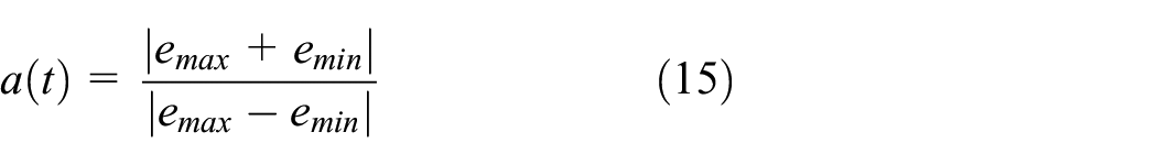
In equation (15), $e_{\max} and e_{\min}$ are the upper and lower envelopes, respectively. Three threshold values $θ_{1}, θ_{2}, and α$ are set. The iteration is ceased when the proportion of a(t) less than $θ_{1}$ is not less than α and there is no value greater than $θ_{2}$ . After applying EEND to the rail pressure signal decomposition, to construct the feature vector, the IMF components are selected with the over-zero rate curve to extract the feature parameters.

The energy of each IMF component represents the energy of the signal in this frequency, so there is some kind of mapping relationship between the signal and the energy, which can be used as a basis for fault diagnosis. The corresponding energy is extracted for IMF1–IMF3 to construct the eigenvectors.^19–21 The energy $E_{i}$ of each IMF component is:

E_{i} = \int_{0}^{T} c_{i}^{2} dt i = 1, 2, 3

(16)

In equation (16), $E_{i}$ denotes the energy of the ith IMF and $c_{i}$ denotes the value of the ith IMF curve.

Improved GA_BP neural network fault diagnosis model

As a multilayer feedforward network with backpropagation error for learning, a BP neural network can achieve complex nonlinear mapping functions, which adjust weights and thresholds in the negative gradient direction of the cost function with the gradient descent valve method^22–26 to sequentially find the minimum value of a cost function and complete the training of a neural network. To accelerate the learning efficiency and convergence speed of the BP neural network and avoid falling into local optimal solutions, an improved genetic algorithm is used in this research to optimize the initial weights and thresholds of the BP neural network. The process of initializing the BP neural network using the genetic algorithm is shown in Figure 9.

Figure 9.

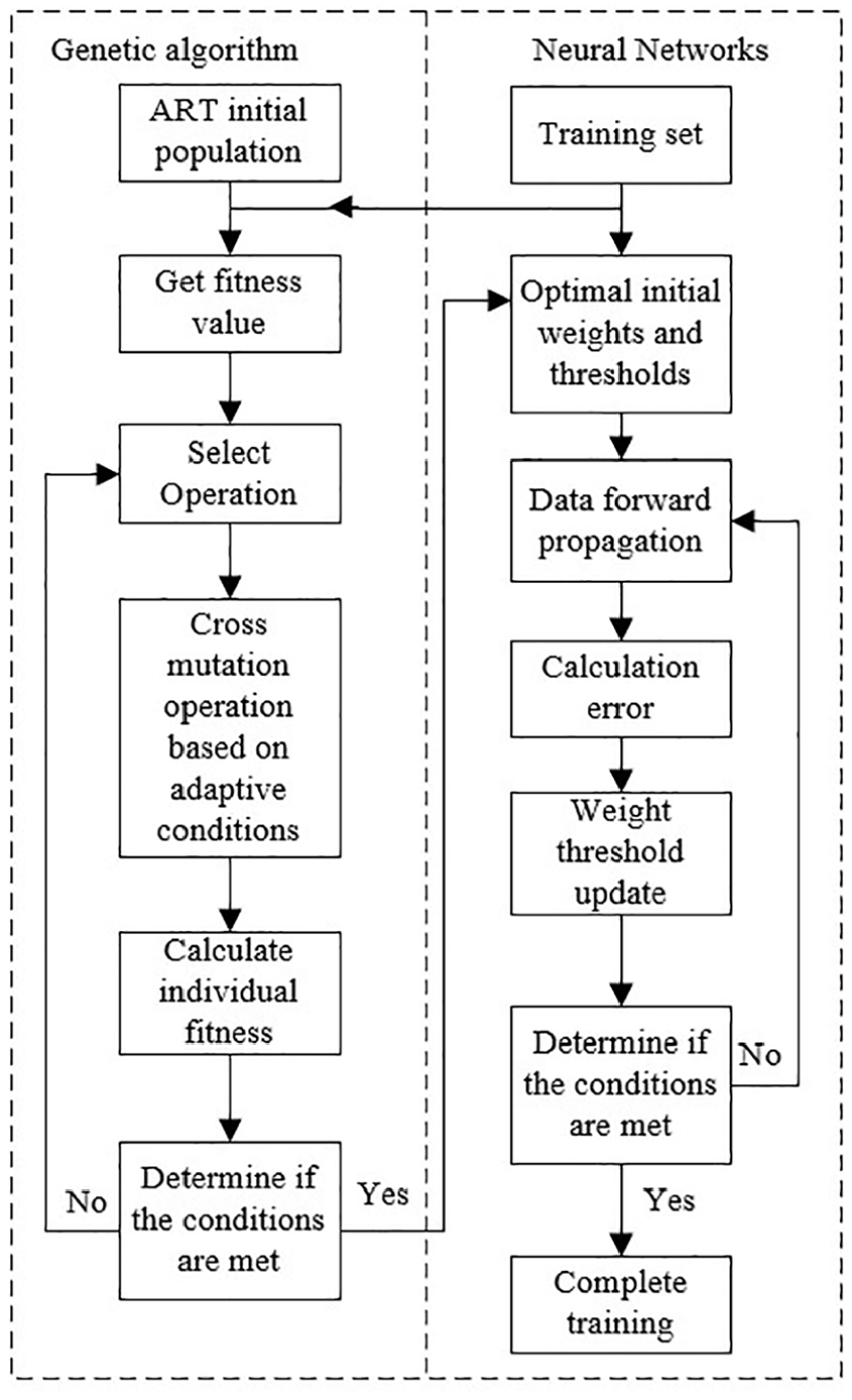
Flow chart of initialized neural network.

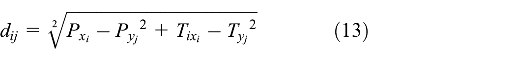
To increase the population diversity and avoid the optimization process from falling into local optimal solutions, the population initialization of the genetic algorithm is performed using the FSCS-ART algorithm. ART is an adaptive random testing algorithm. D-ART is one of the best ART testing algorithms, and its core concept is to first generate a candidate test set by calculating the shortest distance between each individual in the candidate test set and each individual in the test set, and then update the largest of the shortest distance to the test set.⁴¹ The fixed sized candidate set adaptive random testing (FSCS-ART) algorithm is one of the most classical algorithms in a series of D-ARTs, and its mathematical expression is shown in equation (17) as:

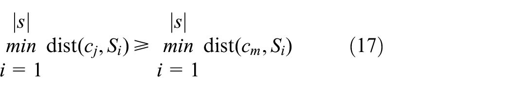
\begin{matrix} | s | \\ \min \\ i = 1 \end{matrix} dist (c_{j}, S_{i}) \geq \begin{matrix} | s | \\ \min \\ i = 1 \end{matrix} dist (c_{m}, S_{i})

(17)

In the formula, dist(a,b) represents the distance between two bodies a and b.

In the formula, n is the number of parameters to be initialized in the BP neural network. Figure 10 is a comparison diagram of a two-dimensional array of positive integers within 100 obtained using ART and a random number generator. From the figure, it can be seen that the data generated using ART is more uniform in distribution.

Figure 10.

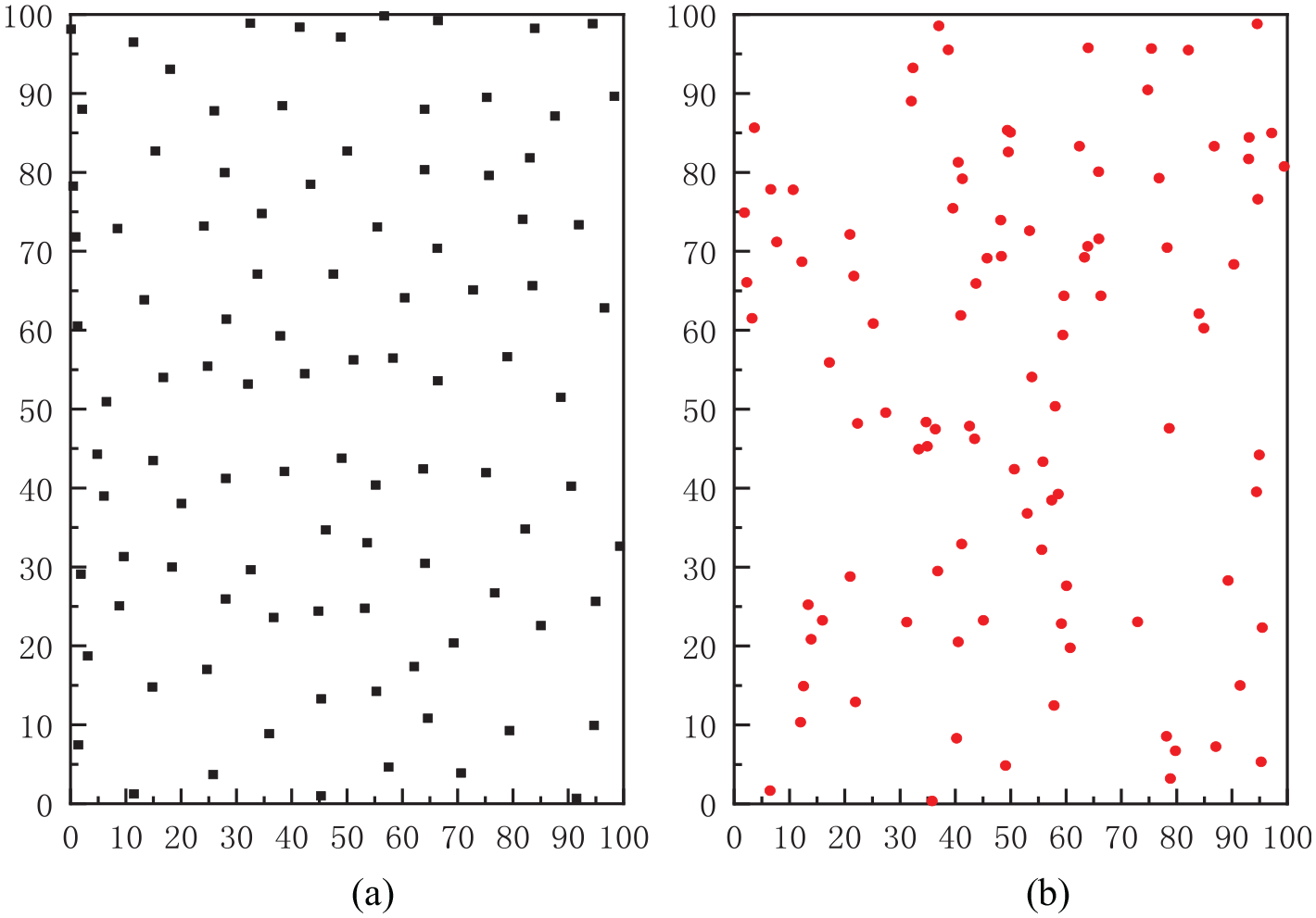
Comparison of: (a) ART and (b) randomly generated.

In the genetic algorithm, the offspring individuals are inherited from the parent individuals with fixed crossover and variation. For the BP neural network initialization problem in common rail system fault diagnosis, to speed up the convergence of the genetic algorithm, the evolutionary process of the population is divided into the early stage and the late stage. In the early stage of evolution, the population is genetically evolved with fixed crossover and variation rates to ensure the diversity of the population and to avoid optimization into local optimal solutions. In the late stage of evolution, the crossover and variation rates are altered via distance-based adaptive methods.^29–34

In this research, the total error function, as shown in equation (18) is used as an evaluation index of the individual fitness.

E = \frac{1}{2} \sum_{n = 1}^{N} \sum_{k = 1}^{z} {(T_{k}^{n} - Q_{k}^{n})}^{2}

(18)

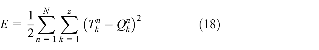
where N is the total number of input samples of the neural network, $Q_{k}$ is the actual output value of the kth node of the output layer, $T_{k}$ is the label of the input sample at the kth node, and z is the number of nodes of the output layer.

Based on the calculation of individual fitness, the probability of adaptive crossover and variation can be calculated as follows:

p_{c} = {\begin{matrix} k_{1}, f_{c} \leq f_{avg} \\ \frac{k_{1} (f_{\max} - f_{avg})}{f_{\max} - f_{avg}}, f_{c} \leq f_{avg} \end{matrix}

(19)

p_{m} = {\begin{matrix} k_{2}, f_{m} \leq f_{avg} \\ \frac{k_{3} (f_{\max} - f_{avg})}{f_{\max} - f_{avg}}, f_{m} \leq f_{avg} \end{matrix}

(20)

where $p_{c} and p_{m}$ are the probabilities of crossover and variation, respectively, $k_{1}, k_{2}, and k_{3}$ are the crossover and variation constants, $f_{c}$ is the fitness value of the individual with the greater fitness in the two bodies that perform the crossover, $f_{m}$ is the fitness value of the individual to be mutated, $f_{\max}$ is the maximum fitness of the population individuals, and $f_{avg}$ is the average fitness of the population individuals, which is calculated as shown in equation (21):

f_{avg} = \frac{\sum_{i = 1}^{N} E}{N},

(21)

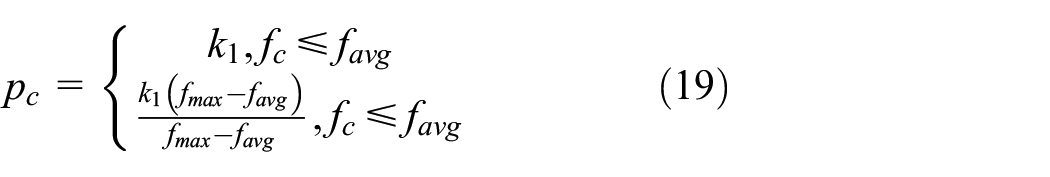
where N is the number of individuals in the population and E is the total error function.

Combining the above, a neural network with a learning efficiency of 0.1, a maximum number of 100 iterations and a structure of 3–8–4 is established, and the sigmoid function is chosen as the activation function of the hidden layer and the output layer. The initialization of the BP neural network by the improved genetic algorithm sets the population size to 20, the evolutionary generation to 40, the initial crossover probability to 0.9, and the initial variation probability to 0.1. According to the computational experience of the improved genetic algorithm, the best convergence effect and a more uniform distribution of the optimized solutions are achieved when the number of generations of the pre-late partition is set to 18.

Experiments and results analysis

According to the common faults of a common rail diesel engine fuel supply system and its classification, in this research, four operating states are selected for analysis, one of which is the normal operating state and three of which are fault states. The four operating states are the normal state, the second injector delayed injection state, the second injector solenoid valve wear state, and the high-pressure pump plunger wear state. The above four operating states are named state 1, state 2, state 3, and state 4. Fifty sets of rail pressure signals are collected for each of the above four operating states, and each set of rail pressure signals is an injection cycle. Since a large amount of data is required to verify the correct diagnosis rate and compare the quality of data generation, in this research, state 2, that is, the second injector delayed injection state, is selected as the fault state when it is difficult to obtain a large number of fault samples. The rail pressure signals of the four states are shown in Figure 11.

Figure 11.

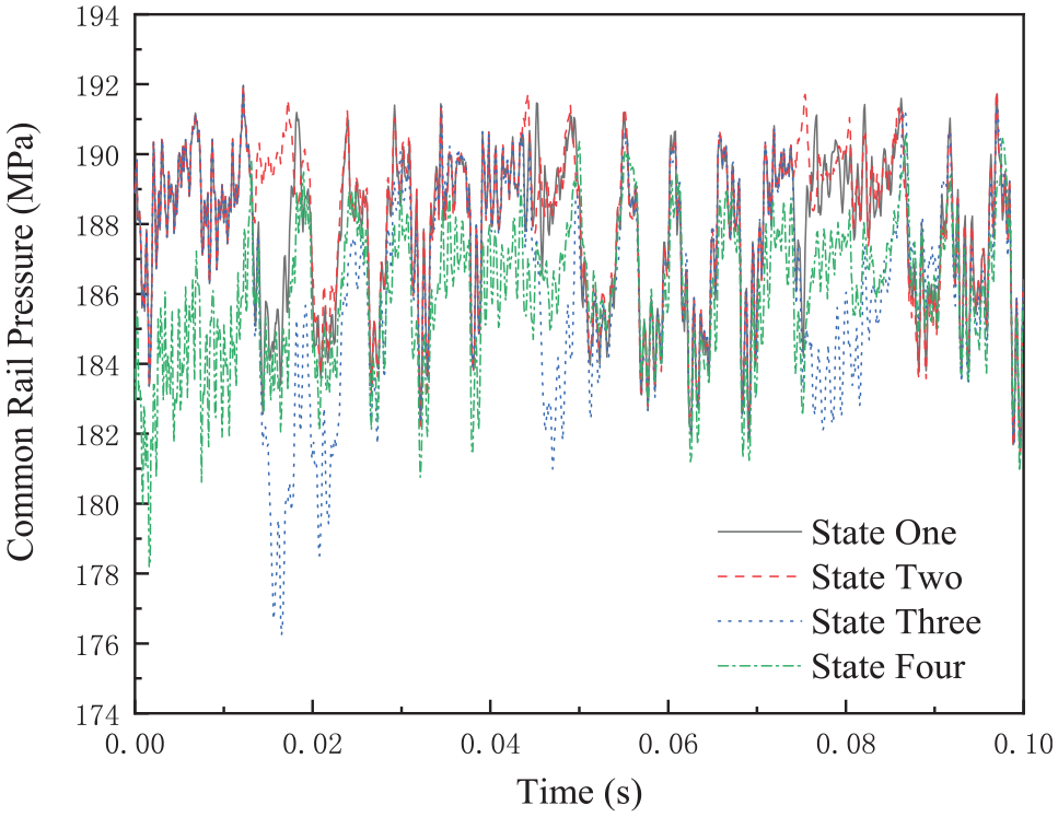
Rail pressure signals for different operating conditions.

When setting up the fault classification table, generally, when using the Sigmoid function the labels are set to the upper and lower bounds of their values, that is, 0.00 and 1.00, but in the actual training it is found that since the upper and lower bounds are not the target values of the activation function, there is a risk of generating too much weight when training the network. Therefore, 0.01 and 0.99 are chosen as the classification labels, based on which the fault classification table is as shown in Table 1:

Table 1.

Fault classification table.

Operationstatus	Faulttype	Tags
1	Normal	[0.99,0.01,0.01,0.01]
2	No. 2 injector delayedfuel injection	[0.01,0.99,0.01,0.01]
3	No. 2 injector solenoidvalve worn	[0.01,0.01,0.99,0.01]
4	High pressure fuel pumpplunger wear	[0.01,0.01,0.01,0.99]

In this research, MATLAB R2016b is used to build a rail pressure signal synthesis model and fault diagnosis model. The running environment is Win10, and the workstation configuration is as follows: Intel C621 series chipset, Intel Xeon Gold 6145 processor with 40 cores and 80 threads, main frequency of 2.0 GHz, maximum core frequency of 3.7 GHz, 128 GB RAM, and NVIDIA GT1030 2 GB graphics card.

Three sets of rail pressure signals for state 2 are randomly selected as real signals and input into the LSGANs constructed as described in Section 3 for the synthesis of the rail pressure signals. The curve of the average EMD between the synthesized signal and the input real signal and the average EMD between the input real signal with the number of iterations is shown in Figure 12, and the average EMD between the input real signal at the end of the iteration cycle in 77,700 generations is 1.6. From the figure, it can be seen that the final generated rail pressure signal is of good quality and the difference with the real signal is small.

Figure 12.

EMD variation chart.

According to the decomposition steps described in Section 4, the real rail pressure signal and the synthetic rail pressure signal are EEMD. Figure 13 shows the comparison between the normalized real rail pressure signal and the synthetic rail pressure signal, and Figure 14 shows the sixth-order IMF components and spectrum obtained after EEMD. It can be seen from the figure that the frequency of each order IMF component is clear, and the signal mixing phenomenon is not serious. The IMF component and the spectrum difference between the real rail pressure and the synthetic rail pressure is small, and the synthetic rail pressure signal quality is good.

Figure 13.

Comparison of the normalized real rail pressure signal and the synthetic rail pressure signal.

Figure 14.

Sixth-order IMF components and spectrum of real rail pressure and synthetic rail pressure: (a) real intrinsic modal component of rail pressure, (b) synthetic intrinsic modal component of rail pressure, (c) real rail pressure spectrum, and (d) synthetic rail pressure spectrum.

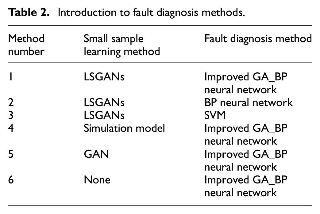
To verify the correctness of the small-sample fault diagnosis model of the high-pressure common rail system established in this research and to compare it with other methods, different diagnostic methods are used for the fault diagnosis of the four operating states mentioned above. The profiles of the different methods are shown in Table 2. Methods one to five are the experimental group, for which the rail pressure signal of state two is generated with different small sample learning methods and fault diagnosis is performed using different fault diagnosis methods. The sixth method is the control group, for which the real rail pressure signal of state two is used for fault diagnosis in order to compare the performance gap between different small sample learning methods and the ideal state.

Table 2.

Introduction to fault diagnosis methods.

Methodnumber	Small samplelearning method	Fault diagnosis method
1	LSGANs	Improved GA_BPneural network
2	LSGANs	BP neural network
3	LSGANs	SVM
4	Simulation model	Improved GA_BPneural network
5	GAN	Improved GA_BPneural network
6	None	Improved GA_BPneural network

To verify the correctness of the fault diagnosis using the simulation model data for small sample learning, a one-dimensional simulation model of the high-pressure common rail system is built using AMESim 13.2, was shown in Figure 15, with the injection sequence A-E-B-C-D. Figure 16 shows the comparison between the experimental and simulation values of the injection pressure under normal conditions. The points where the experimental and simulation curves are poorly matched (such as the data points marked at a, b, c, d, and e in Figure 16) are selected. The simulation values, experimental values, and relative errors of these points are included in Table 3.

Figure 15.

One-dimensional simulation model of high-pressure common rail system.

Figure 16.

Comparison of experimental value and simulation value of fuel injection pressure in state 1.

Table 3.

Comparison table of experimental value and simulation value of fuel injection pressure in state 1.

Datamarkerpoint	Time (ms)	Experimentalvalue(MPa)	Simulationvalue (MPa)	Error(%)
a	3.5	82.233	79.77	2.99
b	3.75	151.51	147.01	2.97
c	4	178.28	171.89	3.58
d	4.25	166.71	162.91	2.27
e	4.5	102.66	101.15	−1.47

From Figure 16 and Table 3, it can be seen that the maximum error between the experimental and simulated values of the injection pressure is within 5%, which meets the simulation requirements. Thus, this simulation model can simulate the operation of this common rail system in the normal state more accurately, and the correctness and the accuracy of the simulation model in the other three states are verified according to the above method. Figures 17 to 19 are graphs showing the comparison of experimental and simulated fuel injection pressure values from state 2 to state 4. The maximum errors are all within 5%. After the above verification, the simulation model is considered to be able to simulate the operation of this five-cylinder diesel engine in the above four states more accurately.

Figure 17.

Comparison of experimental value and simulation value of fuel injection pressure in state 2.

Figure 18.

Comparison of experimental value and simulation value of state 3 fuel injection pressure.

Figure 19.

Comparison of experimental value and simulation value of state 4 fuel injection pressure.

The GAN, simulation model, and LSGANs are used to synthesize 35 sets of rail pressure signals for state two as synthetic data for the training samples. Among the 50 sets of real data for each operation state, 35 sets are randomly selected as training samples, and 3 sets are randomly selected as small sample data in the training samples. The remaining 15 sets are used as test samples, the test samples are numbered sequentially according to the different operation states, and the eigenvectors of the training samples are input into the fault diagnosis model. The 3D eigenvectors of the test samples are input into the fault classifier for fault diagnosis. Table 4 shows the correct rate of each diagnosis and the total correct rate of diagnosis for the different diagnosis methods, Figure 20 shows the diagnosis results of the fault diagnosis using method 1, that is, the method described in this paper. The EMDs in methods 1–5 in the table refer to the average EMD of the synthetic data and the small sample data as training samples, and the EMD in method 6 refers to the average EMD of the real data itself.

Table 4.

Fault diagnosis correct rate of synthetic state 2 rail pressure signals.

Method	Number of diagnosticmodel iterations	EMD (afternormalization)	Status	Number of correctdiagnoses/sample	Diagnosiscorrect rate/%	Total correctrate
1	21	1.91	1	15/15	100	98.3
			2	15/15	100
			3	15/15	100
			4	14/15	93.3
2	44	1.91	1	15/15	100	98.3
			2	15/15	100
			3	15/15	100
			4	14/15	93.3
3	None	1.91	1	15/15	100	86.6
			2	13/15	86.6
			3	13/15	86.6
			4	11/15	73.3
4	24	9.22	1	15/15	100	93.3
			2	12/15	80
			3	15/15	100
			4	14/15	93.3
5	21	1.83	1	15/15	100	96.6
			2	14/15	93.3
			3	15/15	100
			4	14/15	93.3
6	21	1.72	1	15/15	100	98.3
			2	15/15	100
			3	15/15	100
			4	14/15	93.3

Figure 20.

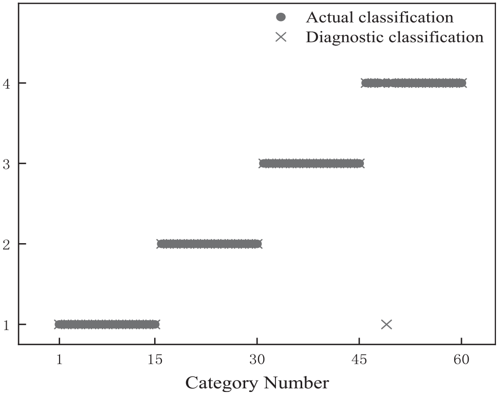
Fault diagnosis results for synthetic state 2 rail pressure signal method 1.

According to the above steps, the rail pressure signals of state 3 and state 4 are synthesized, and the normalized real rail pressure signal and the synthesized rail pressure signal are compared, as shown in Figures 21 and 22.

Figure 21.

Comparison of real rail pressure signal and synthetic rail pressure signal of state 3 after normalization.

Figure 22.

Comparison of real rail pressure signal and synthesized rail pressure signal in state 4 after normalization.

Using the method shown in Table 2, fault diagnosis is performed for state 3 and state 4. For example, Table 5 shows the correct rate of fault diagnosis for the rail pressure signals using different small sample learning methods and fault diagnosis methods for synthesized state 3. Table 6 shows the correct rate of fault diagnosis of the rail pressure signals using different small sample learning methods and fault diagnosis methods for synthesized state 4. Figure 23 shows the fault diagnosis results of method 1 for the synthesized state three rail pressure signals, and Figure 24 shows the fault diagnosis results of method 1 for the synthesized state four rail pressure signals. The EMDs in methods 1–5 in the table refers to the average EMD of the synthetic data and the small sample data used as training samples, and the EMD in method 6 refers to the average EMD of the real data itself.

Table 5.

Fault diagnosis correct rate of synthetic state 3 rail pressure signals.

Method	Number of diagnosticmodel iterations	EMD (afternormalization)	Status	Number of correctdiagnoses/sample	Diagnosiscorrect rate/%	Total correct rate
1	21	1.89	1	15/15	100	98.3
			2	15/15	100
			3	15/15	100
			4	14/15	93.3
2	42	1.89	1	15/15	100	98.3
			2	15/15	100
			3	15/15	100
			4	14/15	93.3
3	None	1.89	1	15/15	100	85
			2	14/15	93.3
			3	11/15	73.3
			4	11/15	73.3
4	23	9.48	1	15/15	100	93.3
			2	15/15	100
			3	12/15	80
			4	14/15	93.3
5	21	1.72	1	15/15	100	98.3
			2	15/15	100
			3	15/15	100
			4	14/15	93.3
6	21	1.64	1	15/15	100	98.3
			2	15/15	100
			3	15/15	100
			4	14/15	93.3

Table 6.

Fault diagnosis correct rate of synthetic state 4 rail pressure signals.

Method	Number of diagnosticmodel iterations	EMD (afternormalization)	Status	Number of correctdiagnoses/sample	Diagnosiscorrect rate/%	Total correct rate
1	21	2.87	1	15/15	100	96.6
			2	15/15	100
			3	15/15	100
			4	13/15	86.6
2	42	2.87	1	15/15	100	96.6
			2	15/15	100
			3	15/15	100
			4	13/15	86.6
3	\	2.87	1	15/15	100	85
			2	14/15	93.3
			3	13/15	86.6
			4	9/15	60
4	24	22.64	1	15/15	100	86.6
			2	15/15	100
			3	15/15	100
			4	7/15	46.6
5	21	1.76	1	15/15	100	91.6
			2	15/15	100
			3	15/15	100
			4	10/15	66.6
6	21	3.11	1	15/15	100	98.3
			2	15/15	100
			3	15/15	100
			4	14/15	93.3

Figure 23.

Fault diagnosis results for the synthetic state 3 rail pressure signal method 1.

Figure 24.

Fault diagnosis results for the synthetic state 4 rail pressure signal method 1.

From the above graphs it can be seen that:

For the small sample learning problem in the fault diagnosis of high-pressure common rail systems, the LSGANs used in this research have the highest correct rate in all fault states, with a correct rate of over 86.6% in the small sample set, indicating that the synthesized rail pressure signals have excellent quality and high diversity. For the case of states 2 and 3, where the average EMD between the real data is small, the correct diagnosis rate for the small sample set can reach 100%. For the case of state 4, where the average EMD between the real data is large, the correct diagnosis rate on the small sample set can still reach 83.3%, when the average EMD between the real data is 3.11, while when using LSGANs, the EMD between the synthesized rail pressure data and the small sample data is 2.87, which is more diverse and can reflect the characteristics of the rail pressure signal in this state. This indicates that this method can synthesize rail pressure data with good quality and diversity in all fault states, and that the method has good generalizability when facing small sample problems. In contrast, the original GAN synthesized rail pressure signals are of high quality and have the smallest average EMD with the real data set in each state, but the diversity is low and the synthesized training samples do not fully reflect the characteristics of the rail pressure signals in this state, although the correct diagnosis rates for the small sample set are 93.3% and 100%, which is not very different from the performance of the LSGANs used in this research. However, in the face of state 4, which is a fault state with a larger average EMD for the real data, the correct diagnosis rate for the small sample set is only 66.6%, and the average EMD for the real data is 3.11 at this time, but the EMD for the rail pressure data synthesized using the original GAN and the small sample data is still 1.76, and the data diversity in this state is poor. This cannot fully reflect the characteristics of the rail pressure signal in this state, and the generalizability is poor. The method of using the simulation model for small sample training achieves the lowest correct rate in several states, and the synthesis quality and diversity are poor, which cannot reflect the characteristics of the rail pressure signal in this state.

The improved GA_BP neural network fault diagnosis model and the BP neural network fault diagnosis model used in this research both have excellent correct diagnosis rates, 98.6%, 98.3%, and 96.6% in the three states. In contrast, the SVM fault diagnosis model has lower correct diagnosis rates, 86.6%, 85%, and 85% in the three states, and the BP neural network is more suitable for solving the fault diagnosis problem of a high-pressure common rail system. However, the improved GA_BP neural network fault diagnosis model requires fewer iterations, requiring an average of 21 generations to complete the training of the neural network, while the traditional BP neural network requires an average of 43 generations. The improved GA_BP neural network used in this research has a faster iteration rate and is more efficient in performing the fault diagnosis of common rail systems.

Based on the above results, it can be concluded that the high-pressure common rail small-sample fault diagnosis method used in this research can solve the problem of small-sample fault diagnosis and generate synthetic data with higher quality, greater diversity, and higher accuracy for fault diagnosis models, as well as having a faster iterative speed, and this method has a higher accuracy rate when facing the problem of the small sample fault diagnosis of a high-pressure common rail in different states.

Conclusion

In this research, we focus on the study of the small-sample fault diagnosis of a high-pressure common rail system. Through a bench test, the rail pressure signals of a high-pressure common rail system with different operating conditions are obtained. By pre-processing the rail pressure signals, high quality rail pressure signals are obtained. To address the current problem of the small sample size of fault signals caused by the difficulty, poor quality, or cost of acquisition, in this research, LSGANs are used to synthesize rail pressure signals, and to obtain a high quality and diverse training sample set. To improve the correct rate of the fault diagnosis model and accelerate the convergence speed of the model, this paper introduces the ART-based initialization population method and the adaptive genetic variation optimization method based on the traditional GA_BP neural network.

In this research, bench test equipment is used to collect pre-processed training and test data, and through the comparison of different combinations of fault diagnosis methods, it is proven that the small sample learning method based on LSGANs has the advantages of high quality and diversity. It is also proven that the fault diagnosis model based on a GA_BP neural network has the advantages of fast convergence and a high correct diagnosis rate. It is verified that the small sample fault diagnosis method used in this research for a high-pressure common rail has excellent diagnostic accuracy for both small-sample faults and other faults. With small-sample learning used to increase the number of training sets, higher signal quality can reduce the number of iterations of the diagnostic model, while higher diversity can characterize the rail pressure signal in this state as much as possible for a limited training set, improving the correct diagnosis rate. Compared with other small-sample learning methods, the LSGANs used in this research have high diversity and high quality in synthesizing rail pressure signals in multiple states, making this the most suitable small-sample learning method for small-sample fault diagnosis in a high-pressure common rail. Compared to other fault diagnosis models, the improved GA_BP neural network used in this research has the highest correct fault diagnosis rate and the fastest iteration speed in the field of common rail system fault diagnosis. The ART initialization population and adaptive genetic mutation optimization optimize the initial value of the BP neural network and increase the iteration speed. The characteristics of the neural network give the neural network a fault diagnosis accuracy rate far exceeding those of other diagnostic models.

Footnotes

Handling Editor: James Baldwin

Declaration of conflicting interests

The author(s) declared no potential conflicts of interest with respect to the research, authorship, and/or publication of this article.

Funding

The author(s) received no financial support for the research, authorship, and/or publication of this article.

ORCID iDs

Liangyu Li

Fukang Ma

References

Fei

Zhang

XB.

Fault diagnosis of power transformer based on support vector machine with genetic algorithm. Expert Syst Appl 2009; 36: 11352–11357.

Wang

Kang

Shen

, et al. Applications of fault diagnosis in rotating machinery by using time series analysis with neural network. Expert Syst Appl 2010; 37: 1696–1702.

Huang

Shen

Long

, et al. The empirical mode decomposition and the Hilbert spectrum for nonlinear and non-stationary time series analysis. Proc Math Phys Eng Sci 1998; 454: 903–995.

Huang

NE.

Ensemble empirical mode decomposition: a noise-assisted data analysis method. Adv Adapt Data Anal 2009; 1: 1–41.

Vapnik

VN.

The nature of statistical learning theory ~. IEEE Trans Neural Netw 1997; 8: 1564–1564.

Widodo

Yang

BS.

Support vector machine in machine condition monitoring and fault diagnosis. Mech Syst Signal Process 2007; 21: 2560–2574.

Huang

Yang

Support vector machine with genetic algorithm for machinery fault diagnosis of high voltage circuit breaker. Measurement 2011; 44: 1018–1027.

Xue

Tan

Shi

, et al. Rope tension fault diagnosis in hoisting systems based on vibration signals using EEMD, improved permutation entropy, and PSO-SVM. Entropy 2020; 22: 209.

Zhou

Zhang

Zhou

, et al. A parameter-adaptive variational mode decomposition approach based on weighted fuzzy-distribution entropy for noise source separation. Meas Sci Technol 2020; 31: 125004.

10.

Qiao

, et al. Misfire fault diagnosis method for diesel engine based on MEMD and dispersion entropy. Shock Vib 2021; 2021: 1–14.

11.

Zhao

Mao

Zhang

, et al. Multi-branch convolutional neural networks with integrated cross-entropy for fault diagnosis in diesel engines. Meas Sci Technol 2021; 32: 045103.

12.

Kumar

Gandhi

Zhou

, et al. Improved CNN for the diagnosis of engine defects of 2-wheeler vehicle using wavelet synchro-squeezed transform (WSST). Knowl Based Syst 2020; 208: 1122–1134.

13.

Torres

Colominas

Schlotthauer

, et al. A complete ensem ble empirical mode decomposition with adaptive noise. In: Proceedings of IEEE conference on acoustics, speech and signal processing, Prague, Czech Republic, 22–27 May 2011, pp.4144–4147.

14.

Dragomiretskiy

Zosso

Veriational mode decomposition. IEEE Trans Signal Process 2014; 62: 531–544.

15.

Aneesh

Kumar

Hisham

, et al. Performance comparison of variational mode decomposition over empirical wavelet transform for the classification of power quality disturbances using support vector machine. Procedia Comput Sci 2015; 46: 372–380.

16.

Huang

GB.

Extreme learning machine for regression and multiclass classification. IEEE Trans Syst Man Cybern 2012; 42: 513–529.

17.

Lei

Lin

, et al. A review on empirical mode decomposition in fault diagnosis of rotating machinery. Mech Syst Signal Process 2013; 35: 108–126.

18.

Rai

Upadhyay

SH.

An integrated approach to bearing prognostics based on EEMD-multi feature extraction, Gaussian mixture models and Jensen-Rényi divergence. Appl Soft Comput 2018; 71: 36–50.

19.

Jegadeeshwaran

Sugumaran

Fault diagnosis of automobile hydraulic brake system using statistical features and support vector machines. Mech Syst Signal Process 2015; 52-53: 436–446.

20.

Long

Zhu

Survey of few-shot learning based on deep neural network. Appl Res Comput 2020; 37: 2241–2247.

21.

Jankowski

Duch

Grąbczewski

Meta-learning in computational intelligence. 4th ed. Berlin: Springer Science and Business Media, 2011, p.97.

22.

Fei-Fei

Fergus

Perona

One-shot learning of object categories. IEEE Trans Pattern Anal Mach Intell 2006; 28: 594–611.

23.

Xiang

Jiang

, et al. Recent advances in zero-shot recognition: toward data-efficient understanding of visual content. IEEE Signal Process Mag 2018; 35: 112–125.

24.

Yang

Liu

YL.

The latest advances in face recognition with single training sample. J Xihua Univ 2014; 33: 1–10.

25.

Zhong

Xingliang

Chai

Yunlong

. Improved prototypical networks for few-Shot learning. Pattern Recognition Letters 2020; 140: 81–87.

26.

Kailin

Jin

Wang

A review of small sample learning research. J Softw 2021; 32: 349–369.

27.

Royle

Dorazio

Link

WA.

Analysis of multinomial models with unknown index using data augmentation. J Comput Graph Stat 2007; 16: 67–85.

28.

Radford

Metz

Chintala

Unsupervised representationlearning with deep convolutional generative adversarial networks. arXiv preprint arXiv:1511.06434, 2015.

29.

Silver

Schrittwieser

Simonyan

, et al. Mastering the game of go without human knowledge. Nature 2017; 550: 354–359.

30.

Ulyanov

Vedaldi

Lempitsky

Instance normalization:the missing ingredient for fast stylization. Online Referencing, 2(3). https://arxiv.org/pdf/1607.08022.Pdf (2016, accessed 13 February 2020).

31.

Wang

Zhang

Van De

Weijer J.

Ensembles of gener-ative adversarial networks. arXiv preprint arXiv:1612.00991, 2016.

32.

Mao

Xie

, et al. On the effectiveness of least squares generative adversarial networks. IEEE Trans Pattern Anal Mach Intell 2019; 41: 2947–2960.

33.

Cheng

Dai

, et al. Prediction of facial deformation after complete denture prosthesis using BP neural network. Comput Biol Med 2015; 66: 103–112.

34.

Suganthi

Natarajan

Sathiyamurthy

, et al. Prediction of quality responses in micro-EDM process using an adaptive neuro-fuzzy inference system(ANFIS) model. Int J Adv Manuf Technol 2013; 68: 339–347.

35.

Oreski

Genetic algorithm-based heuristic for feature selection in credit risk assessment. Expert Syst Appl 2014; 41: 2052–2064.

36.

Sohail

Noor

Farwa

, et al. Neural network forecasting of the flow regimens of viscous fluids in a 3D reactor. Adv Mech Eng 2021; 13: 168781402199952.

37.

Svorcan

Peković

Simonović

, et al. Design of optimal flow concentrator for vertical-axis wind turbines using computational fluid dynamics, artificial neural networks and genetic algorithm. Adv Mech Eng 2021; 13: 16878140211009009.

38.

Siqi

Wang

Yufang

Low-dose CT denoising algorithm based on improved cyclic consistency generation adversarial network. Acta Opt Sin 2020; 40: 70–78.

39.

Sun

HQ.

Fractal geometry and fractal interpolation. 4th ed. Beijing: Science Press, 2011, p.99.

40.

Rubner

Tomasi

Guibas

LJ.

The earth mover’s distance as a metric for image retrieval. Int J Comput Vis 2000; 40: 99–121.

41.

Nikravan

Parsa

Hybrid adaptive random testing. Int J Comput Sci Math 2020; 11: 209–258.

Research on a small sample fault diagnosis method for a high-pressure common rail system

Abstract

Keywords

Introduction

Extraction and pre-processing of rail pressure signal

LSGAN-based rail pressure data synthesis

Common rail system fault diagnosis model

EEMD-based rail pressure signal decomposition and eigenvalue extraction

Improved GA_BP neural network fault diagnosis model

Experiments and results analysis

Conclusion

Footnotes

Declaration of conflicting interests

Funding

ORCID iDs

References