Trajectory tracking control for four-wheel independent drive intelligent vehicle based on model predictive control and sliding mode control

Abstract

For four-wheel independent drive intelligent vehicle, the longitudinal and lateral motion control of the vehicle is decoupled and a hierarchical controller is designed: the upper layer is the motion controller, and the lower layer is the control distributor. In the motion controller, the model predictive control (MPC) is used to calculate the steering wheel angle and the total yaw moment for lateral control, and the sliding mode control (SMC) is used to calculate the total driving force for longitudinal control. In order to improve the control algorithm adaptability and the tracking accuracy at high speed, the UniTire model that can accurately express the complex coupling characteristics of tire under different working conditions are used and the numerical partial derivative of the state equation is used in MPC controller to ensure the feasibility of the algorithm. The control distributor distributes the total yaw moment and driving force calculated by the motion controller of the four wheels through the objective optimization function, and the constraints on road adhesion condition and the constraints on actuators are considered at the same time. A co-simulation platform is built in the CarSim/Simulink environment and the MPC-SMC controller is compared with the previously established MPC controller.

Introduction

Traditional vehicles are driven by drivers and their personal factors are the main cause of various traffic accidents. Traditional vehicle emissions can also cause environmental pollution. ¹ However, the intelligence of automobiles can solve this problem well. They can be widely used in transportation, agriculture, planetary exploration, military, and other aspects. Distributed drive electric vehicles have become the focus on current automotive research due to the advantages of low noise, no emissions, simple chassis structure, independent control of the four-wheel driving/braking torque, and high energy transmission efficiency. ²

Scholars have proposed many control methods of the trajectory tracking of intelligent vehicles. MacAdam^3,4 considered the driver’s forward-looking characteristics and applied the preview optimal control to the driver model based on a small heading angle. On the basis of the preview optimal driver model, Guo and Guan ⁵ established the preview optimal curvature driver model. In 2002, a preview-optimized artificial neural network driver model (POSANN) was proposed and the front wheel steering angle was decided based on the preview point and the current vehicle state. Analytical values of model parameters can be obtained by error analysis. ⁶ Soudbakhsh and Eskandarian ⁷ designed two SMC trajectory tracking controllers with linear tire model and compared them with LQR controller at different speeds. The results showed that the SMC controller was better in yaw angle control. Wu and Si ⁸ realized trajectory tracking control based on the linear matrix inequality. The saturated linear tire was used to obtain the vehicle lateral dynamic multi-cell model including the time-varying characteristics of the tire and the designed controller was compared with the model prediction controller and the preview driver model. The results showed that the controller had better tracking accuracy. A composite control method combining MPC and adaptive fuzzy control is proposed, which realizes the trajectory tracking control of the tractor in a complex environment. ⁹ Zhang et al. ¹⁰ proposed a robust control scheme that combines backstepping method, neural network, and SMC to achieve underactuated vehicle trajectory tracking under parameter uncertainty and external interference. Shuo Zhang et al. ¹ proposed a preview controller based on adaptive SMC and a feedback controller based on fuzzy control. The extension theory is introduced to adjust the control ratio of the two controllers, which improves the adaptability and robustness of the algorithm. Chen et al. ¹¹ adopted the supertwist second-order sliding mode to suppress the chattering issue and proposed a nonlinear disturbance observer to improve the robustness of the system to disturbances, which realize the trajectory tracking of four-wheel independent driving electric vehicles. The performance of the controller is better than PID control and first-order SMC. Fei et al. ¹² designed a fuzzy double hidden layer recurrent neural network controller for a class of nonlinear systems using a terminal sliding-mode control, which increase the dynamic approximation ability and reduce the switching gain.

Model predictive control has been widely used because of its robustness and its ability to handle multi constraints and multi coupling problems. Yoon et al. ¹³ used a hyperbolic tangent function to approximate the magic formula and the NMPC controller was designed to control the autonomous ground vehicle longitudinally and laterally and avoid obstacle based on the tire model. Zhou et al. ² used the Burckhardt tire model to build a seven-DOF (degrees of freedom) nonlinear vehicle model and used NMPC to design a longitudinal and lateral coordinated controller for four-wheel independent drive electric vehicles to track the desired yaw rate and vehicle speed. The effectiveness of the controller was verified by the HIL test platform and it had strong robustness to the road adhesion coefficient. Choi and Kang ¹⁴ used NMPC-based active steering and braking to increase the current operating range of the Autonomous Emergency Braking (AEB) system. The front wheels steering angle and longitudinal acceleration were the control variables to minimize the deviation between the predicted vehicle trajectory and the expected trajectory and the steering angle was constrained to ensure the stability of the vehicle. Kong et al. ¹⁵ studied the application of the linear two-DOF vehicle model and kinematic models in autonomous driving. Based on the experimental data, the author discussed the errors caused by the two models in predicting the state of the vehicle and analyzed the effect of discretization on the prediction error. The MPC controller was designed with the kinematic model and the effectiveness of the controller was verified under windy environments and different vehicle speeds. There are also some scholars that studied the trajectory tracking of vehicles for low road adhesion and the use of model predictive control can make vehicles have higher tracking accuracy while ensuring stability.^16–18 Zhang et al. ¹⁹ proposed an adaptive learning MPC for the trajectory tracking of input constrained vehicles subject to parametric uncertainties and additive disturbances and guaranteed the recursive feasibility and closed-loop stability. The results show that the tracking accuracy of the designed controller is better than robust MPC. In addition, MPC control can also realize simultaneous vehicle trajectory planning and tracking. Guo et al. ²⁰ realized the obstacle avoidance trajectory planning and tracking of the vehicle based on MPC control by establishing a single-track model and measuring the yaw angle, velocity, and angular velocity of the obstacle vehicle.

The local linearization of the nonlinear vehicle dynamic model with PAC tire model have been adopted by the author to design the MPC trajectory tracking controller, which is superior to the PDM controller of trajectory tracking accuracy and maintaining vehicle stability. However, the control objective of the MPC controller is to minimize the objective function by the method of weighting. The objective function consider the weighting of the control variable, control increment, control output, and relaxation factor, resulting in a certain error between the control output and the reference value. ²¹ Trajectory tracking requires not only the tracking of the position, but also the tracking of the speed. In order to reduce the vehicle speed tracking error, the longitudinal and lateral motion control of the vehicle are decoupled and a hierarchical controller is designed.

One of the innovations in this article is to decouple the longitudinal and lateral motion control of the vehicle. The coupling characteristics of tire mechanics based on UniTire model ²² are considered in the longitudinal and lateral stability constraints. The results show that the designed controller is superior to the traditional MPC controller of speed control. The second innovation in this paper is the use of the UniTire model that can accurately express the complex coupling characteristics of tire under different working conditions. Because of its dimensionless force characteristic expression, plug-in friction coefficient, theoretical model boundary conditions, and other modeling characteristics, UniTire model not only has high model accuracy, but also owns a good model expansion capabilities. In the control system of this article, the nonlinearity of the system is treated with local linearization. Using the complicated UniTire model, a simple numerical calculation method is developed to approximate the partial derivative of the tire force with respect to the state quantity, avoiding complicated formulas derivation, and complex numerical solution of control algorithm. The use of high-precision tire model makes the algorithm more extensible and can also improve the tracking accuracy under extreme conditions.

The contents of the rest sections are as follows. In section 2, the 7-degrees of freedom vehicle model and the UniTire model used in the controller are established. The parameterized vehicle model in Carsim is established as the controlled plant. According to the real vehicle experimental data, the accuracy of the Carsim model is verified. In Section 3, the hierarchical controller is designed, in which the upper layer is the motion controller and the lower layer is the control distributor. In the motion controller, the model predictive control is used to calculate the steering wheel angle and total yaw moment for lateral control. The sliding mode control is applied to calculate the total driving force for longitudinal control. And the control distributor optimally distributes the total yaw moment and driving force to the four wheels. In section 4, the trajectory tracking performance of different tire models and control methods is compared. Conclusions are achieved in Section 5.

System model

Vehicle dynamic model

In order to reduce the complexity of the algorithm, the vehicle model is simplified. For vehicle control system development, the seven-degrees of freedom model is a classic and often used vehicle reference model.^2,21,23,24 Among different vehicle models, the most important and main difference is that different tire models are used. This paper uses UniTire model that can accurately express the complex coupling characteristics of tire under different working conditions. ²⁵ The longitudinal movement, lateral movement, and yaw movement of the vehicle is controlled in trajectory tracking, so their characteristics need to be analyzed.

According to the theory of automotive dynamics, the motion equations of the vehicle center of gravity (CG) along the X-axis, Y-axis, and around the Z-axis of the vehicle coordinate system can be obtained, at the meantime the rotation of the wheels is considered. The nonlinear dynamic model of the vehicle is established. ²¹

Longitudinal motion:

$$\begin{array}{c}\multicolumn{1}{c}{m({\stackrel{·}{V}}_x-\stackrel{·}{\phi }{V}_y)=(F_{x1}+F_{x2})\cos \delta -(F_{y1}+F_{y2})\sin \delta }\\ \multicolumn{1}{c}{+F_{x3}+F_{x4}}\end{array}$$

(1)

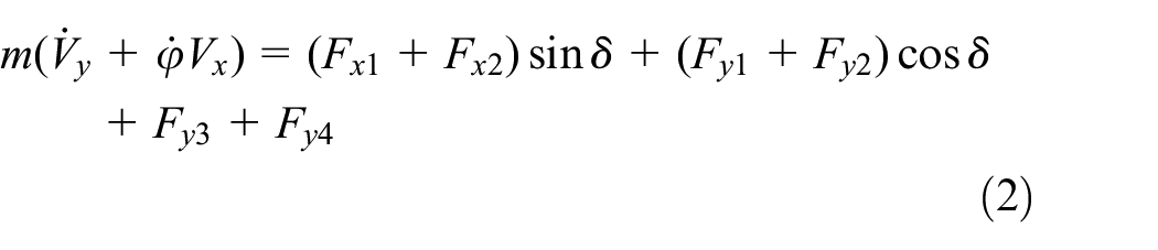
Lateral motion:

$$\begin{array}{c}\multicolumn{1}{c}{m({\stackrel{·}{V}}_y+\stackrel{·}{\phi }{V}_x)=(F_{x1}+F_{x2})\sin \delta +(F_{y1}+F_{y2})\cos \delta }\\ \multicolumn{1}{c}{+F_{y3}+F_{y4}}\end{array}$$

(2)

Yaw motion:

$$\begin{array}{c}\multicolumn{1}{c}{J_Z\stackrel{··}{\phi }=l_a(F_{x1}+F_{x2})\sin \delta +l_a(F_{y1}+F_{y2})\cos \delta }\\ \multicolumn{1}{c}{-l_b(F_{y3}+F_{y4})}\\ +\frac{c}{2}(F_{x2}-F_{x1})\cos \delta +\frac{c}{2}(F_{x4}-F_{x3})\hfill \\ \multicolumn{1}{c}{+\frac{c}{2}(F_{y1}-F_{y2})\sin \delta }\end{array}$$

(3)

Wheels rotation:

$$J_{\omega i}{\stackrel{·}{\omega }}_i=T_i-R_{\mathrm{ei}}{F}_{\mathrm{xi}}-B_i{\omega }_i$$

(4)

where m is the vehicle mass. J_Z is the yaw inertia. F_xi and F_yi is the longitudinal and lateral tire forces respectively. The nonlinear characteristics of the vehicle are largely determined by the tire properties. V_x and V_y are the longitudinal and lateral speed relative to the vehicle coordinate system. $\stackrel{·}{\phi }$ is the yaw rate. $\delta$ is the front wheel steering angle. c is the wheel track. l_a and l_b are distances from CG to front and rear axle respectively. T_i is the torque on each wheel. $J_{\omega i}$ is the wheel rotational inertia. R_ei is the wheel effective rolling radius. ${\omega }_i$ is the wheel angular speed. B_i is the viscous resistance coefficient. i = 1, 2, 3, 4 indicates front left, front right, rear left, and rear right wheel respectively. Figure 1 depicts the diagram of seven-DOF vehicle dynamic model.

Figure 1.

Seven-DOF vehicle dynamic model.

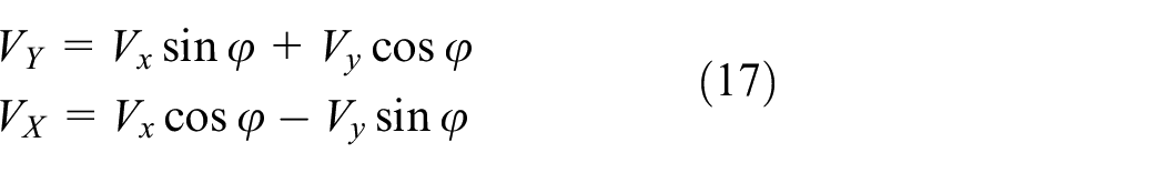
The speed of the vehicle center of mass relative to the inertial coordinates system is:

$$\begin{array}{c}{V}_Y=V_x\sin \phi +V_y\cos \phi \hfill \\ V_X=V_x\cos \phi -V_y\sin \phi \hfill \end{array}$$

(5)

The input of the UniTire model includes longitudinal slip ratio, side slip angle, vertical load, speed of wheel center, camber angle, turn-slip properties. The turn-slip properties are usually considered when the vehicle has large steer angle at low speed. UniTire adopts the expression of dynamic friction coefficient. It is different from the adhesion coefficient, but establishes a functional relationship between the friction coefficient and the tire slip rate. Because of the small camber angle of modern vehicles, after ignoring the influence of camber angle, the UniTire model can be expressed as the following function:

$$\begin{array}{c}{F}_{\mathrm{xi}}=f({\alpha }_i,{\kappa }_i,v_i,F_{\mathrm{z}i})\hfill \\ F_{\mathrm{yi}}=f({\alpha }_i,{\kappa }_i,v_i,F_{\mathrm{z}i})\hfill \end{array}$$

(6)

where ${\alpha }_i$ is the side slip angle. ${\kappa }_i$ is the longitudinal slip ratio. $v_i$ is the speed of wheel center. $F_{\mathrm{zi}}$ is the vertical load on the tire.

The static load of the tire is only affected by the center of mass in the steady state and the dynamic load is caused by the pitch and roll of the vehicle when the vehicle is running. Although the pitch and roll motion of the vehicle are ignored in this paper, the longitudinal/lateral acceleration of the vehicle will also cause the vertical load of the tire to change. Therefore, the vertical load can be expressed as (7) ²¹ :

$$\begin{array}{c}{F}_{z1}=\mathrm{mg}\frac{l_b}{2L}-m{a}_x\frac{H}{2L}-m{a}_y\frac{l_{b}H}{\mathrm{Lc}}+m{a}_x{a}_y\frac{H^2}{\mathrm{gLc}}\hfill \\ F_{z2}=\mathrm{mg}\frac{l_b}{2L}-m{a}_x\frac{H}{2L}+m{a}_y\frac{l_{b}H}{\mathrm{Lc}}-m{a}_x{a}_y\frac{H^2}{\mathrm{gLc}}\hfill \\ F_{z3}=\mathrm{mg}\frac{l_a}{2L}+m{a}_x\frac{H}{2L}-m{a}_y\frac{l_{a}H}{\mathrm{Lc}}-m{a}_x{a}_y\frac{H^2}{\mathrm{gLc}}\hfill \\ F_{z4}=\mathrm{mg}\frac{l_a}{2L}+m{a}_x\frac{H}{2L}+m{a}_y\frac{l_{a}H}{\mathrm{Lc}}+m{a}_x{a}_y\frac{H^2}{\mathrm{gLc}}\hfill \end{array}$$

(7)

where H is the height of CG. L is the wheelbase.

The side slip angles are as formula (8):

$$\begin{array}{c}{\alpha }_1=\arctan [(V_y+l_a\stackrel{·}{\phi })/(V_x-\frac{c}{2}\stackrel{·}{\phi })]-\delta \hfill \\ {\alpha }_2=\arctan [(V_y+l_a\stackrel{·}{\phi })/(V_x+\frac{c}{2}\stackrel{·}{\phi })]-\delta \hfill \\ {\alpha }_3=\arctan [(V_y-l_a\stackrel{·}{\phi })/(V_x-\frac{c}{2}\stackrel{·}{\phi })]\hfill \\ {\alpha }_4=\arctan [(V_y-l_a\stackrel{·}{\phi })/(V_x+\frac{c}{2}\stackrel{·}{\phi })]\hfill \end{array}$$

(8)

Tire model

The vehicle control system requires complex numerical calculations, so the simplified tire model with fewer parameters is often used in the reference vehicle model. Even if more complicated tire model is applied, such as magic formulas, the mechanical characteristics of the combined operating conditions are still achieved by simplification processing of pure operating conditions properties.^23,24 The error caused by the simplification of tire characteristics depends on the robustness of the control system to compensate. The feature of this paper is to directly apply the complicated UniTire model proposed by Konghui Guo.

The longitudinal and lateral slip ratios $S_x$ and $S_y$ can all be defined in the unified form:

$$\begin{array}{c}{S}_x=\frac{-V_{\mathrm{sx}}}{\omega R_e},\kappa =\frac{S_x}{1-S_x}\hfill \\ S_y=\frac{-V_{\mathrm{sy}}}{\omega R_e}\hfill \\ S_x,S_y\in (-\infty ,+\infty )\hfill \end{array}$$

(9)

$${\varphi }_x=\frac{K_x{S}_x}{F_{\mathrm{xm}}},{\varphi }_y=\frac{K_y{S}_y}{F_{\mathrm{ym}}},\varphi =\sqrt{{\varphi }_x^2+{\varphi }_y^2}$$

(10)

$$F_{\mathrm{xm}}={\mu }_x{F}_z,F_{\mathrm{ym}}={\mu }_y{F}_z$$

(11)

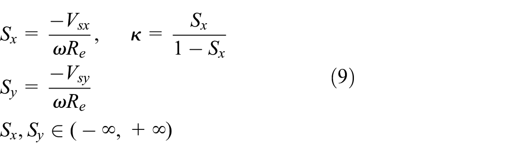
where R_e is the effective rolling radius. V_sx and V_sy are the relative sliding speeds in the contact patch with respect to the road surface. K_x and K_y are longitudinal sliding stiffness and lateral stiffness. ${\varphi }_x$ , ${\varphi }_y$ , and $\varphi$ are the normalized longitudinal, lateral, and combined slip ratios.

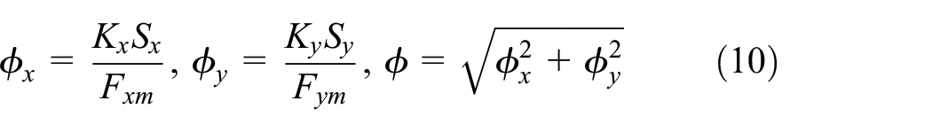
Dynamic friction coefficients are as formula (12):

$$\begin{array}{c}{\mu }_x={\mu }_{\mathrm{xs}}+({\mu }_{\mathrm{xm}}-{\mu }_{\mathrm{xs}})·\hfill \\ \exp (-{\mu }_{\mathrm{xh}}^2{\log }^2(\left|\frac{V_{\mathrm{sx}}}{V_{\mathrm{sxm}}}\right|+\exp (-\left|\frac{V_{\mathrm{sx}}}{V_{\mathrm{sxm}}}\right|)))\hfill \\ {\mu }_y={\mu }_{\mathrm{ys}}+({\mu }_{\mathrm{ym}}-{\mu }_{\mathrm{ys}})·\hfill \\ \exp (-{\mu }_{\mathrm{yh}}^2{\log }^2(\left|\frac{V_{\mathrm{sy}}}{V_{\mathrm{sym}}}\right|+\exp (-\left|\frac{V_{\mathrm{sy}}}{V_{\mathrm{sym}}}\right|)))\hfill \end{array}$$

(12)

where ${\mu }_{\mathrm{xs}}$ , ${\mu }_{\mathrm{ys}}$ , ${\mu }_{\mathrm{xm}}$ , ${\mu }_{\mathrm{ym}}$ , ${\mu }_{\mathrm{xh}}$ , ${\mu }_{\mathrm{yh}}$ , $V_{\mathrm{sxm}}$ , and $V_{\mathrm{sym}}$ are the friction characteristic parameters.

The longitudinal and lateral forces can be expressed as:

$$\{\begin{array}{c}\overline{F}=1-\exp (-\varphi -E_1{\varphi }^2-(E_1^2+\frac{1}{12}){\varphi }^3)\hfill \\ \multicolumn{1}{c}{F_x=\overline{F_x}{\mu }_x{F}_z}\\ \multicolumn{1}{c}{F_y=\overline{F_y}{\mu }_y{F}_z}\end{array}$$

(13)

$$\begin{array}{c}\overline{F_x}=\overline{F}\frac{\lambda {\varphi }_x}{\sqrt{{\left(\lambda {\varphi }_x\right)}^2+{\varphi }_y^2}}\hfill \\ \overline{F_y}=\overline{F}\frac{\lambda {\varphi }_y}{\sqrt{{\left(\lambda {\varphi }_x\right)}^2+{\varphi }_y^2}}\hfill \end{array}$$

(14)

where $\overline{F_x}$ , $\overline{F_y}$ , and $\overline{F}$ is the normalized longitudinal, lateral, and total shear force. $E_1$ is curvature factor. $\lambda$ is the modification factor. ²⁵

Based on tire mechanical property experimental data, the UniTire model parameters are solved by nonlinear least squares fitting. The comparison of model simulation and test data under different vertical loads (2000, 4000, 6000 N) are shown in Figure 2. In view of UniTire based on physical model, adopting unified normalized slip ratios and forces, and the structure of the inserted friction coefficient, it has better multi-conditions transplantation, and it is convenient to apply to different running conditions from the test conditions.

Figure 2.

Tire model parameter identification result: (a) longitudinal forces under pure longitudinal slip conditions, (b) lateral forces under pure side slip conditions, (c) longitudinal forces under the combined slip conditions, and (d) lateral forces under the combined slip conditions.

Carsim vehicle model

The main parameters of the whole vehicle are shown in Table 1 and the characteristic curves of the suspension components are shown in Appendix A. The CarSim model includes vehicle body, tires, steering system, suspension system, etc. Parameter measurement and performance tests are performed on the sub-systems of the controlled vehicle. ²⁶ The relevant data is filled into the parameterized interface. In the CarSim vehicle model, the Pacejka 5.2 tire model embedded in the software is used. Appendix B shows the model parameter setting interface and the corresponding parameter values. The model parameters come from the fitting of the multi-condition tire test data. The detailed discussion of the model can refer to Professor Pacejka’s ²⁷ monograph on tire dynamics. In order to verify the parameterized model, the snake test and steering angle step test of 70 km/h were implemented. The measured speed and steering angle of the real vehicle are used as the input of the Carsim model. The yaw rate and lateral acceleration of the simulation and test results are compared. The comparison results are shown in Figure 3. The steering controller in Carsim adopts the optimal control theory proposed by MacAdam,^3,4 which has been streamlined and re-formulated. Based on the square deviation of the preview point and the reference trajectory, a quadratic performance index is defined to solve the optimal control value. The task performed by the steering controller is to calculate a new value of steering angle at the front wheels as the simulation proceeds, using the preview target location. Solvers in Carsim use PID control to simulate the effect of a driver attempting to maintain a target speed.

Table 1.

The main parameters of the whole vehicle.

Parameter name	Value
Mass of the whole vehicle/kg	1629.56
Height of CG (center of gravity)/mm	633.34
Unsprung mass/kg	182
Roll inertia (Ixx)/kg m2	732.2
Roll inertia (Iyy)/kg m2	2596.8
Roll inertia (Izz)/kg m2	2814.2
Product (Ixy)/kg m2	34.4
Product (Ixz)/kg m2	−81.8
Product (Iyz)/kg m2	26.1
The front axle distance to CG/mm	1212.69
The rear axle distance to CG/mm	1538.66
Track width/mm	1556.67

Figure 3.

Carsim vehicle model verification: (a) lateral acceleration of snake test, (b) yaw rate of snake test, (c) lateral acceleration of steering angle step test, and (d) yaw rate of steering angle step test.

Design of hierarchical controller

MPC controller

Figure 4 depicts the structure of the trajectory tracking controllers. Considering that the driving force/braking force of the four wheels can be controlled independently, the term containing the longitudinal force in the yaw motion equation is replaced by a total yaw moment. The horizontal component of the longitudinal force is small and can be regarded as a disturbance term in lateral motion. Therefore, the longitudinal force within the predictive horizon domain can be approximated as a constant. The vehicle system dynamic equations are established as formula (15):

Figure 4.

The structure of the controller: (a) MPC controller and (b) MPC-SMC controller.

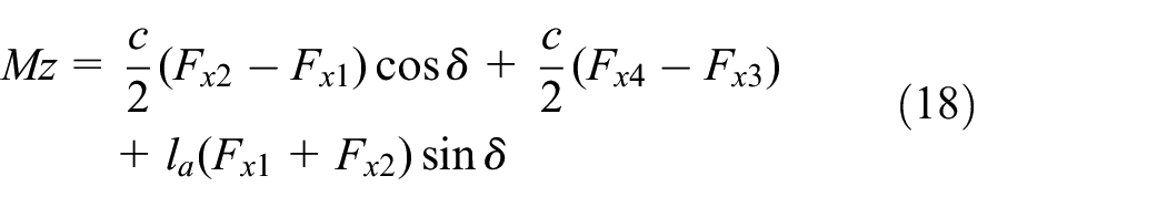
Yaw motion:

$$\begin{array}{c}{J}_Z\stackrel{··}{\phi }=l_a(F_{y1}+F_{y2})\cos \delta -l_b(F_{y3}+F_{y4})\hfill \\ +\frac{c}{2}(F_{y1}-F_{y2})\sin \delta +\mathrm{Mz}\hfill \end{array}$$

(15)

Lateral motion:

$$\begin{array}{c}m({\stackrel{·}{V}}_y+\stackrel{·}{\phi }{V}_x)=(F_{x1}+F_{x2})\sin \delta +\hfill \\ (F_{y1}+F_{y2})\cos \delta +F_{y3}+F_{y4}\hfill \end{array}$$

(16)

The speed of the vehicle center of mass relative to the inertial coordinate system is:

$$\begin{array}{c}{V}_Y=V_x\sin \phi +V_y\cos \phi \hfill \\ V_X=V_x\cos \phi -V_y\sin \phi \hfill \end{array}$$

(17)

where

$$\begin{array}{c}\multicolumn{1}{c}{\mathrm{Mz}=\frac{c}{2}(F_{x2}-F_{x1})\cos \delta +\frac{c}{2}(F_{x4}-F_{x3})}\\ +l_a(F_{x1}+F_{x2})\sin \delta \hfill \end{array}$$

(18)

The lateral motion, yaw motion, and location relative to the inertial coordinate system are considered in the lateral model predictive controller. The following five variables are considered as the state variables of the controller:

$$\mathit{\xi }={\left[V_{\mathrm{y}}\phi \stackrel{·}{\phi }\right]}^T$$

(19)

The total yaw moment and the steering angle are defined as control variables:

$$\mathit{\mu }={\left[\mathrm{Mz}\delta \right]}^T$$

(20)

In order to track the desired path accurately, $\phi$ and Y are selected as the control output variables. In order to ensure the stability of the controller, four tire side slip angles are constrained:

$$\mathit{\eta }={\left[\phi {\alpha }_1{\alpha }_2{\alpha }_3{\alpha }_4\right]}^T$$

(21)

The nonlinear vehicle dynamic model is as following:

$$\begin{array}{c}\stackrel{·}{\mathit{\xi }}=\mathit{f}(\mathit{\xi },\mathit{\mu })=\left[\begin{array}{c}{f}_1(\mathit{\xi },\mathit{\mu })\hfill \\ \multicolumn{1}{c}{f_2(\mathit{\xi },\mathit{\mu })}\\ \multicolumn{1}{c}{f_3(\mathit{\xi },\mathit{\mu })}\\ \multicolumn{1}{c}{f_4(\mathit{\xi },\mathit{\mu })}\\ \multicolumn{1}{c}{f_5(\mathit{\xi },\mathit{\mu })}\end{array}\right]\hfill \\ \mathit{\eta }=\mathit{h}(\mathit{\xi },\mathit{\mu })={\left[\phi {\alpha }_1{\alpha }_2{\alpha }_3{\alpha }_4\right]}^T\hfill \end{array}$$

(22)

where

$$\{\begin{array}{c}{f}_1(\mathit{\xi },\mathit{\mu })=\left(\begin{array}{c}(F_{x1}+F_{x2})\sin \delta +(F_{y1}+F_{y2})\cos \delta \hfill \\ \multicolumn{1}{c}{+F_{y3}+F_{y4}}\end{array}\right)/m-\stackrel{·}{\phi }{V}_x\hfill \\ \multicolumn{1}{c}{f_2(\mathit{\xi },\mathit{\mu })=\stackrel{·}{\phi }}\\ \multicolumn{1}{c}{f_3(\mathit{\xi },\mathit{\mu })=\left(\begin{array}{c}{l}_a(F_{y1}+F_{y2})\cos \delta -l_b(F_{y3}+F_{y4})\hfill \\ \multicolumn{1}{c}{+\frac{c}{2}(F_{y3}-F_{y4})\sin \delta +\mathrm{Mz}}\end{array}\right)/J_{\mathrm{Z}}}\\ \multicolumn{1}{c}{f_4(\mathit{\xi },\mathit{\mu })=V_x\sin \phi +V_y\cos \phi }\\ \multicolumn{1}{c}{f_5(\mathit{\xi },\mathit{\mu })=V_x\cos \phi -V_y\sin \phi }\end{array}$$

$$\{\begin{array}{c}{\mathit{h}}_1(\mathit{\xi },\mathit{\mu })=\phi \hfill \\ \multicolumn{1}{c}{{\mathit{h}}_2(\mathit{\xi },\mathit{\mu })=Y}\\ \multicolumn{1}{c}{{\mathit{h}}_3(\mathit{\xi },\mathit{\mu })=\arctan [(V_y+l_a\stackrel{·}{\phi })/(V_x-\frac{c}{2}\stackrel{·}{\phi })]-\delta }\\ \multicolumn{1}{c}{{\mathit{h}}_4(\mathit{\xi },\mathit{\mu })=\arctan [(V_y+l_a\stackrel{·}{\phi })/(V_x+\frac{c}{2}\stackrel{·}{\phi })]-\delta }\\ \multicolumn{1}{c}{{\mathit{h}}_5(\mathit{\xi },\mathit{\mu })=\arctan [(V_y-l_a\stackrel{·}{\phi })/(V_x-\frac{c}{2}\stackrel{·}{\phi })]}\\ \multicolumn{1}{c}{{\mathit{h}}_6(\mathit{\xi },\mathit{\mu })=\arctan [(V_y-l_a\stackrel{·}{\phi })/(V_x+\frac{c}{2}\stackrel{·}{\phi })]}\end{array}$$

The theoretical derivation of the linear time-varying model predictive controller ²⁰ has been realized in the previous work. In the discrete linear time-varying system, A_t and B_t are the Jacobian matrix of the state equation relative to the state quantity and the control quantity obtained by the partial derivative rule, as equation (23). However, considering the complexity of UniTire model, if A_t and B_t are still solved by the analytical method, its result will be too complicated to run the algorithm. On the other hand, UniTire is a semi-empirical tire model, which contains empirical expressions to adapt to the test data, and a completely mathematical analytical deviation may lead to incorrect results.

So in the control system, numerical approximations ${\hat{\mathit{A}}}_t$ and ${\hat{\mathit{B}}}_t$ are used as (24).

$$\begin{array}{c}{\mathit{A}}_t={\frac{\partial \mathit{f}(\mathit{\xi }(t),\mathit{\mu }(t))}{\partial \mathit{\xi }}|}_{\mathit{\xi }(t),\mathit{\mu }(t-1)}\hfill \\ {\mathit{B}}_t={\frac{\partial \mathit{f}(\mathit{\xi }(t),\mathit{\mu }(t))}{\partial \mathit{\mu }}|}_{\mathit{\xi }(t),\mathit{\mu }(t-1)}\hfill \end{array}$$

(23)

$$\begin{array}{c}{\hat{\mathit{A}}}_t=\frac{\mathit{f}(\mathit{\xi }(t),\mathit{\mu }(t))-\mathit{f}(\mathit{\xi }(t-1),\mathit{\mu }(t))}{\mathit{\xi }\left(t\right)-\mathit{\xi }(t-1)}\hfill \\ {\hat{\mathit{B}}}_t=\frac{\mathit{f}(\mathit{\xi }(t),\mathit{\mu }(t))-\mathit{f}(\mathit{\xi }(t),\mathit{\mu }(t-1))}{\mathit{\mu }(t)-\mathit{\mu }(t-1)}\hfill \end{array}$$

(24)

In the tracking control, the simulation step length is usually set short enough, so this method will not lead to a significant decrease in tracking accuracy.

SMC controller

Before designing the longitudinal sliding mode controller, it is necessary to simplify the longitudinal dynamic equations of the vehicle appropriately. The longitudinal tire force in the longitudinal vehicle motion equation can be independently controlled which belongs to overdrive. To reduce the controllable degrees of freedom in the system, the terms containing the longitudinal force are reduced to a total driving force as:

$$m({\stackrel{·}{V}}_x-\stackrel{·}{\phi }{V}_y)=F_X-(F_{y1}+F_{y2})\sin \delta$$

(25)

where

$$F_X=(F_{x1}+F_{x2})\cos \delta +F_{x3}+F_{x4}$$

The motion controller is designed with sliding mode control which is easy to adjust parameter and does not require accurate modeling. To eliminate static errors, an integration term is introduced to define the switching function:

$$s=V_x-V_{\mathrm{xd}}+b\int (V_x-V_{\mathrm{xd}})\mathrm{dt}$$

(26)

For sliding mode variable structure control, the discontinuous switching characteristic will cause chattering in the system. The chattering phenomenon cannot be completely eliminated, but only be weakened to a certain range. In order to make the system have a good dynamic characteristic and further reduce chattering, a new approach law is adopted. ²⁸

$$\stackrel{·}{s}=-\epsilon \mathrm{fal}(s,\eta ,e)-k\mathrm{ars}\mathrm{in}\mathrm{h}(s)$$

(27)

$$\mathrm{fal}(s,\eta ,e)=\{\begin{array}{c}{\left|s\right|}^{\eta }\mathrm{sign}(s)(\left|s\right|>e)\hfill \\ \multicolumn{1}{c}{\frac{s}{e^{1-\eta }}(\left|s\right|\le e)}\end{array}$$

(28)

where 0 < e < 1, η > 0, ε > 0, k > 0, e is the length of the positive and negative symmetry interval near the origin, arsinh(s) is inverse hyperbolic sine function, and $\mathrm{fal}(s,\eta ,e)$ is piecewise function.

When |s| > e, the second term in equation (27) ensures that the system state approaches the sliding mode at a faster rate. The inverse hyperbolic sine function plays a role in smoothing and limiting the amplitude so that the second term in equation (27) is not too large. When |s| ≤ e, the first term of equation (27) can increase the approach speed and ensure that the system state reaches the sliding mode surface s = 0 within a limited time. $\mathrm{fal}(s,\eta ,e)$ is a smooth continuous function near the origin, which is conducive to weaken the high-frequency chattering of the control input.

From equations (26)–(28), the following can be obtained:

$$\begin{array}{c}\multicolumn{1}{c}{\stackrel{·}{s}={\stackrel{·}{V}}_x-{\stackrel{·}{V}}_{x2\exp }+b(V_x-V_{x\exp })}\\ \multicolumn{1}{c}{=-\epsilon \mathrm{fal}(s,\eta ,e)-k\mathrm{arsinh}(s)}\end{array}$$

(29)

Take equation (29) into (25) and the desired longitudinal control force can be obtained:

$$\begin{array}{c}\multicolumn{1}{c}{F_{X\exp }=(F_{y1}+F_{y2})\sin \delta -m[\epsilon \mathrm{fal}(s,\eta ,e)+k\mathrm{arsinh}(s)]}\\ \multicolumn{1}{c}{-m[\stackrel{·}{\phi }{V}_y-{\stackrel{·}{V}}_{x2\exp }+b(V_x-V_{x\exp })]}\end{array}$$

(30)

Control distributor

The function of the control distributor is to optimally distribute $F_{X\exp }$ and ${M_Z}_{\exp }$ calculated by the motion controller to the actuators of four wheels through a certain objective function, considering the constraints of road adhesion conditions and actuators. Because of limitation of the friction between the tire and the ground by the adhesion condition and dynamic characteristics of the actuator, when the yaw rate and the vehicle speed error are large, $F_{X\exp }$ , ${M_Z}_{\exp }$ calculated by the motion controller is large, resulting in the desired control amount cannot be achieved. The relaxation factors ${\epsilon }_1$ and ${\epsilon }_2$ are introduced, to replace the equality between the desired total longitudinal force and applied one, the equality between the desired yaw moment and the applied with the following inequality:

$$\{\begin{array}{c}-{\epsilon }_1\le F_X-F_{X\exp }\le {\epsilon }_1\hfill \\ \multicolumn{1}{c}{-{\epsilon }_2\le M_Z-M_{Z\exp }\le {\epsilon }_2}\end{array}$$

(31)

Optimization target is set as equation (32):

$$\underset{\mathrm{\Delta }\mathit{F},{\epsilon }_1,{\epsilon }_2}{min}={\mathit{F}}^{\mathrm{T}}{\mathit{R}}_1\mathit{F}+\mathrm{\Delta }{\mathit{F}}^{\mathrm{T}}{\mathit{Q}}_1\mathrm{\Delta }\mathit{F}+{\rho }_1{{\epsilon }_1}^2+{\rho }_2{{\epsilon }_2}^2$$

(32)

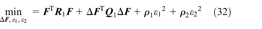
where R₁, Q₁ are weight matrixes; ${\rho }_1$ , ${\rho }_2$ is weight factor;

$$\mathrm{\Delta }\mathit{F}=[\mathrm{\Delta }{F_x}_1,\mathrm{\Delta }{F_x}_2,\mathrm{\Delta }{F_x}_3,\mathrm{\Delta }{F_x}_4{]}^T;F={[F_{x1},F_{x2},F_{x3},F_{x4}]}^T.$$

The first item is used to penalize the system control amount, reflecting the requirement for the maximum value of the control variable; the second item is to penalize the control increment, reflecting the requirement for the steady change of the control quantity; the third and fourth terms introduce relaxation factors to ensure that when the system has no optimal solution within the control horizon, the optimal solution is replaced by the suboptimal solution.

Restrictions are set as formula (33):

$$s.t\{\begin{array}{c}{F}_{\mathrm{xi}\min }\le F_{\mathrm{xi}}\le F_{\mathrm{xi}\max }i=1,2,3,4\hfill \\ \multicolumn{1}{c}{\mathrm{\Delta }{F}_{\mathrm{xi}\min }\le \mathrm{\Delta }{F}_{\mathrm{xi}}\le \mathrm{\Delta }{F}_{\mathrm{xi}\max }i=1,2,3,4}\\ \multicolumn{1}{c}{\mathrm{\Delta }{F}_{\mathrm{xi}}=F_{\mathrm{xi}}-F_{\mathrm{xit}-1}i=1,2,3,4}\\ \multicolumn{1}{c}{0\le {\epsilon }_i\le {\epsilon }_{i\max }i=1,2}\end{array}$$

(33)

where ${F_{\mathrm{xi}}}_{\min }$ and ${F_{\mathrm{xi}}}_{max}$ are the lower limit and upper limit of the control variable respectively; $\mathrm{\Delta }{F_{\mathrm{xi}}}_{\min }$ and $\mathrm{\Delta }{F_{\mathrm{xi}}}_{max}$ are the lower limit and upper limit of the control increment respectively; ${\epsilon }_{imax}$ is the upper limit of the relaxation factor; ${F_{\mathrm{xit}-}}_1$ is the control variable of the previous cycle.

Optimal problem equation (32) is a quadratic programming problem. When the constraints (31) and (33) are satisfied, the optimal control variable $\mathrm{\Delta }F$ is solved to minimize the objective function (32). Transform the quadratic programming problem into a standard form:

$$\underset{\mathit{X}}{min}={\mathit{X}}^{\mathrm{T}}\mathit{HX}+{\mathit{C}}^{\mathrm{T}}\mathit{X}$$

(34)

where

$$\begin{array}{c}\mathit{X}=[\mathrm{\Delta }{\mathit{F}}^{\mathrm{T}},{\epsilon }_1,{\epsilon }_2{]}^{\mathrm{T}}\hfill \\ \mathit{H}=[{\mathit{R}}_1+{\mathit{Q}}_1,0_{4\times 2};0_{2\times 4},{\rho }_1,{\rho }_2]\hfill \\ \mathit{X}=[\mathrm{\Delta }{\mathit{F}}^{\mathrm{T}},{\epsilon }_1,{\epsilon }_2{]}^{\mathrm{T}}\hfill \end{array}$$

Restrictions:

$$s.t\{\begin{array}{c}\mathit{AX}\le \mathit{b}\hfill \\ \multicolumn{1}{c}{\mathit{lb}\le \mathit{X}\le \mathit{ub}}\end{array}$$

(35)

where

$$\mathit{A}=\left[\begin{array}{cccccc}\cos \delta \hfill & \cos \delta \hfill & 1\hfill & 1\hfill & -1\hfill & 0\hfill \\ \multicolumn{1}{c}{-\cos \delta }& -\cos \delta \hfill & -1\hfill & -1\hfill & -1\hfill & 0\hfill \\ \multicolumn{1}{c}{l_a\sin \delta -\frac{c}{2}\cos \delta }& l_a\sin \delta +\frac{c}{2}\cos \delta \hfill & -\frac{c}{2}\hfill & \frac{c}{2}\hfill & 0\hfill & -1\hfill \\ \multicolumn{1}{c}{\frac{c}{2}\cos \delta -l_a\sin \delta }& -l_a\sin \delta -\frac{c}{2}\cos \delta \hfill & \frac{c}{2}\hfill & -\frac{c}{2}\hfill & 0\hfill & -1\hfill \end{array}\right]$$

$$\{\begin{array}{c}l{b}_i=min(F_{\mathrm{xi}\mathrm{m}\mathrm{ax}}-F_{\mathrm{xit}-1},\mathrm{\Delta }{F}_{\mathrm{xi}\max })i=1,2,3,4\hfill \\ \multicolumn{1}{c}{u{b}_i=max(F_{\mathrm{xi}\min }-F_{\mathrm{xit}-1},\mathrm{\Delta }{F}_{\mathrm{xi}\min })i=1,2,3,4}\end{array}$$

$$\mathit{b}=\left[\begin{array}{c}\multicolumn{1}{c}{F_{X\exp }-F_{x1t-1}\cos \delta -F_{x2t-1}\cos \delta -F_{x3t-1}-F_{x4t-1}}\\ \multicolumn{1}{c}{F_{x1t-1}\cos \delta +F_{x2t-1}\cos \delta +F_{x3t-1}+F_{x4t-1}-F_{X\exp }}\\ \multicolumn{1}{c}{M_{Z\exp }-(l_a\sin \delta -\frac{c}{2}\cos \delta )F_{x1t-1}-(l_a\sin \delta +\frac{c}{2}\cos \delta )F_{x2t-1}}\\ \multicolumn{1}{c}{+\frac{c}{2}{F}_{x3t-1}-\frac{c}{2}{F}_{x4t-1}}\\ \multicolumn{1}{c}{(l_a\sin \delta -\frac{c}{2}\cos \delta )F_{x1t-1}+(l_a\sin \delta +\frac{c}{2}\cos \delta )F_{x2t-1}}\\ \multicolumn{1}{c}{-\frac{c}{2}{F}_{x3t-1}+\frac{c}{2}{F}_{x4t-1}-M_{Z\exp }}\end{array}\right]$$

$$\mathit{lb}={[l{b}_1,l{b}_2,l{b}_3,l{b}_4,0,0]}^{\mathrm{T}}$$

$$\mathit{ub}={[u{b}_1,u{b}_2,u{b}_3,u{b}_4,{{\epsilon }_1}_{\max },{{\epsilon }_2}_{\max }]}^{\mathrm{T}}$$

The maximum braking force of the tire is mainly determined by the road adhesion condition and the maximum driving force is also affected by the maximum torque of the in-wheel motor. According to the UniTire model, the maximum and minimum longitudinal force can be obtained by calculating the longitudinal force within the full longitudinal slip ratio range with the vertical load, side slip angle, and wheel center speed as input. Taking into account the error caused by the estimation or parameter changes, the maximum value of the longitudinal force is corrected and adopted as the upper and lower limits of the constraint condition:

$$\rho F_{\mathrm{xi}min}\le F_{x\mathrm{i}}\le min\{\rho F_{\mathrm{xi}max},\frac{T_{max}}{R_e}\},\mathrm{i}=1,2,3,4$$

(36)

where $\rho$ is 0.9; $F_{\mathrm{xi}min}$ is minimum longitudinal force; and $F_{\mathrm{xi}max}$ is maximum longitudinal force.

Simulation and results analysis

The Simulink/Carsim co-simulation platform was built for the simulation verification of the double-line trajectory tracking under different speeds and different road adhesion coefficients. ¹⁷ The CPU of computer is Inter(R) Core(TM) i7-6700 @ 3.40 GHz. In the MPC controller the sample time is 0.02 s. The objective function constructed and the control distributor is solved by the quadratic programming function in MALTAB. The computation time is about six times longer than the simulation time. If the control algorithm is applied to a real vehicle, it is necessary to consider a more optimized solution method, making the algorithm run in a more efficient language environment (such as C language) and using a higher performance processor to ensure the real-time performance of the algorithm. In scenario 1, the adhesion coefficient is 0.8 and the target vehicle speed is 70 km/h.

In scenario 2, the adhesion coefficient is 0.8 and the target vehicle speed is 90 km/h. In scenario 3, the adhesion coefficient is 0.4 and the target vehicle speed is 50 km/h. In scenario 4, the adhesion coefficient is 0.4 and the target vehicle speed is 60 km/h. The effectiveness of the hierarchical controller is verified based on MPC-SMC controller. It is compared with the MPC controller designed in the previous work. ²⁰ In the following, MPC-SMC controller is denoted as controller I and MPC controller is denoted as controller II.

Scenario 1

Figure 5 shows the simulation results and the results obtained in terms of deviation and RMS are listed in Table 2. The deviation and RMS of the lateral position and yaw angle under the controller I are slightly worse than the controller II, but the speed control is far better than the controller II.

Figure 5.

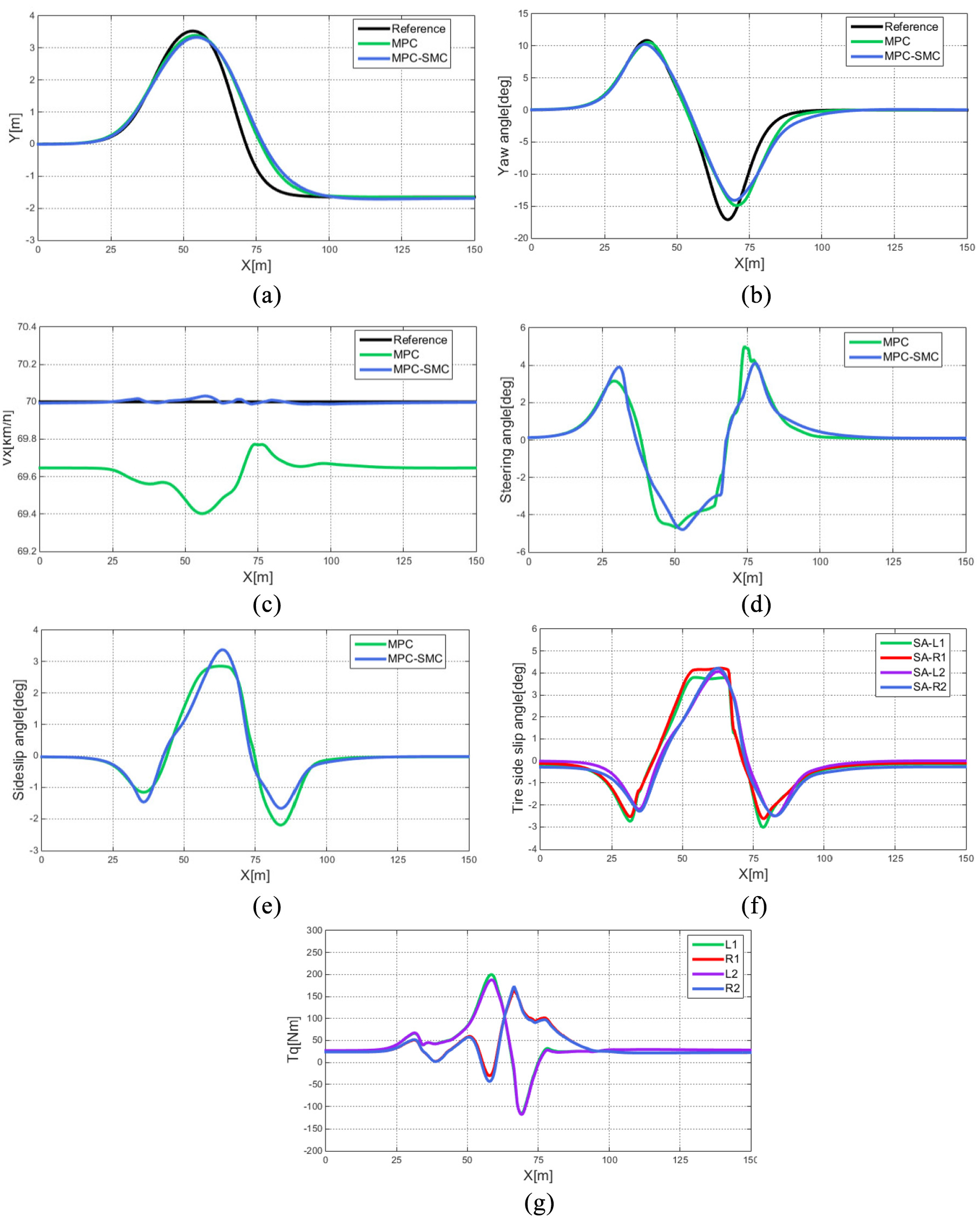
Simulation results under scenario 1: (a) tracking paths, (b) yaw angles, (c) vehicle speeds, (d) steering angles, (e) vehicle mass center sideslip angles, (f) tire side slip angles under controller I, and (g) driving/braking torques under controller I.

Table 2.

Deviation and RMS of results under scenario 1.

	MPC	MPC-SMC
Maximum of lateral deviation	1.09 m	1.24 m
RMS of lateral deviation	0.33 m	0.39 m
Maximum of Yaw angle deviation	4.10°	4.34°
RMS of yaw angle deviation	1.32°	1.48°
Maximum of vehicle speed deviation	0.60 km/h	0.03 km/h
RMS of vehicle speed deviation	0.38 km/h	0.009 km/h

It can be seen from Figure 5(d) that the maximum front wheel angle under controller I is 4.79° while that under controller II is 5.00°. The difference between the two results is small. Figure 5(e) shows the vehicle mass center sideslip angle under controller I and II. The maximum vehicle sideslip angle under controller I is 3.37° while that under controller II is 2.86°. They are both lower than the stability threshold 8.91°. ²⁸ It can be seen from Figure 5(f) that the maximum tire side slip angles of the front left, front right, rear left, and rear right wheels are 3.79°, 4.22°, 4.07°, and 4.21° respectively, which all meet the soft-constraint condition. It can be seen from Figure 5(g) that the maximum driving/braking torques of the front left, front right, rear left, and rear right wheels are 199.93, 165.35, 187.78, and 173.04 N m respectively, which all meet the constraint condition.

Scenario 2

Figure 6 shows the simulation results and the results obtained in terms of deviation and RMS are listed in Table 3. The deviation and RMS of the lateral position and yaw angle under the controller I are slightly better than the controller II and the speed control is far better than the controller II.

Figure 6.

Simulation results under scenario 2: (a) tracking paths, (b) yaw angles, (c) vehicle speeds, (d) steering angles, (e) vehicle mass center sideslip angles, (f) tire side slip angles under controller I, and (g) driving/braking torques under controller I.

Table 3.

Deviation and RMS of results under scenario 2.

	MPC	MPC-SMC
Maximum of lateral deviation	3.13 m	3.00 m
RMS of lateral deviation	1.10 m	1.04 m
Maximum of Yaw angle deviation	10.22°	9.49°
RMS of yaw angle deviation	3.66°	3.53°
Maximum of vehicle speed deviation	0.89 km/h	0.05 km/h
RMS of vehicle speed deviation	0.50 km/h	0.02 km/h

It can be seen from Figure 6(d) that the maximum front wheel angle under controller I is 4.64° while that under controller II is 5.57°. The difference between the two results is small. Figure 6(e) shows the vehicle mass center sideslip angle under controller I and II. The maximum vehicle sideslip angle under controller I is 6.63° while that under controller II is 3.99°. They are both lower than the stability threshold 8.91°. ²⁸ It can be seen from Figure 6(f) that the maximum tire side slip angles are 5.27°, 5.86°, 6.36°, and 6.75° respectively, which all meet the soft-constraint condition. It can be seen from Figure 6(g) that the maximum driving/braking torques are 369.12, 167.87, 354.03, and 183.29 N m respectively, which all meet the constraint condition.

Scenario 3

Figure 7 shows the simulation results and the results obtained in terms of deviation and RMS are listed in Table 4. The deviation and RMS of the lateral position and yaw angle under the controller I are not much different from the controller II and the speed control is far better than the controller II. It can be seen from Figure 7(d) that the maximum front wheel angle under controller I is 4.94° while that under controller II is 4.04°. The front wheel angle under controller I is a little larger than that under controller II. Figure 7(e) shows the vehicle mass center sideslip angle under controller I and II. The maximum vehicle sideslip angle under controller I is 0.86° while that under controller II is 1.60°. They are both lower than the stability threshold 4.48°. ²⁸ It can be seen from Figure 7(f) that the maximum tire side slip angles are 3.19°, 3.29°, 2.23°, and 2.05° respectively, which all meet the soft-constraint condition. It can be seen from Figure 7(g) that the maximum driving/braking torques are 49.56, 37.31, 48.83, and 36.76 N m respectively, which all meet the constraint condition.

Figure 7.

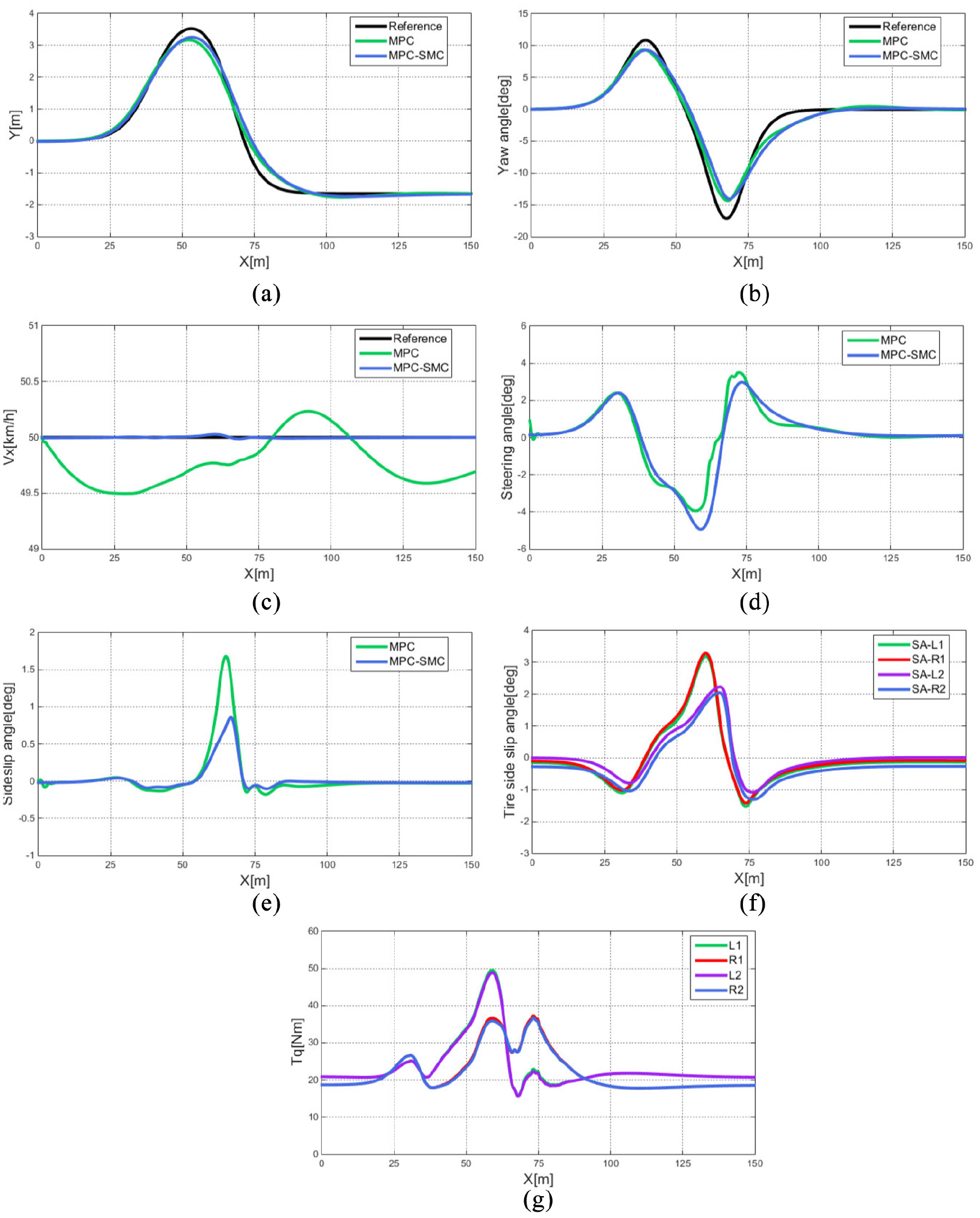
Simulation results under scenario 3: (a) tracking paths, (b) yaw angles, (c) vehicle speeds, (d) steering angles, (e) vehicle mass center sideslip angles, (f) tire side slip angles under controller I, and (g) driving/braking torques under controller ã.

Table 4.

Deviation and RMS of results under scenario 3.

	MPC	MPC-SMC
Maximum of lateral deviation	0.44 m	0.60 m
RMS of lateral deviation	0.19 m	0.20 m
Maximum of Yaw angle deviation	2.94°	4.14°
RMS of yaw angle deviation	1.09°	1.40°
Maximum of vehicle speed deviation	0.50 km/h	0.03 km/h
RMS of vehicle speed deviation	0.32 km/h	0.007 km/h

Scenario 4

Figure 8 shows the simulation results and the results obtained in terms of deviation and RMS are listed in Table 5. The deviation and RMS of the lateral position and yaw angle under the controller I are a little lower than the controller II but the speed control is far better than the controller II.

Figure 8.

Simulation results under scenario 4: (a) tracking paths, (b) yaw angles, (c) vehicle speeds, (d) front wheel steering angles, (e) vehicle mass center sideslip angles, (f) tire side slip angles under controller I, and (g) driving/braking torques under controller I.

Table 5.

Deviation and RMS of results under scenario 4.

	MPC	MPC-SMC
Maximum of lateral deviation	1.05 m	1.55 m
RMS of lateral deviation	0.36 m	0.52 m
Maximum of Yaw angle deviation	5.33°	7.37°
RMS of yaw angle deviation	2.04°	2.45°
Maximum of vehicle speed deviation	0.72 km/h	0.03 km/h
RMS of vehicle speed deviation	0.47 km/h	0.009 km/h

It can be seen from Figure 8(d) that the maximum front wheel angle under controller I is 4.63° while that under controller II is 3.08°. Figure 8(e) shows the vehicle mass center sideslip angle under controller I and II. The maximum vehicle sideslip angle under controller I is 2.03° while that under controller II is 2.60°. They are both lower than the stability threshold 4.48°. ²⁹ It can be seen from Figure 8(f) that the maximum tire side slip angles are 3.78°, 3.90°, 3.04°, and 2.88° respectively, which all meet the soft-constraint condition. It can be seen from Figure 8(g) that the maximum driving/braking torques are 85.75, 58.89, 81.95, and 59.73 N m respectively, which all meet the constraint condition.

Conclusion

A UniTire model under complex wheel motion inputs is adopted and the model parameters are solved by fitting the multi conditions test data in this paper. On the one hand, it improves the expression accuracy of the tire model, on the other hand, it facilitates the practical application of the algorithm based on the UniTire model structure features. With the characteristics of physical model background, unified normalized expression of slip ratio and forces, and the inserted friction coefficient, UniTire which model parameters fitted from test condition is convenient for application under different working conditions with high accuracy. For four-wheel independent drive intelligent vehicle, the longitudinal and lateral motion control of the vehicle are decoupled. Based on MPC and SMC, a hierarchical controller is designed to track the reference trajectory and expected vehicle speed simultaneously. A new approach law is adopted in the SMC of vehicle speed which can further weaken the chattering of the system while ensuring fast convergence to the sliding mode surface. The quadratic planning method is used in the control distributor to distribute the total yaw moment calculated by the MPC and the total longitudinal force calculated by the SMC, that takes into account the road adhesion conditions and the constraints of the actuator. The feasibility and accuracy of the designed controller was verified through CarSim/Simulink co-simulation. The MPC-SMC controller is significantly better than the MPC controller in speed control. The difference in the tracking accuracy of the lateral position and yaw angle is small.