Sage Journals: Discover world-class research

Abstract

Knowledge of frame loads at the limits of the intended driving conditions is important during the design process of a vehicle structure. Yet, retrieving these loads is not trivial as the load path between the road and the frame mounting point is complex. Fortunately, recent studies have shown that multibody dynamic (MBD) simulations could be a powerful tool to estimate these loads. Two main categories of MBD simulations exist. Firstly, full analytical simulations, which have received great attention in the literature, are run in a virtual environment using a tire model and a virtual road. Secondly, hybrid simulations, also named semi analytical, uses experimental data from Wheel Force Transducers and Inertial Measurement Units to replace the road and tire models. It is still unclear how trustworthy semi analytical simulations are for frame load evaluation. Both methods were tested for three loads cases. It was found that semi analytical simulations were slightly better in predicting vehicle dynamic and frame loads than the full analytical simulations for frequencies under the MF-Tyre model valid frequency range (8 Hz) with accuracy levels over 90%. For faster dynamic maneuvers, the prediction accuracy was lower, in the 50%–80% range, with semi analytical simulations showing better results.

Keywords

Frame loads vehicle dynamics multibody dynamics MBD hybrid simulation

Introduction

Each time a new vehicle is considered for development, the mechanical structure design is often revisited with the purpose of reducing its weight, while improving several other related aspects, including style, handling behavior, or manufacturability. The redesign process greatly benefits from a thorough knowledge of the vehicle operating loads. Reliable and valid estimation of these loads is not a straightforward task. Indeed, the load path between ground inputs to the mounting points on the frame is influenced by numerous vehicle components such as tires, bushings, suspensions, or suspension arms.

Various methods have been suggested in the literature to retrieve frame loads during dynamic maneuvers. For instance, load sensors at the mounting points can be used to retrieve loads at the suspensions and heavy parts mounting points. However, the vehicle dynamics can be modified by those sensors, thus impacting load data validity.¹ Also, some mounting points on a structure may be inaccessible by load sensors due to space constraints. As a mitigation strategy, researchers have suggested using load correlation from strain gauges installed on flexible parts.² This method is yet limited to the extent of the load correlation performed whether it was considered uniaxial or multiaxial. Although some load directions are predominant (i.e. vertical axis while driving on a bumpy road), loads transmitted to the frame are multiaxial in nature during normal driving conditions.³ Frame and suspension arms flexibility have also an impact on the transmitted loads to the frame. In fact, Chen and Wang⁴ showed that flexible elements in a vehicle structure also store potential energy that impacts vehicle behavior.

Lastly, Multi-Body Dynamic (MBD) models of vehicles were proposed to retrieve input loads. Two main methods are currently used in MBD simulations. The first one is based on a virtual road and a prior characterization of tires.^4–7 This method, also named full analytical by some authors, uses a vehicle model that is kinematically guided to navigate in a virtual environment. The method is often used, and it has been tested in the past. Alternatively, hybrid simulation methods also exist where the tire model and the virtual road are not needed and are replaced by experimental data. These methods, also named semi analytical by some authors, are less frequent in the literature and are less popular to retrieve frame loads in a dynamically moving vehicle. Usually, wheel force transducers (WFTs) that record forces and moments exerted on the wheel hub are used to acquire field data necessary for semi analytical simulations, in conjunction with kinematic data collected using inertial measurement units (IMU).^2,8–10

Numerous semi analytical simulation methods have been described in the literature. Some are solely based on WFTs data. For instance, the Grounded Chassis method (GC)^11,12 uses a vehicle MBD model grounded at a fixed joint while WFTs recorded efforts are transmitted to the vehicle hubs. In the Controlled Chassis around Origin method (CCO),¹² the MBD model is free to move about a fixed point through a spring-damper connection, while WFTs efforts are transmitted to the hubs. Other methods use both WFTs and IMU data. The Moved Chassis to a Recorded Position method (MCRP)^12,13 constrains the vehicle body to follow a recorded time varying trajectory while exerting the WFTs efforts to the wheel hubs. Finally, in the Controlled Chassis around a Recorded Position method (CCRP),^12,13 the MBD model is free to move about a recorded time varying trajectory through a spring-damper connection, while WTFs efforts are transmitted to the vehicle.

Joubert et al.¹² previously showed that the CCRP method is the most accurate semi analytical method by simultaneously taking into account load transmission, vehicle orientation, and inertial effects with an acceptable level of non-causal corrective loads by the controller. Semi analytical simulations using the CCRP method connect the vehicle center of gravity (CoG) to a time-varying point trajectory through spring-damper connections along the six degrees of freedom (DoF). If the vehicle motion resulting from the WFTs efforts exerted at the wheel hubs is different from the dynamics registered by the IMU, corrective efforts are applied at the frame CoG. These corrective forces can impact frame load evaluation if their amplitudes are significant.¹² Although the study conducted by Jouvert et al. highlighted the importance of boundary conditions on semi analytical simulation results, simulations were performed using virtual input data previously computed from a full analytical MBD vehicle model simulation. Hence, the effectiveness of the method with experimental data is yet to be proven.

Advantages and disadvantages of using semi analytical simulations over full analytical ones were well covered by Joubert et al.¹² In a full analytical simulation, a road profile and a tire model are needed, along with the tire model commercial license. Obtaining road profiles and tire models are expensive and time-consuming tasks. Also, controlling the vehicle path along a given track may be difficult as inaccuracies in the steering orientation can lead to large position drifts during long simulations. These problems are prevented with semi analytical simulations since they are independent of road characterization, and they do not rely on tire models due to availability of WFTs data. Semi analytical simulations also cover a larger frequency spectrum since WFTs bandwidth is currently in the range of 1000 Hz, while tire models are valid in a range below 250 Hz. Higher frequency content may be needed for durability or NVH analysis. Yet, semi analytical simulations are limited to the specific test runs performed and a vehicle prototype must be built and instrumented to gather the input data for the simulations. In addition, instrumentation can add significant weight to a vehicle, particularly in lightweight vehicles such as recreational vehicles. Thus, assumptions must be made while using the experimental data in semi analytical simulations such that the efforts transmitted to the frame are not over-evaluated compared to a standard non-instrumented production vehicle.

The scope of this study was to evaluate the accuracy of the semi analytical CCRP method, using experimentally acquired data signals as inputs. In order to do so, semi analytical simulations were compared with their equivalent full analytical simulations and experimental data obtained for different vehicles maneuvers. Prediction of frame loads was performed in a three-wheeled vehicle using an MBD model with a rigid frame and flexible suspension arms.

Methodology

Vehicle models and general testing protocol

The full analytical simulation developed used an MF-Tyre model^14,15 and an OpenCRG road (OpenCRG, Bad Aibling, Germany) while the semi analytical simulations used the CCRP method with IMU and WFTs data. Accuracy of both methods was evaluated by recording suspension displacements and strain at specific points in the a-arm and swing arm of the vehicle. Three different maneuvers were used to evaluate the accuracy of full and semi analytical MBD methods. These maneuvers loaded the vehicle laterally and vertically with moderate to high intensity.

Both simulation methods are based on the same vehicle MBD model, developed on MotionView (Altair Engineering, Troy, MI, USA) with mass and inertia calibrated with measurements from a reference test vehicle.

Instrumented vehicle

The test vehicle was instrumented with numerous sensors to record the vehicle dynamics and road inputs. Linear potentiometers were used on the front suspension and a rotational potentiometer was used on the rear suspension to measure suspension travels. Directional strain gauges and a rosette were used on the suspension arms to record local strains. Wheel Force Transducers (WFT) (Michigan Scientific Corporation, Milford, USA) were used on each wheel to record forces and torques at the hubs. An Inertial Measurement Unit (IMU) (OXTS, Middleton Stoney, United Kingdom) was used to record the vehicle kinematics. Finally, the steering angle was recorded using the vehicle CAN Bus. The instrumentation is listed in Table 1.

Table 1.

Vehicle instrumentation.

Instrumentation	Location	Readings	Sampling rate (Hz)
2 × linear potentiometers	On each front suspension	Travel of the front suspensions	2000
1 × rotational potentiometer	On the rear suspension	Travel of the rear suspension	2000
1 × IMU	On the front of the vehicle mounted on a custom rigid bracket	Linear and angular position, speed and acceleration of the vehicle	200
3 × Wheel force transducers (WTF)	On each wheel	Forces and torques at the wheel hubs Wheel angular velocity	1000
Vehicle CAN bus	From the vehicle on-board computer	Steering angular position	100
1 × directional strain gauge (J1)	On the vehicle left lower a-arm (Figure 3)	Directional strain	2000
1 × 45° rosette (JSA1)	On the left side of the swing arm (Figure 3)	Principal and Von Mises strains	2000

Strain gauge and rosette placements were based on a finite element analysis of the static load cases of the vehicle to determine the areas where the strain variation amplitude was high enough to provide good readings for the three test maneuvers. Positions of gauge J1 and JSA1 are shown in Figure 1.

Figure 1.

Strain gauges positioning.

Maneuvers

Three maneuvers were tested: a double lane change, a hard braking, and a speed bump. The double lane change laterally loaded the vehicle with moderate amplitude. Braking longitudinally loaded the vehicle with high amplitude. Finally, the speed bump vertically loaded the vehicle with high amplitude.

Double lane change (DLC)

This maneuver consisted in accelerating the vehicle in the right lane up to a desired speed. Then, at the “throttle release” point (12 m before the start of the lane change), the pilot released the throttle and disengaged the clutch before proceeding to the lane change (Figure 2). The vehicle approach speed was iterated in order to find the maximum speed that would not trigger the vehicle stability system. An initial speed of 38 km/h was thus selected for the test. This maneuver induced moderate lateral stress to the vehicle, generating roll and yaw motion. This test is inspired by the International Standard ISO 3888-2 norm.¹⁶

Figure 2.

Double lane change test dimensions.

Braking

The pilot was instructed to reach a constant speed of 75 km/h. Then, the pilot braked as hard as he could in a straight line without locking the wheels until he brought the vehicle to a stop. This maneuver induces high longitudinal loads on the vehicle.

Speed bump

The pilot was instructed to reach a constant speed of 30 km/h. Then, approximately 1.85 m before the speed bump (Figure 3), the pilot disengaged the clutch, inducing high vertical loads on the vehicle.

Figure 3.

Speed bump dimensions.

MBD vehicle model

The MBD model developed is a three-wheeled recreational vehicle (Figure 4). The frame is a steel tube welded construction. The front suspension system is a double a-arm type, the rear suspension system is a swing arm type and the steering system is a single pitman arm type with a handlebar. The engine is fixed on the frame with three rubber mounts to limit vibration transmission to the frame. The mounts, the a-arm, and swing arm pivots were modeled as linear bushings (with constant stiffness and damping coefficient values in each DoF). For each a-arm and swing arm, a Craig-Bampton modal reduction^4,7,17 was performed on OptiStruct (Altair Engineering, Troy, MI, USA) to create flexible elements for dynamic simulations. Modes up to 4000 Hz were considered for the model. The frame was modeled as a rigid body. The software MotionView (Altair Engineering, Troy, MI, USA) was used to build the MBD model and MotionSolve (Altair Engineering, Troy, MI, USA) was used to performed the full and semi analytical simulations using a fixed 0.0001 s time step.

Figure 4.

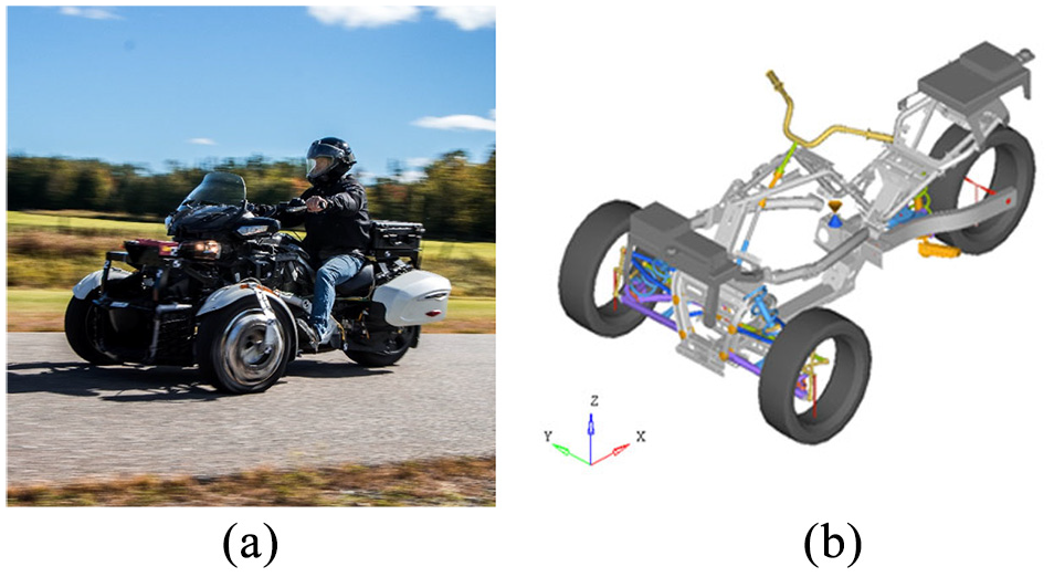
Instrumented test vehicle (a) and vehicle MBD model (b).

The MBD model was constructed based on the CAD model geometry of the vehicle. The points of contact between the different vehicle bodies were identified and the joint type and orientation of the joints were assigned. A mass and an inertia values were determined for each body based on experimental measurements and CAD values. The suspension submodels were then integrated into the overall model. The suspension submodel was constructed based on experimental curves for both the springs and dampers. The bump and rebound stops locations as well as their experimentally characterized behavior were added to this submodel. Furthermore, the experimental characteristics of the different bushings used on the vehicle were introduced into the model. Finally, the flexible a-arms and swing arm were connected with their respective joint into the model.

The total mass of the vehicle, including the frame, the powertrain and the test instrumentation was 490 kg. An 80 kg pilot was also modeled as a rigid body fixed to the frame.

Weight and Inertia calibration of the MBD model

The vehicle was placed on digital scales, one under each of the three wheels. Scales under the front wheels were installed on rollers to compensate for the vehicle track width change caused by the displacement of the front suspension under load. Two conditions were analyzed:

Condition 1: Flat ground.

Condition 2: Horizontal vehicle being pitched backward by lifting the front wheels by 30 cm.

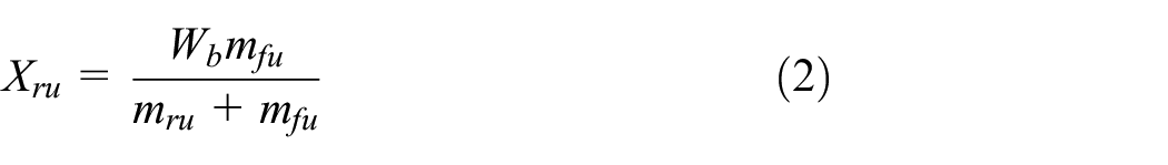
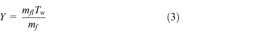
Mass measurements were recorded for both conditions for each scale. The X, Y, Z positions of the center of gravity (CoG) were determined using the equations below:

X_{r} = \frac{W_{b} m_{f}}{m_{r} + m_{f}}

(1)

X_{ru} = \frac{W_{b} m_{fu}}{m_{ru} + m_{fu}}

(2)

Y = \frac{m_{fl} T_{w}}{m_{f}}

(3)

Z = \frac{X_{r} \cos (a) - X_{ru}}{\sin (a)} + Z_{wr}

(4)

where $X_{r}$ is the CoG position measured from the center of the rear wheel (Figure 5), $W_{b}$ is the wheelbase length, $m_{f}$ is the total mass readings on the front scales (both left and right), $m_{r}$ is the mass reading on the rear scale, $Y$ is the CoG position measured from the right front wheel, $T_{w}$ is the track width, $a$ is the pitch angle variation achieved from raising the front wheel in Condition 2, $Z$ is the CoG position measured from the ground and $Z_{wr}$ is the radius of the rear wheel. The subscript “u” means that this variable comes from the scale measurements when the front of the vehicle is raised (Condition 2) and “ l ” is the value measured on the left scale. Equation (4) is based on the assumptions that the suspension compression and wheelbase variations are constant in the horizontal (Condition 1) and pitched (Condition 2) conditions.

Figure 5.

CoG position variables.

Vehicle inertia characteristics were computed based on CAD inertia values of the different 3D modeled parts and inertia measurements from a similar three-wheeled vehicle (albeit 16% lighter) that was characterized in the past ( $I_{light - vehicle}$ ). As an approximation, it was assumed that the inertia values of the heavier instrumented test vehicle would scale up proportionally with the mass increase. Since most of the small parts are not physically represented in the MBD model (wiring, fuel, bodywork, sensors, bolts, electronics, etc.), their impact on the total inertia was considered by adding a dummy body rigidly fixed on the frame at the CoG of the vehicle with the appropriate inertia values so that the MBD model has the same inertia as the test vehicle. To determine the dummy body inertia values ( $I_{CoG}$ ), equation (5) was used where the inertia relative to the CoG of the vehicle of each modeled part ( $I_{i} |_{CoG}$ ) is subtracted from the estimated total inertia of the test vehicle. $I_{i} |_{CoG}$ is determined using the parallel axis theorem (equation (6)).

I_{CoG} = I_{light - vehicle} \times \frac{M_{test - vehicle}}{M_{light - vehicle}} - \sum_{i = 1}^{nbr parts} I_{i} |_{CoG}

(5)

I_{i} |_{CoG} = {\bar{I}}_{i} + m_{i} d_{i}^{2}

(6)

where ${\bar{I}}_{i}$ is the inertia of a part about its own center of mass, $m_{i}$ is the mass of the different parts, $d_{i}$ is the distance to the vehicle CoG of these part’s CoGs, $M_{test - vehicle}$ is the mass of the instrumented vehicle and $M_{light - vehicle}$ is the mass of the similar lighter three-wheeled vehicle.

In the case that vehicle inertia values are unknown and comparable vehicle data is not available, other authors have used dual extended Kalman filter (DEFK)¹⁸ and dual unscented Kalman filter (DUFK)¹⁹ that simultaneously estimate the vehicle states and inertial parameters. These Kalman filter-based estimations use input data from sensors such as steering angle, wheel speed, and wheel torque. Jin et al.¹⁹ and Antonov et al.²⁰ have shown that UFK approaches have better accuracy and robustness at the cost of a slightly higher computational time.

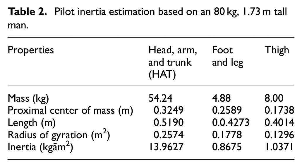
As for the 80 kg, 1.73 m tall pilot, the inertia properties were based on anthropometric data from Table 4.1 of Winter²¹ and Table 2 of Ramachandran et al.²² The pilot body is subdivided in five segments and their corresponding masses and inertiae were computed using estimations in Table 2.

Table 2.

Pilot inertia estimation based on an 80 kg, 1.73 m tall man.

Properties	Head, arm, and trunk (HAT)	Foot and leg	Thigh
Mass (kg)	54.24	4.88	8.00
Proximal center of mass (m)	0.3249	0.2589	0.1738
Length (m)	0.5190	0.0.4273	0.4014
Radius of gyration (m²)	0.2574	0.1778	0.1296
Inertia (kgãm²)	13.9627	0.8675	1.0371

Full analytical simulation

For the full analytical simulations, the MBD model described in Section 3.4 is used with an MF-Tyre model.¹⁴ This model is known as an industry standard for vehicle handling simulations. Both front and rear tires were characterized regarding cornering and vertical stiffness and damping, etc. The tire model validity is limited when simulating uneven roads, frequency inputs over 8 Hz and large tire deformations. Road surfaces are modeled using the OpenCRG protocol (OpenCRG, Bad Aibling, Germany) which is commonly used for tire/driving/vibration simulations.

For higher vehicle speeds (over 15 km/h), aerodynamic drag resistance (F_x) is non-negligible. It is modeled using equation (7) and it is exerted at the center of mass of the vehicle as a first approximation:

F_{x} = \frac{1}{2} ρ C_{x} A V^{2}

(7)

where ρ is the air density (ρ = 1.225 kg/m³), C_xA is the product of the frontal area and the drag coefficient, and V is the longitudinal speed relative to airspeed.

For each maneuver, the vehicle is accelerated to the desired initial speed by applying a force on the frame at the vehicle CoG. For the braking maneuver, the wheels angular velocities are controlled using experimental data curves by applying a torque between the spindle and the knuckle. This allows the braking torques to be simulated while decelerating. Similarly, the steering angular position is also controlled at the revolute joint, where the handlebar connects with the steering column, using experimental data for the DLC maneuver.

Semi analytical (hybrid) simulation

The hybrid method used in this study is based on the “controlled around a recorded position – CCRP” method described by Joubert et al.¹² The MBD model described in Section 3.4 is used but instead of adding a virtual road and a tire model as performed in the full analytical simulation, forces and moments equivalent to WFTs load signals are applied at the wheel hubs as inputs to the semi analytical model. The wheel hub angular velocities are also specified at the hub’s revolute joints as prescribed motions. By controlling wheel angular velocities, the gyroscopic torques are more accurately transmitted to the frame.

In order to prevent unacceptable spatial drift of the vehicle over time, the vehicle frame kinematics must be specified along 6 DoFs. This is achieved by connecting the frame at its center of gravity with a compliant joint to a massless dummy body which kinematics are prescribed over time. Along the three rotational DoFs of the dummy body, orientation data from the IMU is used. For the three translations of the dummy body, estimates of CoG velocity are computed from the IMU data, and they are prescribed along the three translational DoFs, instead of positioning data which are less reliable.

The role of the compliant joint is to allow the vehicle frame to react to the WFTs inputs while correcting the positioning errors over time and transmitting minimal corrective efforts to the frame. The compliant joint is tuned to be critically damped (ζ = 1) with a minimal stiffness while ensuring adequate translational velocities and angular positioning during high dynamic maneuvers. For the simulated maneuvers that were investigated, a natural frequency of 5 rad/s (0.8 Hz) was found to be satisfactory for the compliant joint mechanical impedance. The equations used to tune the compliant joint are the following:

ω_{n} = \sqrt{\frac{k}{m}} or ω_{n} = \sqrt{\frac{k_{θ}}{I}}

(8)

ξ = \frac{c}{2 m ω_{n}} or ξ = \frac{c_{θ}}{2 I ω_{n}}

(9)

where $ω_{n}$ is the natural frequency along a given DoF, k is the connecting joint stiffness along that DoF, m is the vehicle mass, c is the damping coefficient along that DoF, I is the inertia of the vehicle about that DoF and the subscript θ is used to distinguish the rotational cases from the translational ones.

The 6 DoFs controller that emulated the compliant joint is sensitive to the resolution and to the noise in the linear velocities and angular positions of the vehicle. In fact, the solver exerts forces and moments to the dummy body to control its position. To determine these efforts, the solver derives these trajectory kinematics data to determine a corresponding acceleration. If the resolution is low or noise is substantial, large accelerations can occur, inducing considerable corrective efforts on the frame. Therefore, translational velocities, angular positions, and wheel speed data were processed using a low-pass ideal filter with a 50 Hz cut-off frequency (Table 3).

Table 3.

Experimental input data for the semi analytical simulations.

Signals (sensors)	Bandwidth (Hz)	Filtering
Linear velocity Vx, Vy, Vz (IMU)	200	Ideal low-pass (cut-off at 50 Hz)
Angular position Rx, Ry, Rz (IMU)	200	Ideal low-pass (cut-off at 50 Hz)
Hubs’ efforts Fx, Fy, Fz, Mx, My, Mz (WFTs data)	1000	No filtering
Wheel angular speed (WFTs)	1000	Ideal low-pass (cut-off at 50 Hz)
Steering angle (CAN Bus)	100	No filtering

The steering angle motion is prescribed at the revolute joint where the handlebar connects with the steering column. This modifies front wheel orientation, thereby creating gyroscopic moments that are transmitted to the frame.

Figure 6 summarizes the test data that were acquired for elaborating the semi analytical MBD simulations. Initial translational and rotational velocities of the different bodies were implemented as initial conditions to the model.

Figure 6.

Test data used in the semi analytical MBD simulations.

Results

Three maneuvers were investigated. For each maneuver, the WFTs data are presented to provide a general idea of the input forces and moments exerted on the wheel hubs. The x-axis data are illustrated in green, the y-axis data are illustrated in blue and the z-axis data are illustrated in black. The results obtained by the full and semi analytical simulations are compared to the experimental measurements and are presented at the end of the WFTs data plots. For each maneuver, time domain measurements of the front left and rear suspension travel, the upper left a-arm, and the swing arm strain gauge data are presented. Right suspension travel is not presented as the right potentiometer broke during the test campaign. Each graph includes the full analytical results in blue, the semi analytical results in black and experimental measurements in green. Finally, a table summarizes the results by giving the standard deviation ( $σ$ ) and the coefficient of determination (R²) of the suspension travels and strains time signals. Also, in Section 4.4, the corrective forces and moments applied on the vehicle’s frame by the spring-damper controller during the semi analytical simulations are presented to assess the impact of the controller on the vehicle kinematics.

Even though the goal of this study is to predict the input frame loads and that the MBD model developed can easily simulate these loads, no experimental force data was recorded at the frame interface as mounting points are not readily accessible. It is assumed in this study that if the suspension displacements and the strains in the flexible parts of the vehicle correlate with the experimental data, then the loads simulated will correlate in a similar manner.

Double lane change (DLC)

For the DLC simulation, the recorded steering position is used to specify front wheels orientation in the MBD model. This input allows the vehicle to steer in the full analytical simulations while it simply changes front wheels orientation in the semi analytical simulations, allowing simulation of gyroscopic loads. In the full analytical simulation, the vehicle is speed-controlled at the beginning of the simulation until it reaches the vehicle experimental speed.

Figures 7 to 9 show the WFT forces and moments amplitudes during the DLC test. Forces in the vertical direction (z-axis) peaked at around 1000 N, while moments in the X direction reached close to 300 Nm.

Figure 7.

Experimental hub forces and moments at the front left wheel for the DLC test (sampling rate of 1000 Hz).

Figure 8.

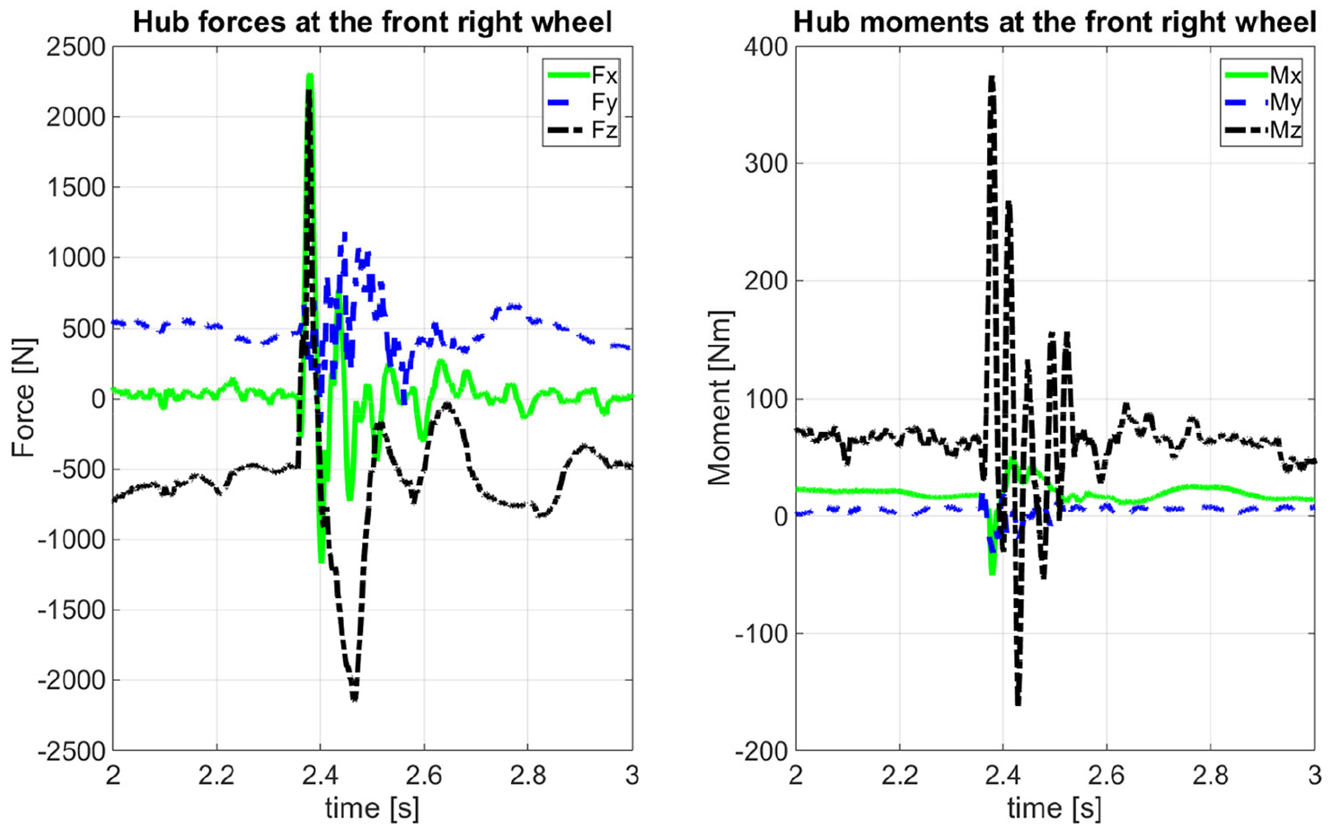
Experimental hub forces and moments at the front right wheel for the DLC test (sampling rate of 1000 Hz).

Figure 9.

Experimental hub forces and moments at the rear wheel for the DLC test (sampling rate of 1000 Hz).

Figures 10 and 11 show the suspension positions and the strain obtained from the a-arm gauge (JAA) and the swing arm gauge (JSA). The simulated strain values were corrected to fit the zero output of the strain gauges which is set with the vehicle resting on the ground without a pilot.

Figure 10.

Suspension position amplitudes for the left shock (left) and the rear shock (right) in the DLC test.

Figure 11.

Strain amplitudes in the upper left a-arm (left) and the swing arm (right) for the DLC test.

Simulation results for both full and semi analytical simulations show comparable behavior with experimental data (Table 4). In fact, standard deviations are small and the coefficient of determination is always above 95% for every metric. Semi analytical simulation shows slightly more accurate results.

Table 4.

Standard deviation and coefficient of determination for the DLC test calculated between 1 and 7 s.

Variables	Standard deviation (σ)	Coefficient of determination (R²)²³
Left shock position (Full)	1.13 mm	0.97
Left shock position (Semi)	0.94 mm	0.99
JSA strain (Full)	2.35 µstrain	0.98
JSA strain (Semi)	2.62 µstrain	0.97
JAA strain (Full)	13.35 µstrain	0.97
JAA strain (Semi)	7.92 µstrain	0.99

Braking

For the braking maneuver, the vehicle speed is controlled while accelerating the vehicle from a still position to a constant speed of 75 km/h. Steering input is not used in the simulations as the steering angle remains constant at 0° during the maneuver. When the vehicle is decelerating in the full analytical simulation, the wheel speed is controlled by applying a torque between the spindle and the knuckle thus simulating the braking torque. On the figures below, only the decelerating part between 75 m/ph and 35 km/h is shown.

Figures 12 to 14 show the WFT forces and moments amplitudes during the braking maneuver. Forces in the longitudinal direction (x-axis) peaked at around 2000 N at the front wheels. Moments in the y-axis at the front wheels were also significant, peaking over 500 Nm. Braking simulation data were compared to experimental data by analyzing the position of the suspensions and the strain amplitude in the suspension arms (Figures 15 and 16). The simulated strain values were corrected to fit the zero output of the strain gauges which were set with the vehicle resting on the ground without a pilot.

Figure 12.

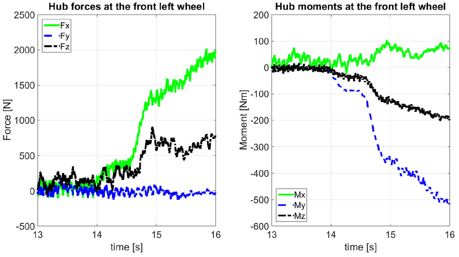
Experimental hub forces and moments at the front left wheel for the braking test (sampling rate of 1000 Hz).

Figure 13.

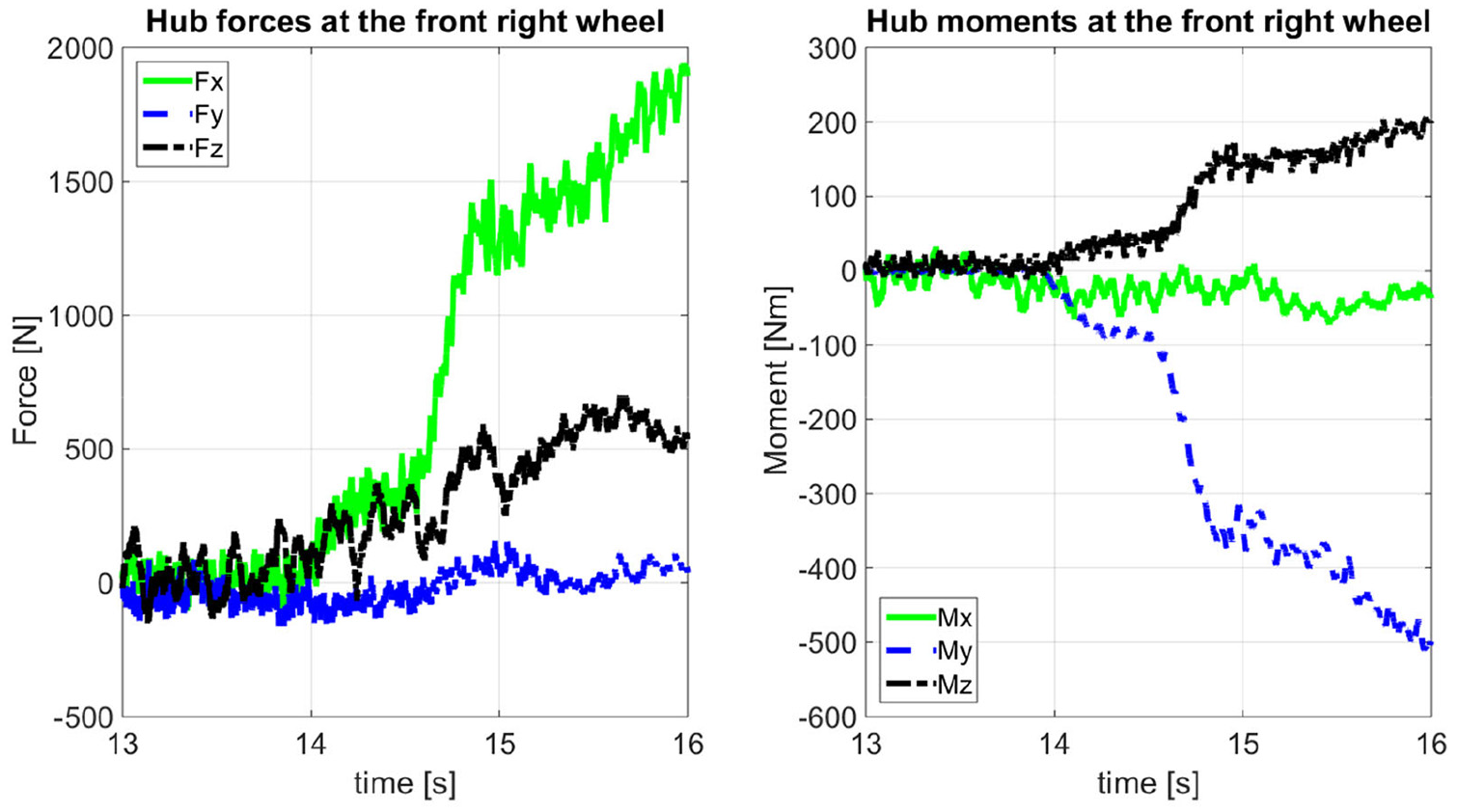
Experimental hub forces and moments at the front right wheel for the braking test (sampling rate of 1000 Hz).

Figure 14.

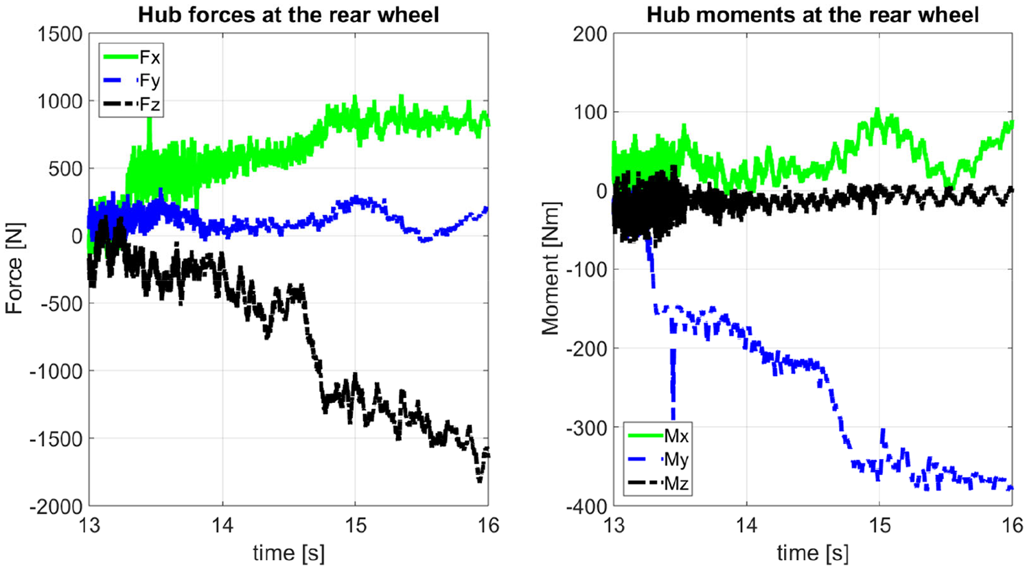
Experimental hub forces and moments at the rear wheel for the braking test (sampling rate of 1000 Hz).

Figure 15.

Suspension positions amplitudes for the left shock (left) and the rear shock (right) for the braking test.

Figure 16.

Strain amplitudes in the upper left a-arm (left) and the swing arm (right) for the braking test.

In the above figures, the pilot disengages the clutch at around 13.2 s and start braking at around 14 s. At 14 s, the vehicle is at 75 km/h while 2 s later it is at 35 km/h.

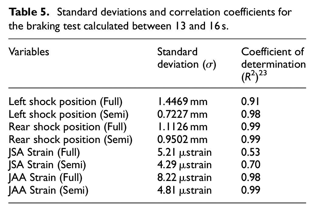
Simulation results for both full and semi analytical simulations show comparable behavior with experimental data albeit slightly better for the semi analytical (Table 5). In fact, standard deviations are small and the coefficient of determination is always above 90% for every metric except for the strain in the swing arm. As seen in Figure 16 (right), the strain variation in the swing arm is low while the high frequency input from the tires on the road and the engine is notable. As seen on the semi analytical curve, some of this high frequency noise was simulated since the WFT data had enough bandwidth and resolution to measure this input.

Table 5.

Standard deviations and correlation coefficients for the braking test calculated between 13 and 16 s.

Variables	Standard deviation (σ)	Coefficient of determination (R²)²³
Left shock position (Full)	1.4469 mm	0.91
Left shock position (Semi)	0.7227 mm	0.98
Rear shock position (Full)	1.1126 mm	0.99
Rear shock position (Semi)	0.9502 mm	0.99
JSA Strain (Full)	5.21 µstrain	0.53
JSA Strain (Semi)	4.29 µstrain	0.70
JAA Strain (Full)	8.22 µstrain	0.98
JAA Strain (Semi)	4.81 µstrain	0.99

Speed bump

For the speed bump simulations, the vehicle is speed-controlled at the beginning of the full-analytical simulation until it reaches the required vehicle speed of 30 kph. Again, steering input is not used in the simulations as the steering angle remains constant at 0° during the maneuver. The MF-Tyre model used in the full analytical simulation is not suited for this test by the model specifications. Still, in order to give further data to compare the semi analytical simulation, the full analytical simulation is also performed on the speed bump while keeping in mind that the tire behavior might not be valid.

Figures 17 to 19 show the WFT forces and moments amplitudes during the speed bump. Forces in the longitudinal direction (x-axis) peaked at around 4500 N and at around 2700 N in the vertical direction (z-axis) at the rear wheel. Moments in the z-axis at the front wheels were also significant, peaking over 300 Nm. Speed bump simulation data was compared to experimental data by analyzing the position of the suspensions and the strain amplitude in the suspension arms (Figures 20 and 21). The simulated strain values were corrected to fit the zero output of the strain gauges which were set with the vehicle resting on the ground without a pilot.

Figure 17.

Experimental hub forces and moments at the front left wheel for the speed bump test (sampling rate of 1000 Hz).

Figure 18.

Experimental hub forces and moments at the front right wheel for the speed bump test (sampling rate of 1000 Hz).

Figure 19.

Experimental hub forces and moments at the rear wheel for the speed bump test (sampling rate of 1000 Hz).

Figure 20.

Suspension positions amplitudes for the left shock (left) and the rear shock (right) for the speed bump test.

Figure 21.

Strain amplitudes in the upper left a-arm (left) and the swing arm (right) for the speed bump test.

Simulation results for both full and semi analytical simulations show reasonable behavior with experimental data albeit better for the semi analytical (Table 6). This was expected as the MF-Tyre used in the full analytical simulation is not correlated for frequency content such as the speed bump. Also, the results show better numbers for the metrics regarding the front of the vehicle (left shock position and JAA strain gauge) than the metrics for the rear of the vehicle (rear shock position and JSA strain gauge). In fact, discrepancies between experimental data and both types of simulation data for the rear suspension travel and the strain on the swing arm are observed between 2.5 and 2.8 s. These differences could be related to the fact that the pilot model in the simulation was fixed to the vehicle while in real life, although the pilot was asked to remain still, upper-body motion was noticeable when hitting the speed bump. This pilot dynamic motion was not modeled and thus was not accounted for during both types of simulations.

Table 6.

Standard deviations and correlation coefficients for the bump test calculated between 2 and 3 s.

Variables	Standard deviation (σ)	Coefficient of determination (R²)²³
Left shock position (Full)	3.36 mm	0.73
Left shock position (Semi)	1.36 mm	0.97
Rear shock position (Full)	6.84 mm	0.63
Rear shock position (Semi)	7.14 mm	0.80
JSA Strain (Full)	11.30 µstrain	0.25
JSA Strain (Semi)	14.79 µstrain	0.41
JAA Strain (Full)	24.61 µstrain	0.58
JAA Strain (Semi)	16.03 µstrain	0.61

Corrective forces and moments applied by the controller

In semi analytical simulations using the CCRP method, a spring-damper controller is used to limit drifting of the vehicle model with respect to the IMU recorded data. This results in the controller applying corrective forces and moments to the frame to address the differences between the resulting motion from the applied WFTs efforts and the recorded motion. These efforts could impact the coefficient of correlation and standard deviation of the suspension and strain simulation data as they directly impact the load path. Figures 22 to 24 show the corrective forces and moments applied by the controller on the frame for the three maneuvers.

Figure 22.

Controller corrective forces and moments at the compliant joint during the double lane change (DLC).

Figure 23.

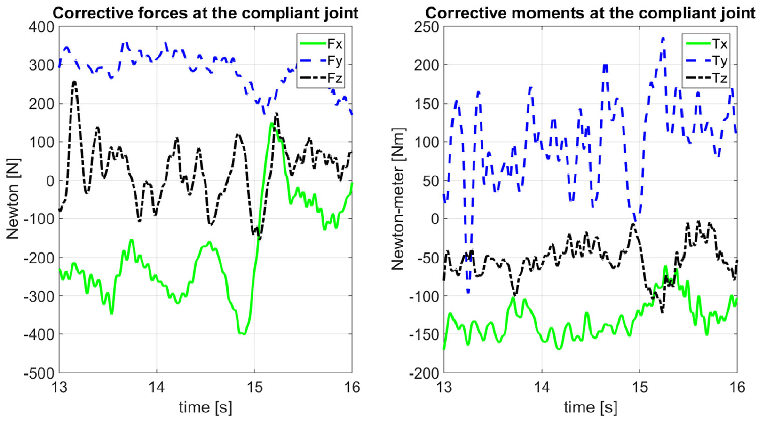
Controller corrective forces and moments at the compliant joint during braking maneuver between 75 and 35 km/h.

Figure 24.

Controller corrective forces and moments at the compliant joint during the 30 km/h speed bump.

As seen in all three figures, the spring-damper controller applies significant forces and moments during the simulation to compensate errors from the vehicle actual motion. Indeed, peak efforts of around 1200 N were recorded in the y-axis and 1000 Nm in the z-axis for the DLC, 400 N in the z-axis and 235 Nm in the y-axis for the braking and 1800 N in the z-axis and 900 Nm in the y-axis for the speed bump. The corrective effort amplitudes were greatly dependent on the principal load axis of the maneuver. In the DLC, the translational lateral (y-axis) and angular yaw (z-axis) directions of the vehicle are greatly stressed during this maneuver. In the braking maneuver, the translational longitudinal (x-axis) and the angular pitch (y-axis) were predominantly stressed. In the bump maneuvers, the translational vertical (z-axis) and angular pitch (y-axis) were predominantly stressed as well. Moreover, the amplitudes of the efforts seemed to be also dependent on the variation rate of the input loads generated by the maneuvers. Indeed, for the DLC and speed bump maneuvers, in which the loads amplitudes changed more rapidly than during the braking maneuver, higher corrective forces and moment amplitudes were required.

Discussion

The goal of this study was to predict frame loads during dynamic maneuvers using a hybrid (semi analytical) simulation based on the CCRP method. To assess the accuracy of the method, the semi analytical data were compared with experimental data and full analytical data based on the same MBD model. In general, good results were observed with the semi analytical method, correlating over 90% on the DLC and braking maneuvers, which are slow dynamics. The semi analytical method even slightly outperformed the full analytical in these cases. For faster dynamics, such as the speed bump, both simulations started to show some limitations with correlation values dropping in the order of 50%–80%. The semi analytical model showed better accuracy than the full analytical one in this case. This was expected since the frequency content of the WFTs (1000 Hz) is much higher than the frequency content of the MF-Tyre (8 Hz) used in the full analytical simulation. The advantage of using the semi analytical method for predicting high-speed dynamics could have been smaller or even negligible if a more suitable tire model had been chosen for this type of maneuver. Performing the same study with a tire model designed for NVH analysis such as the MF-Swift,²⁴ CDTire,²⁵ or FTire²⁶ would be an interesting avenue for future work. Still, the WFTs actual bandwidth is higher than most tire models currently available which should make hybrid simulations more advantageous for high frequency inputs.

One reason that might explain the limitations in high dynamic cases is the rigidly fixed pilot assumption. Indeed, even though the test pilot was asked to remain as still as possible, upper body reaction was noticeable during faster dynamic maneuvers (such as the speed bump), therefore limiting the upper body pitch motion amplitude. Indeed, during the experimental speed bump test, when the pilot hit the speed bump, his arms, and upper body absorbed the impact while during both types of simulations, the pilot was propelled forward creating a high-pitching moment and adding inertia in the pitch and roll directions. This phenomenon seems to impact the rear behavior of the vehicle more, as rear suspension displacement and strain values in the swing arm are, again, more impacted during the speed bump maneuver (Figures 20 (right) and 21 (right)).

The lower accuracy at higher frequencies was expected on the full analytical simulations as the MF-Tyre model is only correlated under 8 Hz. A higher degree of correlation was expected for higher frequencies with the semi analytical simulations. The lower than expected correlation is partly explained by the bandwidth difference between the IMU and the WFTs. Indeed, the sampling frequency of the IMU (200 Hz, filtered with an ideal filter at 50 Hz) is 20 times less than the WFTs (1000 Hz). The filtering of the IMU data was needed in order to smooth the curves used as input to the simulation. Indeed, the resolution of the IMU, especially for the speed data, was too coarse for the solver thus creating unwanted behavior. By filtering the curves used as inputs, the data used by the solver is smoother, but this also limits the frequency content of the IMU. Since the semi analytical model receives both data as inputs, the IMU data as positioning information and the WFTs as road inputs applied at the spindle, there are discrepancies between the two inputs during high frequency maneuvers since the IMU signals frequency content is lower than the WFTs signals. Indeed, the frame motion caused by the WFT inputs is of higher frequency than what the IMU can record. Still, the spring-damper controller uses the IMU data as the translational and angular orientation reference and, therefore, applies significant corrective forces and moments to the vehicle’s frame during the maneuvers. This is particularly apparent on the corrective forces and moments applied by the controller during the DLC and speed bump maneuver in which the variation rates of the loads at the wheel spindle are high. The corrective efforts impact the accuracy of the semi analytical simulations. An IMU with a higher bandwidth and a better resolution would be recommended to further enhance the semi analytical results.

Conclusion

In this study, semi analytical simulations, using the CCRP method, were used to predict suspension displacements and strains in the flexible parts of a vehicle model. Results were compared with full analytical simulations and experimental data. The model was validated using three maneuvers that loaded the vehicle both laterally, longitudinally and vertically with moderate to high intensity. Semi analytical simulations were generally equal or slightly better at predicting the experimental data than the full analytical simulations. Both methods showed comparable accuracy with coefficients of determination over 90% for low dynamic maneuvers. For faster dynamic maneuvers, the prediction accuracy was generally lower with semi analytical simulations showing better results. Thus, in the later stages of a vehicle development project, before a first prototype is ready to ride, implementing hybrid MBD analysis (semi-analytical) in the development process provides valuable information to the design team.

Footnotes

Handling Editor: James Baldwin

Declaration of conflicting interests

The author(s) declared no potential conflicts of interest with respect to the research, authorship, and/or publication of this article.

Funding

The author(s) disclosed receipt of the following financial support for the research, authorship, and/or publication of this article: This work was supported by PRIMA under grant R13-13-008 and by the Natural Science and Engineering Research Council (NSERC) under grant RDCPJ 500450 – 16.

ORCID iD

Carl Blanchette

References

Schudt

Kodali

Hong

H-J

, et al. Supplementation of measured vehicle road loads to study vehicle configuration changes. SAE technical paper 2005-01-1403, 2005.

Zhang

Liu

Zhang

, et al. Component load predication from wheel force transducer measurements. SAE technical paper 2011-01-0737, 2011.

Johannesson

Speckert

Dressler

, et al. Guide to load analysis for durability in vehicle engineering. Chichester: Wiley, 2013.

Chen

J-S

Hwang

H-Y

. All terrain vehicle flexible multibody dynamic simulation for fatigue prediction. Adv Mech Eng 2013; 5: 1–6.

Cossalter

Lot

Massaro

. An advanced multibody code for handling and stability analysis of motorcycles. Meccanica 2011; 46: 943–958.

Balamurugan

Srinivasan

. Tracked vehicle performance evaluation using multi body dynamics. Def Sci J 2017; 67: 476–480.

Braccesi

Cianetti

Landi

. Random loads fatigue: the use of spectral methods within multibody simulation. In: ASME 2005 International design engineering technical conferences and computers and information in engineering conference, Long Beach, California, 24–28 September 2005, pp.1735–1745.

Shoberg

Wallace

. A Triaxial automotive wheel force and moment transducer. SAE technical paper 750049, 1975.

Lin

Wang

Zhang

, et al. Research on the online initial value calibration method for the wheel force transducer. Sens J IEEE 2015; 15: 1043–1054.

10.

Bäcker

Langthaler

Olbrich

, et al. The hybrid road approach for durability loads prediction. SAE technical paper 2005-01-0628, 2005.

11.

Da Cruz

Do Espírito Santo

De Oliveira

. A semi-analytical method to generate load cases for CAE durability using virtual vehicle prototypes. SAE technical paper 2003-01-3667, 2003.

12.

Joubert

Boisvert

Blanchette

, et al. Frame loads accuracy assessment of semianalytical multibody dynamic simulation methods of a recreational vehicle. Multibody Syst Dyn 2020; 50: 189–209.

13.

Tebbe

Chidambaram

Kline

, et al. Chassis loads prediction using measurements as input to an unconstrained multi-body dynamics model. SAE technical paper 2006-01-0992, 2006.

14.

Pacejka

Bakker

. The magic formula tyre model. Veh Syst Dyn 1992; 21(Suppl. 1): 1–18.

15.

Lugner

Pacejka

Plöchl

. Recent advances in tyre models and testing procedures. Veh Syst Dyn 2005; 43(6–7): 413–436.

16.

ISO/TC 22/SC 33 C. ISO 3888-2:2011 Passenger cars—Test track for a severe lane-change manoeuvre—Part 2: Obstacle avoidance. Vernier, Geneva: International Organization for Standardization, 2011.

17.

Kammer

Baker

. Comparison of the Craig-Bampton and residual flexibility methods of substructure representation. In: Collection of technical papers – AIAA/ASME/ASCE/AHS/ASC structures, structural dynamics and materials conference, Orlando, Florida, 15–17 Aprill 1985, pp.699–706.

18.

Wenzel

Burnham

Blundell

, et al. Dual extended Kalman filter for vehicle state and parameter estimation. Veh Syst Dyn 2006; 44: 153–171.

19.

Jin

Yang

, et al. Online estimation ofinertial parameter for lightweight electric vehicle using dual unscented Kalman filter approach. IET Intell Transp Syst 2020; 14: 412–422.

20.

Antonov

Fehn

Kugi

. Unscented Kalman filter for vehicle state estimation. Veh Syst Dyn 2011; 49: 1497–1520.

21.

Winter

. Anthropometry. In: Biomechanics and motor control of human movement. Hoboken, NJ: John Wiley & Sons, Ltd, 2009, pp.82–106.

22.

Ramachandran

Vasudevan

Brahma

, et al. Estimation of mass moment of inertia of human body, when bending forward, for the design of a self-transfer robotic facility. J Eng Sci Technol 2016; 11: 166–176.

23.

Carrère

. Statistiques descriptives: Théorie et applications, ZI des Vouillands, Fontaine: PUG– Presses universitaires de Grenoble; 2015.

24.

Schmeitz

AJC

Besselink

IJM

Jansen

STH

. TNO MF-SWIFT. Veh Syst Dyn 2007; 45(Suppl. 1): 121–137.

25.

Gallrein

Bäcker

. CDTire: a tire model for comfort and durability applications. Veh Syst Dyn 2007; 45(Suppl. 1): 69–77.

26.

Gipser

. FTire – the tire simulation model for all applications related to vehicle dynamics. Veh Syst Dyn 2007; 45(Suppl. 1): 139–151.

Dynamic input loads evaluation of a recreational vehicle frame using multibody dynamics hybrid modeling validated with experimental and full analytical modeling data

Abstract

Keywords

Introduction

Methodology

Vehicle models and general testing protocol

Instrumented vehicle

Maneuvers

Double lane change (DLC)

Braking

Speed bump

MBD vehicle model

Weight and Inertia calibration of the MBD model

Full analytical simulation

Semi analytical (hybrid) simulation

Results

Double lane change (DLC)

Braking

Speed bump

Corrective forces and moments applied by the controller

Discussion

Conclusion

Footnotes

Declaration of conflicting interests

Funding

ORCID iD

References