Sage Journals: Discover world-class research

Abstract

This study designed a crawling mechanism that can solve the measurement problems of slender and needle pipes by detecting the heating vertical needle pipe, which is greatly applied in the petrochemical and refinery industry. The robot’s walking system uses a single driven wheel to stick on the way, with a scissor-hand structure to adapt to changes in diameter between 50 and 90 mm. This study lists the dynamic analysis equation of the robot, thereby obtaining the optimum range of Angle α between the horizontal line and the center line of the main driving wheel and the main clamping wheel. Moreover, the study uses multi-body dynamics simulation software for dynamics simulation analysis. Results indicate that the crawling system has the advantages of anti-deviation, can adapt to different pipe diameters and has a simple structure.

Keywords

Pipe robot crawling pipe simulation diameter adaptation

Introduction

At present, various pipelines are increasingly used in the petrochemical industry.^1,2 For example, the heating furnace, which is widely used in petrochemical and refining plants, often uses the heating furnace pipe to transfer heat.^3,4 When the heating furnace pipe used for a long time is damaged, the cost of pipe maintenance or replacement is high. Therefore, the heating furnace pipe should be cleaned and monitored regularly, and this process requires manual labor, where the working environment is bad and the work efficiency is low.^5,6 The research and application of the crawling robot technology outside the pipe can free people from the harsh environment and will greatly improve the working environment of workers and increase productivity.

At present, studies on the robot outside the pipe at home and abroad are limited. The existing structures for the crawling mechanism outside the pipe wall are as follows: wheel type,⁷ pneumatic peristaltic type,⁸ inchworm type,⁹ and multi-joint type structure.¹⁰ The furnace pipe wall climbing robot must run smoothly and continuously for pipe wall detection. The scissor-hand driving wheel walking mechanism is adopted in the design scheme of the robot for inspecting row furnace pipe. The design principle is derived from the foot buckle used by electricians to climb poles, and the robot uses its own gravity and driving force for stable and continuous crawling.¹¹ Owing to its own structural characteristics, its load capacity is small, but the mechanism has the advantages of simple structure, flexible walking, and stable operation. Thus, this robot is suitable for the detection of heating vertical needle pipe.

The outside needle pipe climbing robot system is mainly composed of four parts, namely, axial walking system, centering system, sensor detection system, and control system. Figure 1 shows the schematic diagram of the outside needle pipe climbing robot system. When the detection robot works, the axial walking system driven by the walking motor is equipped with sensors to make a continuous or intermittent straight walking movement along the vertical pipe, which can realize the continuous or intermittent measurement of the pipe through the sensors.

Figure 1.

Schematic diagram of the outside needle pipe climbing robot.

Structure design of the outside needle pipe climbing robot

The diameter of the furnace pipe in the heating furnace is generally 50–90 mm, and the furnace pipe is distributed in a vertical row, and the distance between the horizontal row pipes is approximately 63 mm. Three problems should be considered when designing the driving wheel of the crawling mechanism for the furnace pipe: (a) can be extended and clamped within the distance of 63 mm between the pipes; (b) easy to install and disassemble; and (c) can adapt to pipe diameter changes in the range of 50–90 mm.

The pipe climbing robot studied in this paper needs to crawl under the condition of small pipe diameter and pipe string spacing. Because the distance between two adjacent pipes is very small, it is impossible to arrange the attachment and climbing mechanism in the circumferential direction of the pipe string. In order to prevent the robot from sliding down the vertical pipe surface, the robot must maintain sufficient clamping force (positive pressure) between the robot and the pipe surface to generate sufficient friction and to be able to resist overturning. The robot structure adopts scissor-driven wheel-type walking mechanism. The design principle is derived from the foot buckle used by human when climbing trees or poles, which makes full use of the weight of human body to realize stable and continuous climbing.

The robot uses a single motor to drive the wheel type walking system. Then, the axial walking system uses a stepping motor to drive the driving wheel through a bevel gear to make continuous or intermittent linear movement along the pipeline axis. The overall layout is shown in Figure 1. The walking system of the crawling robot is mainly composed of two parts, namely, (a) motor, bevel gear, and driving wheel; and (b) driven wheel and pipe diameter adjusting part. The motor is fixed on the base through the support plate of the motor, and the motor shaft is connected with the bevel gear by the key through the bearing seat. The radial torque of the motor is converted into the driving force of the axial driving wheel through 90° engagement of the bevel gear.

The main driving mechanism is composed of the main driving wheel, a pair of 90° engaging bevel gears and a DC servo motor, as shown in Figure 2.

Figure 2.

Schematic diagram of the main driving mechanism: (a) front view and (b) top view.

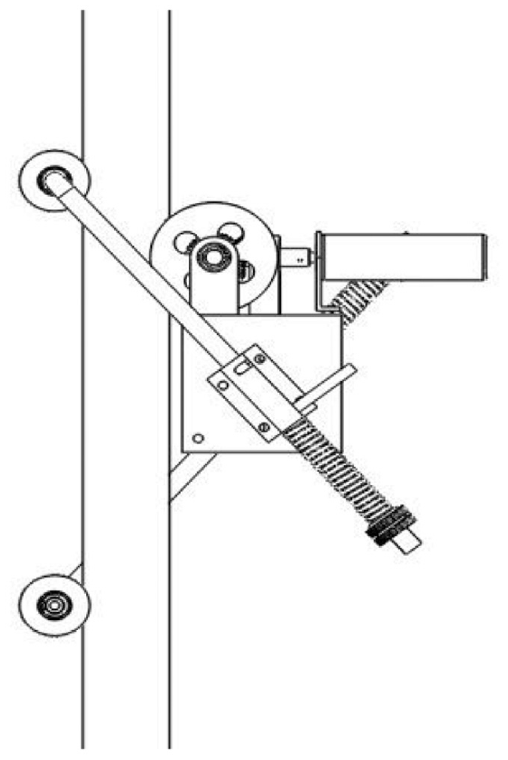
Figure 3 depicts the design of the driven wheel mechanism, which adopts the upper and lower symmetric scissor-hand structure.

Figure 3.

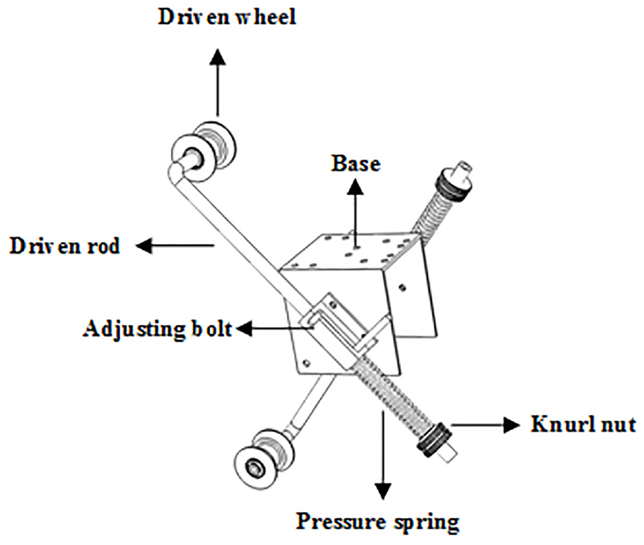
Schematic diagram of the driven wheel mechanism.

The driven wheel mechanism is mainly composed of a base, adjusting bolt, driven rod, driven wheel, pressure spring, and others. The driven wheel is connected to the driven rod through bearings to reduce friction with the pipe under test. The driven wheel and the driving wheel are arcs shaped to increase the contact area with the pipe and reduce wear. During installation, first, we insert the long vertical end of the driven rod into the adjusting bolt and fix it with a bolt. Then, we load the pressure spring into the driven rod and fix it with a knurl nut, as shown in Figure 3. After the initial installation is completed, we adjust the position of the knurled nut according to the pipe diameter to be tested. Considering the action of the pressure spring, the bolt is at the left end of the adjusting bolt. We screw the bolt into the short-range track of the adjusting bolt so that the driven wheel is in a vertical state. We repeat the process of the driven wheel on the other side. In this way, the driven wheels on the left and right sides of the robot can easily enter into the gap between the row pipes, solving the problem that the robot is not easy to operate. When the robot is fixed, the bolt is screwed into the long-range track of the adjusting bolt, and the driven wheel is clamped to the pipe under the action of the pressure spring. The assembly and disassembly processes are simple and can be fully realized by a single operator.

As for the problem of how to adapt to the change of pipe diameter in the range of 50–90 mm, according to the mechanical analysis in Chapter 3, Angle α between the horizontal line and the center line of the main driving wheel and the main clamping wheel has an effect on the range of the crawler pipe diameter. Therefore, α can be changed to adapt to different pipe diameters. With the increase of α, the diameter of traceable pipe decreases. Table 8 in Section 4.2 lists the corresponding relationships of several Angle α adaptations to furnace pipe diameters. In addition, in Section 3.2, we also designed an Angle α adjusting mechanism, as shown in Figure 7.

Robot walking system analysis

Simplified model static analysis

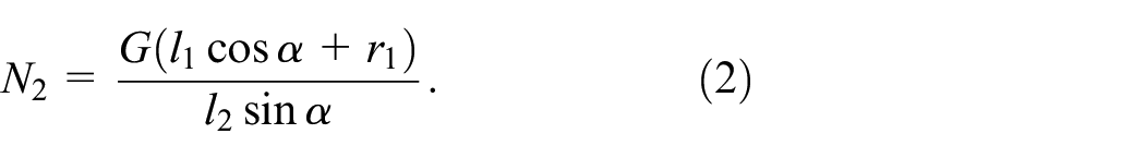
Through the simulation analysis, we observe that the size of the included Angle α between the horizontal line and the center line of the main driving wheel and the main clamping wheel not only affects the range of the crawling pipe diameter but also directly affects the clamping force between the robot and the crawling pipe wall. The mechanical model of the robot is simplified, and its statics is analyzed, as shown in Figure 4.

Figure 4.

Simplified diagram of the foot buckle mechanical model.

Amongst them:

a – the distance between the center of gravity and the point of contact between the main driving wheel and the string, mm;

b – the distance between the main driving wheel and the string contact point and the main clamping wheel and the string contact point, mm;

d – crawling string diameter, which is a constant in this analysis, mm;

α– the angle between the horizontal line and the center line of the main driving wheel and the main clamping wheel;

l ₁– distance from center of gravity to center of the main driving wheel, mm;

l ₂– distance between center of the main driving wheel and center of the main clamp wheel, mm;

G– the robot gravity, N;

Wheels 1 and 2 are the main driving wheel and the main clamping wheel, respectively;

N ₁ and N₂ are the positive pressure (clamping force) on the wall of the main driving wheel and the main clamping wheel, respectively, N;

F ₁ and F₂ are, respectively, the friction between the two wheels and the pipe wall, N;

r ₁ and r₂ are the main driving wheel radius and the main clamping wheel radius, respectively, mm.

Firstly, the models of the main driving wheel and main clamping wheel are simplified, and the effect of the second clamping wheel is temporarily ignored, and the simplified model of foot buckle is changed. Supposing that the robot crawls upward at a constant speed, the total center of gravity of the robot shifts to the rear. As wheel 2 is a driven wheel, F₂ is its driving force, and F₂ is the rolling friction force, Moreover, the torque at the center of wheel 2 is balanced with the friction resistance torque at the clamping wheel 2 axis: $F_{2} r_{2} = M_{2}$ . In the state of constant motion, according to the force and torque balance of the robot, the torque of point C (the tangent point between the main driving wheel 1 and the pipe string) is taken to obtain the following:

G (l_{1} \cos α + r_{1}) = F_{2} d + N_{2} l_{2} \sin α .

(1)

Therefore, $N_{2} = \frac{G (l_{1} \cos α + r_{1}) - \frac{M_{2}}{r_{2}} d}{l_{2} \sin α}$ .

As bearings are used at the shaft of clamping wheel 2, the torque M₂ is relatively small and can be ignored in engineering. Therefore, the contact pressure of the clamping wheel can be simplified as follows:

N_{2} = \frac{G (l_{1} \cos α + r_{1})}{l_{2} \sin α} .

(2)

When the robot is stationary on the pipe string, and the friction force of the pipe wall on both wheels is upward, the condition for preventing sliding is as follows:

F_{1} + F_{2} \geq G .

(3)

Considering that F₁ is the sliding friction between the wheel and the pipe wall, $F_{2} r_{2} = M_{2}$ , and then,

N_{1} f + \frac{M_{2}}{r_{2}} \geq G,

(4)

where f is the sliding friction coefficient between the roller and the pipe wall.

Therefore, when the robot crawled on the pipe wall, the torque M₂ was relatively small and could be ignored in engineering. Therefore, the condition for the robot not to skid is the following:

N_{1} \geq \frac{G}{f} .

(5)

According to the static equilibrium, N₁ = N₂. Therefore, by substituting equation (2) to equation (5), the condition under which the robot can crawl without skidding can be obtained as follows:

N_{1} = N_{2} = \frac{G (l_{1} \cos α + r_{1})}{l_{2} \sin α} \geq \frac{G}{f} .

(6)

Alternately,

l_{1} \geq l_{2} \frac{1}{f} \tan α - \frac{r_{1}}{\cos α}

(7)

In equation (7), $α = \arccos (\frac{r_{1} + r_{2} + d}{l_{2}})$

According to equation (6), if the distance of l₁ from the center of gravity center to the center of the main driving wheel and the radius r₁ of the main driving wheel and the weight of the robot G remain unchanged, then the positive pressure (clamping force) between the robot and the pipe string and whether the robot can crawl on the pipe string are all related to Angle α.

Dynamic analysis of a scissor-hand model

For the scissor-shaped clamping mechanism, Figure 5 depicts the force analysis. The positive pressure $N'_{1}$ on wheel 1 due to the existence of spring force can be analyzed separately. Then, pressure N₁ in the simplified model analysis above is superimposed as the actual positive pressure of the main driving wheel 1 to generate the driving force.

Figure 5.

Simplified diagram of the scissor-hand mechanical model.

We take the connecting rod of wheels 1 and 2 for analysis and the torque at point O₁ to write the balanced equation:

N'_{2} \cdot l_{2} \sin α - F_{s} l_{3} \cos α = 0

(8)

To: $N'_{2} = \frac{F_{s} l_{3} \cos α}{l_{2} \sin α}$

The scissor mechanism is automatically tightened by the spring force and wheels 2 and 3 symmetrical position. Thus, $N'_{2} = N'_{3}$ ;

N'_{1} = N'_{3} + N'_{2} = 2 N'_{2} = \frac{2 F_{s} l_{3} \cos α}{l_{2} \sin α} .

(9)

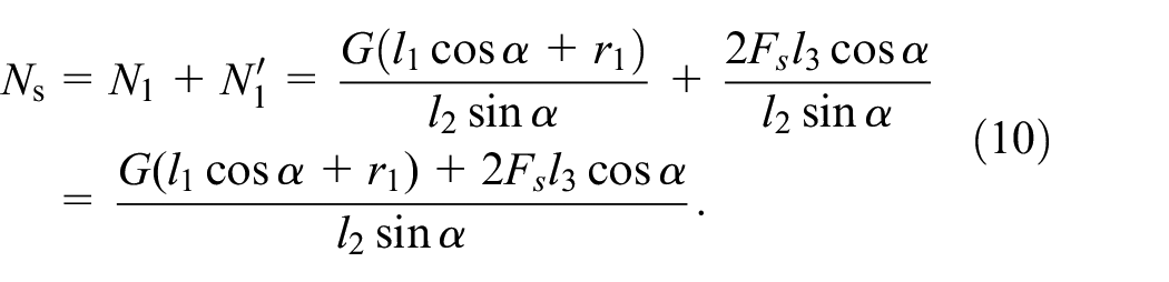
Therefore, the total pressure of wheel 1 on the pipe wall is as follows:

\begin{matrix} N_{s} = N_{1} + N'_{1} = \frac{G (l_{1} \cos α + r_{1})}{l_{2} \sin α} + \frac{2 F_{s} l_{3} \cos α}{l_{2} \sin α} \\ = \frac{G (l_{1} \cos α + r_{1}) + 2 F_{s} l_{3} \cos α}{l_{2} \sin α} . \end{matrix}

(10)

Then, the conditions for the robot not to skid and crawl are as follows:

N_{s} = \frac{G (l_{1} \cos α + r_{1}) + 2 F_{s} l_{3} \cos α}{l_{2} \sin α} \geq \frac{G}{f} .

(11)

Given that l₂ is the distance between two wheels, we can set $l_{1} = u l_{2}$ and $l_{3} = v l_{2}$ and substitute it into:

N_{s} = \frac{G (u \cos α + r_{1} / l_{2}) + 2 v F_{s} \cos α}{\sin α} \geq \frac{G}{f} .

(12)

In equation (12), $α = \arccos (\frac{r_{1} + r_{2} + d}{l_{2}})$ .

Equation (12) shows that when u and v are constant, the Angle α is smaller, the positive pressure between the robot and the pipe string is greater, and meeting the self-locking condition of the robot is easier. Therefore, Angle α should be smaller. By comparing equations (6) and (12), the scissor-hand structure can obtain a greater clamping force than the foot buckle structure.

Therefore, what is the appropriate range for Angle α?

When Angle α becomes smaller, the positive pressure of the driving wheel on the pipe wall increases according to equation (12), that is:

\begin{matrix} N_{s} = \frac{G (l_{1} \cos α + r_{1}) + 2 F_{s} l_{3} \cos α}{l_{2} \sin α} \\ = \frac{G (u \cos α + r_{1} / l_{2}) + 2 v F_{s} \cos α}{\sin α} . \end{matrix}

(13)

N_s is going to increase.

To determine N_s, enough value should be assured to avoid robots from skidding. Moreover, if the value is too large, then the running resistance will unnecessarily increase. As N_s is influenced by u, v, r₁, and α, the best design to make these parameters have an impact on the N_s is not particularly sensitive. Otherwise, variable working conditions (e.g. the pipe diameter change or having a small bending pipe) will cause drastic changes to positive pressure N_s, which is not conducive to the stability of the robot’s adaptability and crawling pipeline. Based on equation (13), we can draw the relationship curves between N_s and α, and u and v and determine the region with relatively gentle curve changes as the selection point of our parameters.

If α and v are constant, then, according to equation (13), N_s and u change linearly. In the same way, if α and u are constant, then N_s and v will change linearly. Only the relationship between N_s and α is a nonlinear change, so we should look for the best range value of α through their relationship curve.

Let G = 60 N, u = 1.1, v = 0.7, F_s = 20 N, r₁ = 30 mm, l₂ = 60 mm. We use excel list to determine N_s, and Figure 6 shows the graph.

Figure 6.

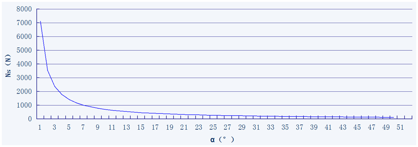
Relationship between Angle α and clamping force.

Figure 6 shows that when Angle α is very small, the positive pressure is quite large. N_s and pressure change with α. That is, if the working point is selected in this area, then Angle α causes a slight change during the process of the crawling robot due to reasons, such as deformation of the wall. Angle α can cause great changes of positive pressure, which changes the driving force of the driving wheel, thereby inevitably producing unstable situations, such as vibration. Furthermore, Angle α can even cause a lack of driving force. If α is set to a value beyond 20°, N_s changes smoothly with α, but the positive pressure generated is relatively small and the driving force is also small.

To obtain greater positive pressure and better adaptability, the parameters near the inflection point of the curve can be selected. For example, when α = 5°, N_s = 1418 N, and when α = 7°, N_s = 1011 N. If robots use a polyurethane rubber wheel, according to the literature “Study on the Friction Characteristics of Polyurethane for the Friction Liner of Hoisting,”¹² the coefficient of friction between wheels and pipe wall can increase to more than 0.53. Moreover, the static friction coefficient of 45 steel is approximately 0.38, friction is approximately 0.45 and the coefficient of friction also increased with the increase of friction velocity increases. In another literature, “Study on the Law of Friction and Wear of Polyurethane,”¹³ the sliding friction coefficient is 0.5. Therefore, to keep the robot from slipping, the friction coefficient should be calculated according to the static friction, so f_st = 0.38.

In the case of such model parameters, if the mass of the robot is m and the static friction coefficient is set to 0.38, then the F_st that the robot can produce is equal to F_st = N_s × f_st. Moreover, the safety factor to ensure that the robot does not slip in the static state needs to meet $S = \frac{F_{st}}{G_{robot}} \geq 1.5$ . When the robot accelerates and climbs upward, the friction of the required driving wheel can also meet the driving force, which is greater than that of the robot.

Based on the results of mechanical analysis and the size of the robot structure model, the selected Angle α can be adjusted within the range of 9°–20°, leaving a certain crawling safety factor. We select the appropriate value to determine α according to different pipe diameters and pipe string surface roughness.

From the above analysis, the size of Angle α for the robot to crawl on the string and self-locking is crucial. To easily adjust Angle α, we have designed the following mechanism: can be connected to the base and the adjusting bolt, and can more easily change the horizontal line of the pitch Angle and the clamping rod. Figure 7(a) shows the installation position of the adjusting bolt of the main clamping wheel side on the base. Then, Figure 7(b) depicts the installation position of the adjusting bolt of the second clamping wheel side on the base, and Figure 7(c) illustrates the 3D schematic diagram.

Figure 7.

Angle α regulating mechanism design.

Analysis of robot driving force

Analysis of rolling frictional resistance

The rolling friction coefficient is the resistance coefficient δ of the wheel when rolling, and the product of this coefficient and the positive pressure is the rolling friction resistance torque. The rolling resistance torque divided by the wheel radius is the driving force acting on the axle. Figures 8 and 9 are respectively the rolling friction torque diagram and the simplified diagram of mechanics of the robot.

Figure 8.

Rolling friction torque diagram.

Figure 9.

Simplified diagram of mechanics.

Rolling friction resistance torque = rolling friction coefficient × positive pressure, that is, $M_{m} = N \cdot δ_{r}$ .

The driving force necessary to overcome the rolling friction resistance torque is $F_{m} = \frac{M_{m}}{r} = \frac{N \cdot δ_{r}}{r}$ .

Then, the driving force required to overcome the rolling friction resistance torque of the driving wheel when it crawls is as follows:

F_{m 1} = \frac{M_{m 1}}{r_{1}} = \frac{N_{A} \cdot δ_{r}}{r_{1}} .

(14)

The driving force required to overcome the rolling friction resistance torque when crawling from the driven wheel 2 is as follows:

F_{m 2} = \frac{M_{m 2}}{r_{2}} = \frac{N_{B} \cdot δ_{r}}{r_{2}} .

(15)

In equation (15), $N_{B} = \frac{F_{2} \cos γ'}{(\frac{l_{BC}}{l_{AB}} \frac{\cos α}{\sin γ} \cos γ + 2 \sin α + \frac{l_{BC}}{l_{AB}} \sin α)} \frac{l_{BC}}{l_{AB}} \frac{\cos α}{\sin γ}$ .

The driving force required to overcome the rolling friction resistance torque when crawling from the driven wheel 3 is shown below:

F_{m 3} = \frac{M_{m 3}}{r_{3}} = \frac{N_{C} \cdot δ_{r}}{r_{3}} .

(16)

In equation (16), $N_{C} = \frac{F_{3}}{\cos β}$ .

Driving force analysis

We suppose that the mass of the robot is m kg, and the acceleration of startup is a m/s², which is 0.3 m/s². Then, the driving friction required by the driving wheel is as follows:

F_{q} = mg + ma + F_{m 1} + F_{m 2} + F_{m 3},

(17)

where F_m is the rolling friction resistance of the driving wheel and the two clamping wheels.

F_m is the resistance of the three wheels, ignoring the resistance torque between the wheel and the bearing. F_m is mainly the resistance along the pipe wall generated by the rolling resistance torque of the driving wheel and the two clamping wheels, as shown in equation (18).

F_{m} = F_{m 1} + F_{m 2} + F_{m 3},

(18)

F_{m} = \frac{N_{A} \times δ_{g}}{r_{1}} + \frac{N_{B} \times δ_{g}}{r_{2}} + \frac{N_{C} \times δ_{g}}{r_{3}},

(19)

where wheels 2 and 3 have the same diameter; δ_g is the rolling resistance coefficient; N_A = N_B + N_C; mass m, 10 kg, gravity G; f is the friction coefficient of the clamping wheel against the pipe wall, set as 0.2.

Considering that the clamping wheel is a U-shaped grooved wheel, the equivalent Angle of the current main driving wheel is $θ$ , which is 84.8°. Then, the equivalent friction coefficient is as follows:

f_{Δ} = \frac{f}{\sin \frac{θ}{2}} = \frac{f}{\sin \frac{84 . 8^{°}}{2}} = 1.48 f = 1.48 \times 0.2 = 0.296

The static friction force between the main driving wheel and the pipe wall serves as the crawling force of the robot, which mainly overcomes the gravity of the vertical crawling robot itself. Thus, the robot gravity can be divided by the equivalent friction coefficient to estimate the clamping force between the main driving wheel and the pipe wall, as shown in the following formula:

N_{A} \approx \frac{G}{f_{Δ}} = \frac{10 \times 9.8}{0.296} = 331 N .

According to equation (19), F_m can be estimated to be approximately 11.6 N.

Then, the driving force of wheel climbing is calculated as follows:

F_{q} = mg + ma + F_{m} = 101 + F_{m} = 112.6 N .

In this way, the positive pressure of wheel 1 on the pipe wall can be modified again:

N_{A} \geq \frac{F_{q}}{f_{Δ}} \approx \frac{112.6}{0.296} = 380 N .

The friction coefficient between the robot crawling wheel and the pipe wall has a great influence on the positive pressure between the driving wheel 1 and the pipe wall. The friction coefficient of 0.2 can be selected according to the more severe conditions.

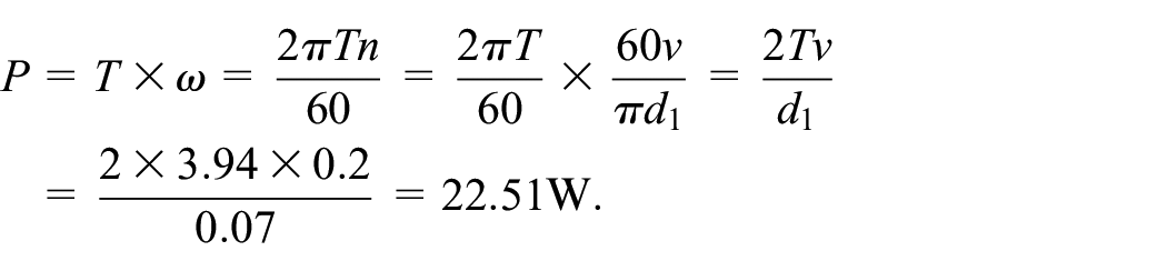
The radius of the driving wheel is r₁ = 35 mm, and then, the torque of the driving wheel shaft is shown below:

T_{1} = F_{q} \times r_{1} = 112.6 \times 0.035 = 3.94 N \cdot m .

In terms of the speed of the driving wheel, the fastest upward speed of the robot is 0.2 m/s, and then, the power at the wheel is as follows:

\begin{matrix} P = T \times ω = \frac{2 π Tn}{60} = \frac{2 π T}{60} \times \frac{60 v}{π d_{1}} = \frac{2 Tv}{d_{1}} \\ = \frac{2 \times 3.94 \times 0.2}{0.07} = 22.51 W . \end{matrix}

ADAMS dynamics simulation analysis

From the mechanical analysis, the robot dynamics was analyzed by using Adams/View software. The rationality of the robot design was verified by studying the self-locking condition of the robot, the influence of the change of Angle α on the clamping force and the ability to cross the obstacle after heating deformation of the pipe.

Simulation analysis of robot self-locking performance

In the simulation test, the real working conditions were simulated, and the spring preload of 100, 50, 40, 35, and 30 N was applied to the spring. Then, the contact force between the driving wheel and the clamping wheel and the pipe was measured. Figure 10 shows the contact between the wheel and the pipe.

Figure 10.

Relative position of wheels.

Tables 1 to 4 show the simulation values of the contact force between the wheel and the string surface after applying different spring pressures, which can maintain the self-locking state. The simulation time is 20 s, and the step length is 0.02.

Table 1.

Contact force value when spring preload is 100 N.

Position of contact force	F_x (N)	F_y (N)	F_z (N)
Driving wheels
Left	403	441	−55.8
Right	420	−461	−58.4
Clamping wheel
Down (second)	−139.5	3.6	6.7
Up (main)	−684	15.5	9.41

Table 2.

Contact force value when spring preload is 50 N.

Position of contact force	F_x (N)	F_y (N)	F_z (N)
Driving wheels
Left	205	225	−56.5
Right	221.3	−243.3	−60.1
Clamping wheel
Down (second)	−64.4	3.5	4.5
Up (main)	−362.3	14.4	8

Table 3.

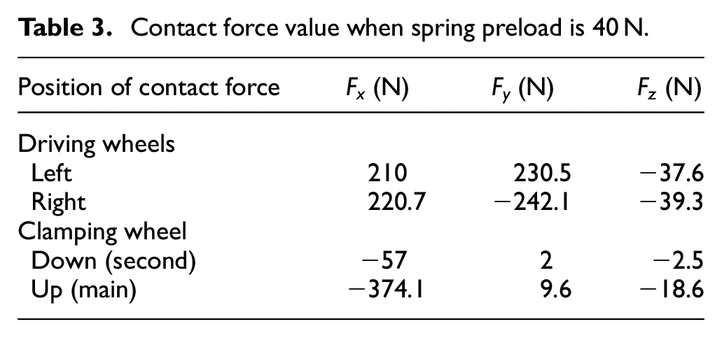
Contact force value when spring preload is 40 N.

Position of contact force	F_x (N)	F_y (N)	F_z (N)
Driving wheels
Left	210	230.5	−37.6
Right	220.7	−242.1	−39.3
Clamping wheel
Down (second)	−57	2	−2.5
Up (main)	−374.1	9.6	−18.6

Table 4.

Contact force value when spring preload is 35 N.

Position of contact force	F_x (N)	F_y (N)	F_z (N)
Driving wheels
Left	183.7	201.5	−39
Right	199	−218.3	−40.8
Clamping wheel
Down (second)	−48.4	1.5	−1.7
Up (main)	−334.5	13.8	−16.5

Given that the driving wheel is a U-shaped wheel, the positive pressure between the driving wheel and the pipe in the XY plane is $F_{N} = \sqrt{{F_{x}}^{2} + {F_{y}}^{2}}$ . In addition, the expression of the maximum static friction force should be F_st = μ × F_N. As the above states can satisfy the self-locking of the robot, and the robot is in a state of balance, the measured data in the table show that the sum of the forces received by the driving wheel and the clamping wheel in the X and Y directions, respectively, is approximately 0. As the direction of gravity is the positive direction of Z-axis, Tables 1 to 4 show that the sum of the component forces in the z direction of the driving wheel and the clamping wheel is F_z = F_st = −G. Moreover, the positive pressure of the driving wheel and pipe wall on the left and right sides is larger. Given that the gravity of the robot itself plays a major role in self-locking, Tables 1 to 4 show that $F_{N, up} = \sqrt{{F_{x}}^{2} + {F_{y}}^{2}}$ of the upper clamping wheel is the largest.

When the 30 N preloading force is applied from the spring on the clamping rod, the Adams simulation animation shows that the robot has a sliding phenomenon. Table 5 shows the measured contact force and friction force.

Table 5.

Contact force value when spring preload is 30 N.

Position of contact force	F_x (N)	F_y (N)	F_z (N)
Driving wheels
Left	155.6	172	−36.3
Right	156.2	−173.6	−46.4
Clamping wheel
Down (second)	−39.2	1.1	0
Up (main)	−276.5	1.1	−5.7

Table 5 shows that the sum of the frictional force in the Z direction between the driving wheel, the clamping wheel and the pipe wall is less than 90 N < G, and thus, sliding occurs.

From the above analysis, after setting the constraints, contact and fixation between components and selecting the appropriate friction coefficient, the Adams software is used to simulate that the spring preload should be set at least 35 N to maintain the self-locking state of the robot when the maximum allowable Angle α of the mechanism is 30°. Figures 11 and 12 show the spring damping and amplitude diagrams of the contact force between the left driving wheel and the pipe wall in Adams when the spring preload is set to 35 N.

Figure 11.

Damping diagram of spring.

Figure 12.

Amplitude diagram of the contact force between the left driving wheel and the pipe wall.

Simulation analysis of the influence of Angle α change on clamping force

In the simulation test, the real working conditions were simulated, and the main clamping mechanism was locked after obtaining an appropriate Angle α. Angle α was set at 20° and 9° for simulation, as shown in Figure 13.

Figure 13.

Schematic diagram of Angle α.

To make the driving speed of the robot reach 0.2 m/s, the driving wheel diameter should be 70 mm. According to v = ω·r, the driving speed is set as ω = 5.714 rad/s in Adams. To obtain sufficient initial acceleration when the robot crawled vertically, a large spring preload should be set, and 50 N preload force should be applied to the slave clamp spring. The driving wheel is a U-shaped wheel, so the positive pressure with the pipeline in the XY plane is $F_{N} = \sqrt{{F_{x}}^{2} + {F_{y}}^{2}}$ . The simulation time is 20 s, and the step length is 0.02.

After setting, we initially measure the positive pressure of the pipeline and the robot when Angle α is 20°, as shown in Table 6.

Table 6.

Contact force measurements when Angle α = 20°.

Position of contact force	F_x (N)	F_y (N)	F_z (N)	F_N (N)	F_Nx (N)
Driving wheels
Left	332.6	421.8	−44.9	537.2	677.1
Right	344.5	−433	−60.8	553.3
Clamping wheel
Down (second)	−64.5	2.5	1.3	64.5	−64.5
Up (main)	−613.1	9.6	9.8	613.2	−613.1

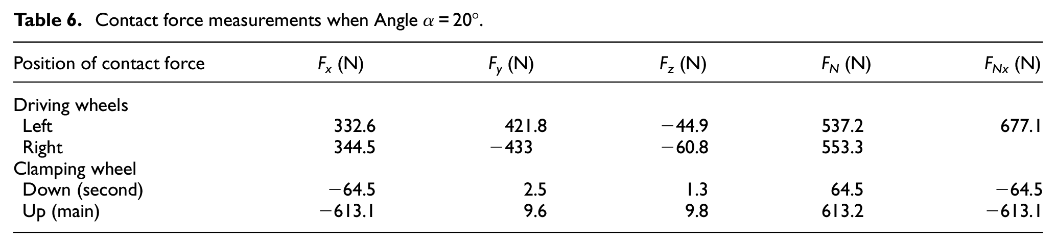
Figure 14 depicts the driving torque diagram when Angle α is 20°.

Figure 14.

Driving torque diagram of Angle α = 20°.

Figure 14 shows that under the set conditions, the average driving torque required for robot climbing is approximately 3.871 N m when Angle α between the horizontal line and the central line of the driving wheel and the main clamping wheel is set to 20°. The driving torque is consistent with the above-deduced results, which further verifies the accuracy of the simulation.

Then, we measure the positive pressure of the pipeline and the robot when Angle α = 9°, as shown in Table 7.

Table 7.

Contact force measurements when Angle α = 9°.

Position of contact force	F_x (N)	F_y (N)	F_z (N)	F_N (N)	F_Nx (N)
Driving wheels
Left	612.7	685.8	−44.8	919.6	1210.2
Right	597.5	−664.2	−62.1	893.4
Clamping wheel
Down(second)	−60.9	−2.3	0.5	60.9	−60.9
Up(main)	−1150.1	−18.2	7.0	1150.2	−1150.1

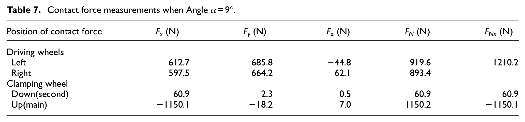
Figure 15 shows the driving torque diagram when the Angle α is 9°.

Figure 15.

Driving torque diagram of Angle α = 9°.

Figure 15 depicts that under the set conditions, the average driving torque required for robot climbing is approximately 4.132 N m when Angle α between the horizontal line and the central line of the driving wheel and the main clamping wheel is set to 9°.

By comparing the terms F_N and F_Nx in Tables 6 and 7, evidently, when Angle α is set to 9°, the positive pressure between either the driving wheel or the main clamping wheel and the pipe string in the XY plane is greater than that when Angle α is set to 20°. The simulation results further verify the effect of Angle α on the positive pressure between the robot and the pipe wall. That is, if Angle α is small, then the positive pressure is great. By comparing Figures 14 and 15, when Angle α is 20°, the driving torque required by the robot is less than that when Angle α is 9°.

Crawling simulation analysis of expansion coarsening furnace pipe

The heating furnace pipe will be coarsened locally after being heated for a long time. The robot needs to adapt to the crawling of the local diameter coarsened pipe. After simulating real working conditions, the main clamping mechanism is locked after obtaining the appropriate Angle α. The driving speed of the robot reaches 0.2 m/s. The simulation time was set to 9 s and the step length was set to 0.1 for simulation, as shown in Figure 16.

Figure 16.

Simulation diagram of furnace pipe coarsening expansion climbing: (a) expanding and thickening furnace tube and (b) crawling posture diagram.

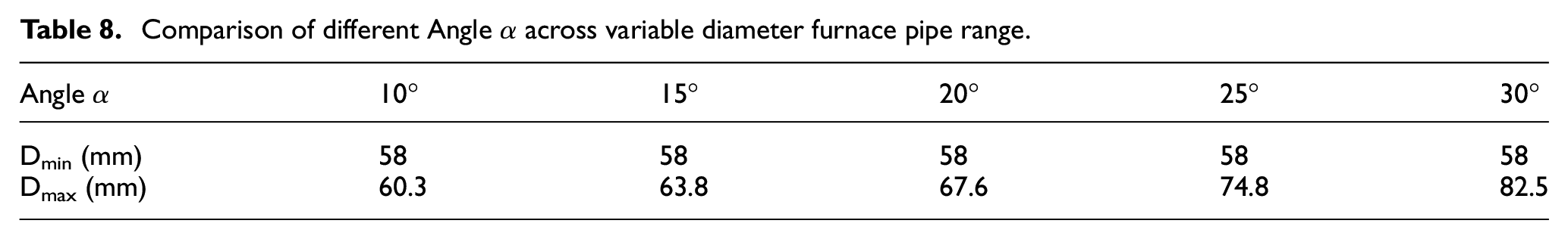
The simulation animation shows that when the main clamping mechanism is locked, a different Angle α has a different diameter of the coarsened furnace pipe that the robot can cross. Table 8 shows the corresponding relationship between different angles α that can span the coarsening furnace pipe.

Table 8.

Comparison of different Angle α across variable diameter furnace pipe range.

Angle α	10°	15°	20°	25°	30°
D_min (mm)	58	58	58	58	58
D_max (mm)	60.3	63.8	67.6	74.8	82.5

The normal pipe diameter of 58 mm under common working conditions was selected. The maximum diameter of heating expansion coarsening was 61 mm, the deformation zone had a 60 mm transition and the maximum expansion zone of 62 mm continued to be 1000 mm long for analysis. In the simulation, Angle α was set to 25°, and the spring force variation curve, driving torque curve and crawling line velocity curve of the main driving wheel were simulated and analyzed in the expansion zone.

Figure 17(a) illustrates that when the robot runs to approximately 4 s, the robot starts to enter the expansion zone of the furnace pipe. Moreover, the diameter of the crawling pipe becomes larger, which can be seen from the simulation curve of the spring pressure. Owing to the locking of the main clamping mechanism, when the robot’s main driving wheel enters the expansion zone, Angle α decreases to accommodate the large diameter of the pipe crawl. At this time, the elongation spring from the second clamping rod is compressed due to the limitation of the robot structure. When the robot enters the expansion zone, the spring force increases.

Figure 17.

Simulation curve of expansion furnace pipe climbing: (a) spring pressure diagram, (b) driving torque diagram, and (c) driving wheel speed diagram.

Then, Figure 17(b) shows that the average driving torque required by the robot when crawling in the deformed pipeline is 3.913 N m, and the maximum driving torque is 8.660 N m. The selected motor blocking torque is much larger than this peak value.

Moreover, Figure 17(c) depicts that the crawling speed of the robot is relatively stable, which is suitable for crawling across the expansion and deformation pipe of the heating furnace pipe.

Figure 18 shows the change of the contact force between the driving wheel and the pipeline when crossing the expansive deformed pipeline. As shown in the simulation graph, when the robot driving wheel crawls into the expansion area of the pipeline at approximately 4 s, the contact force increases, with a maximum peak value of 1192.9 N and an average value of 449.4 N. The size of the contact force can meet the crawling requirements of the expansion zone pipe climbing robot.

Figure 18.

Contact force diagram of the driving wheel of the expansion furnace pipe.

Conclusion

To sum up, the designed clamping mechanism and pipe diameter adjusting mechanism consider the requirements of pipe diameter adjustment, small clearance, row pipe, and so on, and the disassembly is simple. This mechanism can fully realize a single-person operation. The design can well solve the three problems faced by the axial walking system for small clearance row pipe to be tested when it crawls. The design of the outside needle pipe climbing robot has the advantages of a simple structure, light and flexible, stable operation and strong adaptability, which can meet the requirements of continuous and stable measurement. Figure 19 shows the prototype of this design.

Figure 19.

Prototype of this design.

The simulation results of the virtual prototype show that the design scheme is reasonable and feasible. This finding is of general guiding significance to the dynamic analysis of the simplified model of the crawling mechanism. Moreover, the research provides a reference for the design of similar walking mechanisms.

Footnotes

Acknowledgements

We thank Prof. Fujun He (School of Mechanical Science and Engineering, Northeast Petroleum University) for the help in conducting this experiment. We acknowledge useful discussions with Dr. Baojin Wang.

Handling editor: James Baldwin

Declaration of conflicting interests

The author(s) declared no potential conflicts of interest with respect to the research, authorship, and/or publication of this article.

Funding

The author(s) disclosed receipt of the following financial support for the research, authorship, and/or publication of this article: National Natural Science Foundation of China (51675011); Science and Technology Planning Project of Guangdong Province (2017A010102022).

ORCID iD

Zihua Zhang

References

Dai

Zhang

. SPC ROBOT: a novel pipe-climbing robot with spiral extending of coupled differential. In: 2017 IEEE international conference on robotics and biomimetics, Macau SAR, China, 5–8 December 2017, pp.1088–1093.

Yoshioka

Marumoto

Gotoh

. Electromagnetic inspection method of carburization depth inside and outside of heating furnace steel tube. Int J Appl Electromagn Mech 2019; 59: 1283–1290.

Liao

, et al. Experimental study of the effect of a radiant tube on the temperature distribution in a horizontal heating furnace. Appl Therm Eng 2017; 113: 1–7.

Feng

Ruan

Liu

, et al. The research of heating furnace with heavy oil desander. In: 2011 2nd International conference on advances in energy engineering, Bangkok, Thailand, 27 December 2011, pp.674–680.

Gotoh

Ishida

. Evaluation of electromagnetic inspection of outer side defect on small diameter and thick steel tube with steel support using 3-D nonlinear FEM. IEEE Trans Magn 2014; 50: 1–4.

Xie

Liu

Kang

, et al. Fully 3D-printed modular pipe-climbing robot. IEEE Robot Autom Lett 2021; 6: 462–469.

Takeda

Shimoyama

. Analysis of the vertical driving performance of multiple connected pipe-climbing microrobots with magnetic wheels. Micromachines 2019; 10: 524.

Tanise

Kishi

Yamazaki

, et al. High-speed response of the pneumatic actuator used in a peristaltic crawling robot inspecting long-distance gas pipes. In: 2016 IEEE international conference on advanced intelligent mechatronics, Banff, AB, Canada, 12–15 July 2016, pp.1234–1239.

Khan

Chuthong

, et al. iCrawl: an inchworm-inspired crawling robot. IEEE Access 2020; 8: 200655–200668.

10.

Yaqub

Ali

Usman

, et al. A spiral curve gait design for a modular snake robot moving on a pipe. Int J Control Autom Syst 2019; 17: 2565–2573.

11.

Zhao

Liu

, et al. Design and analysis of a climbing robot for pylon maintenance. Ind Rob 2018; 45: 206–219.

12.

Fuyan

Dongsheng

Xiangdong

. Study on the friction characteristics of polyurethane for the friction liner of hoisting. Lubr Eng 2000: 33–34+60.

13.

Yao

Yang

. Study on the law of friction and wear of polyurethane. J Hebei Univ Sci Technol 2000; 21: 86–88.