Design of optimal flow concentrator for vertical-axis wind turbines using computational fluid dynamics,artificial neural networks and genetic algorithm

Abstract

Wind energy extraction is one of the fastest developing engineering branches today. Number of installed wind turbines is constantly increasing. Appropriate solutions for urban environments are quiet, structurally simple and affordable small-scale vertical-axis wind turbines (VAWTs). Due to small efficiency, particularly in low and variable winds, main topic here is development of optimal flow concentrator that locally augments wind velocity, facilitates turbine start and increases generated power. Conceptual design was performed by combining finite volume method and artificial intelligence (AI). Smaller set of computational results (velocity profiles induced by existence of different concentrators in flow field) was used for creation, training and validation of several artificial neural networks. Multi-objective optimization of concentrator geometric parameters was realized through coupling of generated neural networks with genetic algorithm. Final solution from the acquired Pareto set is studied in more detail. Resulting computed velocity field is illustrated. Aerodynamic performances of small-scale VAWT with and without optimal flow concentrator are estimated and compared. The performed research demonstrates that, with use of flow concentrator, average increase in wind speed of 20%–25% can be expected. It also proves that contemporary AI techniques can significantly facilitate and accelerate design processes in the field of wind engineering.

Introduction

Due to some of the pressing issues of modern society, that include climate change, global warming, pollution, etc, the extraction of wind energy is one of the fastest developing engineering fields today. As an answer to the growing energy needs, the number of installed wind turbines is constantly increasing. International Renewable Energy Agency (IRENA) ¹ reports that the capacity of installed wind power reached nearly 564 GW in 2018 worldwide. Furthermore, European Union acknowledged reaching a share of at least 32% of renewable energy till 2030 as a binding target. ² One possibility to make better use of wind energy resources in urban and densely populated areas is to install many small-scale wind turbines. Many computational studies deal with this topic, for example, Arteaga-Lopez et al. ³ employ computational fluid dynamics (CFD) approach on building-mounted wind turbines while Stathopoulos et al. ⁴ accentuate both potentials and challenges of urban wind energy.

Generally, it is possible to classify wind turbines as either horizontal-axis (HAWTs) or vertical-axis (VAWTs) according to the direction of their rotation axis. VAWTs are much less employed, but aerodynamically very interesting structures, particularly in starting regimes. ⁵ Their main advantages are decreased noise, operability in lower and changeable wind speeds as well as reasonable price. However, due to their inherently smaller efficiency than HAWTs, approximately 0.15–0.35 in comparison to 0.40–0.50 in HAWTs as demonstrated,^6–9 they are the topic of many optimization studies. Some additional problems might include operation in Earth’s boundary layer and vortex trail of surrounding objects. Possible solutions and improvements are continually being offered, both for the drag- and lift-type architectures. For the drag-type Savonius turbine Alom and Saha ⁶ provide a thorough review of power augmentation techniques. Alizadeh et al. ¹⁰ use a simple barrier to deviate the flow. For the lift-type VAWTs, adjustments range from the modifications to the wind turbine structure itself in the form of blade adaptation as demonstrated by Preen and Bull ¹¹ and Baghdadi et al. ⁸ who investigated supershapes and morphing blades, respectively, or airfoil optimization as considered by De Tavernier et al. ¹² to the addition of the separate elements that would serve as flow directors or concentrators and whose main role is to locally amplify flow velocity. For example, De Santoli et al. ¹³ investigated a VAWT with a surrounding linear, convergent duct. Similarly, Cho et al.^14,15 investigated both numerically and experimentally the design parameters of towers that could improve VAWT performance. For more details and examples, Wong et al. ¹⁶ provide a good overview of the tried VAWT performance enhancements.

Bearing in mind the thought that if not adapted to the complex wind environment, a VAWT might not be a successful energy converter, a novel optimal flow concentrator (specifically designed for a particular geometry operating in local winds) is proposed. In order to achieve this, several requests have to be met: omni-directional operability must be preserved, flow concentrator should induce accelerated sub-sonic flow and the construction should be the simplest possible. These demands lead to an axisymmetric geometry converging from the windward side (i.e. all the sides since wind blows from all directions). Therefore, the proposed concentrator consists of two half-ellipsoids, lower and upper, as illustrated in Figure 1. Such a design is characterized by compactness, simplicity, and omnidirectional operability. Apart from the possible boost of local velocity and generated power, if designed properly, this innovative concept also leads to an easier start of the VAWT, expansion of its operational range as well as an increase in the number of working hours. To accomplish this, the geometric parameters of the flow concentrator should be optimized with respect to the global dimensions of the planned wind turbine as well as the wind conditions at the chosen location.

Figure 1.

Isometric view of a H-rotor with the flow concentrator.

Regardless of the method, optimization usually implies performing a large number of repetitive actions which makes it unsuitable to be coupled with CFD techniques since they still generally require significant computational resources. And this is where artificial neural networks (ANNs) come in as a perfect tool for the estimation of highly non-linear functions in multidimensional space. Here, they can facilitate the prediction of the velocity profiles of interest to the VAWT. Although they are not often utilized in the fields of aerodynamics and rotational machinery there are some examples. Mortazavi et al. ⁹ used ANN and multi-objective genetic algorithm (MOGA) to obtain the set of optimal HAWT airfoils. Mohammadi et al. ⁷ used computational intelligence to study the relations between the parameters of the Savonius rotor and to perform its single-objective GA optimization. Kuppers et al. ¹⁷ also coupled CFD with ANN in order to optimize vertical-axis Kirsten–Boeing turbine. Finally, the authors also previously used ANNs to control boundary layers around foils in linear cascades. ¹⁸

The paper is organized as follows: since this is primarily a computational study, adopted numerical approaches are firstly validated in the next section. Chapter 3 provides a description of the parameterized concentrator model that is used in flow computations covered in section 4. Performed simulations of the spatial, steady flow field surrounding the concentrator, assuming incompressible, viscous fluid were conducted by finite volume method (FVM). After performing a sufficient number of computations, several ANNs were created, trained and validated and this procedure is described in section 5. Multi-objective GA optimization is explained in section 6. Finally, obtained results, conclusions and experience are summarized.

Validation of the computational approaches

Since the performed study includes both flows around flow concentrators as well as around VAWT rotors, the validation of the employed CFD models was also realized in two phases. In the first step, simulating unsteady flows around a VAWT rotor was investigated, in order to ensure that its aerodynamic performances can be computationally estimated with satisfactory accuracy.

Computation of rotational flows around a VAWT rotor

As previously mentioned, simulating flows around VAWTs still presents quite a challenge since numerous flow phenomena might appear such as flow and vortex separation, dynamic stall, etc. Numerous simpler numerical models have been tried and used but the most usual approach today assumes 3D, unsteady, turbulent flow around a moving rotor, solved by finite volume method (FVM). However, it still does not provide completely reliable results, particularly in cases of higher rotor solidities which are the most convenient solutions for urban environment, and should be validated through comparison with available experimental data.

The model and its results obtained in an open-air wind tunnel testing used for verification of the adopted numerical set-up are provided by Bravo et al. ¹⁹ The 3-bladed H-rotor (B = 3) has radius R = 1.25 m (and diameter D = 2.5 m), length L = 3 m and blade chord c = 0.4 m resulting in rotor reference area A = DL =  7.5 m², and solidity σ = Bc/D = 0.48 (that can be considered high). The blade has constant profile along its length, shaped like a symmetric NACA 0015 airfoil, with a blunt trailing edge.

Flow simulations, together with all the pre- and post-processing, were fully realized in the engineering software package ANSYS.

Outer, stationary part of the computational domain is shaped like a cuboid and extends −6D and +18D fore and aft of the rotor axis, ±9D to the sides and ±4D along the vertical axis. Inner, rotational part is in a form of a hollow cylinder encompassing the blades. Other wind turbine elements (e.g. struts, mast, and base) were neglected.

Computational mesh is hybrid unstructured, meaning it primarily contains tetrahedral cells but also 25 layers of prismatic cells encompassing the blade walls to ensure an appropriate value of dimensionless wall distance y⁺ < 5. It is refined in the vicinity of the interface boundary as well as leading and trailing edges of the blades. It numbers approximately 1.7 million elements (which is not particularly fine but is appropriate for this optimization study).

Flow computations by means of numerically solving fundamental flow equations (mass and momentum conservation equations as well as additional transport equations of turbulence quantities) are performed in ANSYS FLUENT. The flow around the wind turbine is considered as spatial, transient, incompressible and viscous (i.e. turbulent). The effects of rotor rotation are simulated by sliding-mesh approach, where in every time-step Δt, the inner zone is actually rotated for a small angular increment Δψ.

Unsteady Reynolds-averaged Navier-Stokes (URANS) equations were closed by a two-equation k-ω SST turbulence model, ²⁰ based on Boussinesq hypothesis, that provides good results and is often employed in the engineering problems from the field of computational aerodynamics. It presents a combination of standard k-ω model near the walls and k-ε in the outer layer. As observed by Menter et al., ²⁰ its features (modifications) make it more accurate and reliable for flows including airfoils, adverse pressure gradient flows, etc.

Different operating conditions, that is, tip-speed ratios λ = RΩ/V_o, are accomplished by various combinations of undisturbed wind velocity V_o assigned along the inlet boundary and angular speed of the rotor Ω. Zero gauge pressure Δp = 0 Pa is defined at the outlet surface. No-slip boundary conditions are defined at walls that are, in this case, rotational.

Pressure-based solver is employed with SIMPLEC pressure-velocity coupling scheme. All spatial derivatives are approximated by second order schemes, and temporal derivatives by first order scheme. One time-step corresponds to Δψ = 2°, while the number of iterations per time-step is 10. The computations were performed until reaching periodic convergence of torque coefficient C_Q = Q/(0.5ρV_o²RA), which usually required at least three revolutions. Computed averaged torque coefficients (per revolution) were then used for the estimation of wind turbine power coefficient C_P = C_Qλ.

By looking at Figure 2(a) certain discrepancies between the two data sets can be observed. Computed maximal power coefficient C_P of approximately 0.265 is slightly smaller than the measured values from the range [0.25, 0.30] (these changes depend on the actual wind speed V_o). Also, computed optimal tip-speed ratio λ of about 1.85 is somewhat higher than the measured value of approximately 1.6. However, since these differences remain below 15% and are on the safety side (i.e. the real turbine performs better), numerical results can be considered quite satisfactory and the defined set-up may also be used for the optimization purposes.

Figure 2.

Comparison of measured and computed: (a) VAWT power coefficient curves and (b) sphere drag coefficient.

Computation of (unsteady and transitional) flows around a sphere

In the second step, flows around a smooth sphere were simulated. This standard geometry (of high relative thickness) was chosen because it has been extensively experimentally investigated in the past while being comparable to the assumed flow concentrator geometry (both are rotational bodies derived from second order curves). However, although standard in shape, it is by no means simple to compute. The flow is highly dependent on Reynolds number (Re), surface roughness and free stream turbulence intensity. In the range of Re that are expected around the flow concentrator, that is, [10⁵, 10⁶], the flow transits from laminar to turbulent (when the drag coefficient drops significantly), and with further increase in speed, there is massive, highly unsteady flow separation (due to the alternating generation of vortices from the pressure and suction sides) that leads to a new escalation in drag.

Here, the radius of the sphere is R = 1 m. Shape and dimensions of the outer computational domain are similar to the ones described in section 4.1. Cuboid domain extends −9R and +18R fore and aft, and ±9R in the two remaining directions. The sphere center coincides with the coordinate beginning. Again, the mesh is hybrid unstructured, with a thick layer of prismatic cells encompassing the walls and producing dimensionless wall distance lower than 1. Computational grid is refined around the sphere and numbers approximately 920,000 cells. More details on its specific features are provided in section 4.2.

Since this flow case is used to validate the numerical approach applied to flow concentrator geometry, computational set-up is similar to the one described in section 4.3 with the important difference that these flows were mostly solved as transitional and unsteady. Uniform velocity profile, resulting in 10⁵ < Re < 10⁶, was assumed along the inlet boundary. Time-step used in computations was 0.02 s. In cases of highly unsteady and oscillating flow, it was necessary to simulate periods of time ranging 30–100 s.

The comparison of experimentally and numerically obtained results is presented in Figure 2(b). A precise approximation of the experimental data used for model validation was taken from Almedeij. ²¹ Error-bar of computed points for higher values of Re denotes the amplitudes in drag coefficient oscillating character. Again, although there are discrepancies between the two sets of data (caused by the effects of walls in wind tunnels, roughness of sphere surface and turbulence levels in free stream), the overall trend of the computed drag coefficient curve seems well captured. The effects of Reynolds number are clearly present. Since flows around spheres are particularly complex (unsteady and transitional), the results obtained on a relatively course mesh can be considered satisfactory for preliminary study purposes that involve optimization (that is the main topic of this research). Furthermore, the surface gradients of half-ellipsoids that are considered in continuation are considerably lower than those of a sphere, so less dynamic flows can be expected (that include much weaker vortex shedding as well as quasi-steady flow states).

Definition of the parameterized concentrator model

Since the flow concentrator should be designed in accordance with the wind turbine, it is first necessary to make some assumptions regarding the dimensions and vertical position of the rotor. Here, a scaled-down (by factor 2) version of the 3-bladed model described in the previous section is used. Its diameter, blade length and chord are D = 1.25 m, L = 1.5 m, and c = 0.2 m, respectively, as illustrated in Figure 3, while the distance of its central point to the ground equals 2.75 m. The flow concentrator and the wind turbine rotor are positioned coaxially.

Figure 3.

Four geometric parameters of the concentrator and its position in space.

The two parts of the concentrator, lower and upper, are assumed in the shape of half-ellipsoids. Being axisymmetric, they are completely determined by four input parameters: semi-major and semi-minor axes of the lower part, a₂ and b₂ respectively, and semi-major and semi-minor axes of the upper part, a₁ and b₁ respectively. The distances between the wind turbine and the concentrator are kept the same for all considered concentrator models, meaning that the position of the wind turbine is fixed in space while the concentrator parts are positioned accordingly (y-coordinates of the lower and upper co-vertices are 2 m and 3.5 m, respectively) as illustrated in Figure 3.

Different concentrator geometries were achieved by diverse combinations of input parameters. The values of the semi-major axes were allowed to take values from the range 1.0 m ≤ a ≤ 2.2 m, and semi-minor axes b from the set [0.3 m, 1.2 m], Figure 3. In order to generate a valid and well-founded basis for the development of ANNs, 300 miscellaneous models were numerically computed. Output parameters in the form of minimum, average and maximum speed (that would serve to define goal functions for the ensuing optimization) along a characteristic cross-section that is, a line located 0.75 m downstream from the rotational axis were extracted from the computed accelerated velocity fields.

Flow simulation

Again, as with validation cases, all flow simulations were realized in ANSYS. The following subsections provide details of the adopted computational approach.

Parameterized geometry

All necessary 3D models were created in ANSYS DesignModeler to facilitate the definition of input parameters. The computational domain is defined in the same manner as the previously described outer, stationary zone from the validation study, that is, extending −6D and +18D fore and aft, ±9D to the sides and ±4D along the vertical axis measured from the assumed rotational axis. The lower end of the wind turbine is supposed to be placed at the height of 2 m, and its upper end should reach 3.5 m (since the planned height of the wind turbine is 1.5 m). These points coincide with the co-vertices of the lower and upper half-ellipsoids.

The two concentrator parts (completely defined by the four input parameters a₁, a₂, b₁, b₂) are cut-out from the fluid zone. The boundaries of the computational domain are: inlet, outlet, wall_ground, wall_1 (upper part of the concentrator) and wall_2 (lower part of the concentrator).

Grid generation

Families of similar, hybrid unstructured meshes are generated using ANSYS Meshing. Each mesh is both globally and locally refined. Cell size along the walls of the concentrator is set to 100 mm. The boundary layer encompassing the two parts of the concentrator contains N = 30 layers of prismatic cells, with growth rate of q = 1.2 and first layer thickness of y₁ = 0.1 mm. The other boundary layer along the ground also contains 30 layers of prismatic cells, with growth rate of 1.2 but with the increased first layer thickness of y₁ = 1 mm.

As a result, each generated grid contains approximately 800,000 cells. This level of fineness was adopted after a grid convergence study as quite satisfactory for a repeated number of numerical simulations. A representative example is illustrated in Figure 4.

Figure 4.

A detail of one of the generated meshes.

Numerical set-up

Again, spatial, incompressible, turbulent but in this case steady flow around the flow concentrator is simulated using ANSYS FLUENT by solving RANS equations closed by k-ω SST turbulence model. ²⁰

In order to simulate the flow in the Earth’s boundary layer as accurate as possible, height-dependent velocity profile is defined along the inlet boundary, Figure 5. Here, a power-law velocity profile is assumed where V(h) = V_ref(h/h_ref)^α. The reference wind speed at the reference height of h_ref = 10 m is V_ref = 5 m/s while the value of exponent α = 0.15 corresponds to terrain roughness class 2. Such a velocity profile implies that a velocity of approximately V_o = 4.12 m/s hits the assumed wind turbine’s central point as illustrated in Figure 5. This smaller wind velocity is purposely simulated to resemble urban environment. Zero gauge pressure is defined at the outlet. No-slip boundary conditions are assumed along all the walls.

Figure 5.

Profile of wind speed V(h) [m/s] defined along the inlet.

Since the flow was considered incompressible, again, the pressure-based solver with the SIMPLEC pressure-velocity coupling scheme were employed. To increase accuracy, all spatial derivatives were approximated by second order schemes. Computations were performed for 1000 iterations that is, until reaching the converged values of minimum, average and maximum speeds along the characteristic line located 0.75 m downstream from the rotational axis.

Results

The final results (used for both ANN formulation and subsequent optimization) are the same as the aforementioned convergence criteria. For each considered model, the values of minimum, average and maximum velocity along the characteristic line were registered. They were recorded as two distinct goal functions: average speed V_mean and min-to-max speed ratio V_min/V_max that serves to quantify the uniformity of the velocity field in the downstream part of the rotor that is generally more critical for VAWT performance.

Artificial neural networks (ANNs)

ANNs present a very suitable and often employed means for forecasting and modeling the behavior of complex nonlinear systems. Today, they are used for a large number of applications in many research fields. Some typical applications in aerospace include: flight simulations, control systems, autopilots, aircraft component behavior simulations, aircraft component fault detection, maintenance analysis, image/signal identification, processing, and compression. They were employed in this research because a fast and accurate prediction of output velocity profile based on four input geometric parameters was necessary for concentrator optimization, contrary to the solution of the nonlinear Navier-Stokes equations that takes up too much time.

Being inspired by biological nervous systems, ANNs comprise a net of intertwined artificial neurons which makes them suitable for replicating the performance of massive computational resources. Their architecture and performance are determined by the number of input and output parameters as well as the number of layers of neurons and connections between them.

A simplified description of the operation of a single artificial neuron j is illustrated in Figure 6(a). It can be explained as taking the sum of multiple inputs, scaled by weights w_ij, and bias b_j, and forming an output by applying an activation function f which is usually one of the sigmoid functions. Here, a hyperbolic tangent sigmoid function was used, f(x) = tanh x =  (e^x−e^−x)/(e^x+e^−x), for its main characteristics of continuity, smoothness, monotonicity, boundedness to range (−1, 1) and differentiability as illustrated in Figure 6(b).

Figure 6.

(a) Artificial multiple-input neuron and (b) hyperbolic tangent sigmoid function and its derivative.

Although several different ANNs were created, they all had the same architecture − a two-layer feed-forward network with 20 hidden neurons and two output neurons resulting in (4·20+20·2) + (1·20+1·2) = 142 initially unknown coefficients, 120 weights and 22 biases. It is depicted in Figure 7. Generally, a larger number of neurons in the hidden layer gives the network more flexibility, but can also lead to overfitting when the error of the training set appears to be very small, but the error of the new data being evaluated is actually large. The input vector contained the values of the four geometric concentrator parameters: a₂, a₁, b₂, and b₁, while the output vector stored the values of average velocity V_mean and min-to-max velocity ratio V_min/V_max.

Figure 7.

The adopted network architecture.

ANNs should be trained, that is, the weights and biases have to be determined, over a set of known events to provide sufficiently accurate estimations of untested scenarios. Here, 70% of the computed cases (210 models) were randomly chosen and used for training. Supervised learning by back-propagation iterative algorithm over the training set was applied as demonstrated by Hagan et al. ²² The remaining 30% were split into two equal halves (each containing 45 computed flow cases) and used for validation and testing, respectively. The validation dataset is used for the estimation of ANN’s performance during training and regulation of early stopping before overfitting, while the testing vectors are used as a further check and to provide insight into the final performances of the ANN (they do not affect the training).

The performances of generated ANNs can be quantified through the general parameters − the mean squared error which was approximately mse ≈ 1e⁻³ and the error standard deviation of roughly σ ≈ 0.01. This actually means that an approximate relative error in the estimation of average speed is below 1%, while the relative error in the estimation of min-to-max speed ratio is somewhat higher, but is still below 5%. In order to further reduce the prediction error, five different networks were created, trained and validated, and the final outputs were obtained by taking the average values of the five estimations for each considered input vector.

Multi-objective optimization by genetic algorithm

In order to find the most suitable concentrator geometry, a two-objective optimization by a heuristic, evolutionary genetic algorithm was performed.

Basics of GA

This is another algorithm derived from biological systems, but with the purpose of finding global optima of functions that are in some way tricky for example, non-linear, non-smooth, discontinuous, non-differentiable, stochastic, too complicated, etc. GAs simulate the course of natural selection and advancement through the developing generations of new entities. They involve some basic processes and behavior observed in groups of individuals such as favoritism, reproduction or mating, crossover and random mutation. Ever since their formulation, GAs have been extensively used in engineering applications. They are quite popular because: they enable the consideration of large numbers of input parameters, both continuous and discrete, do not require information of function derivatives, can search significant portions of design space in a single generation, can be parallelized or combined with multiple goal functions. A thorough review of contemporary wind turbine optimization techniques (among which GAs present a significant portion) and various studies is provided by Shourangiz-Haghighi et al. ²³

Although different variants exist as demonstrated, ²⁴ a general outline of GAs can be given. The process begins with the random generation of multitudinous initial population, where each individual is defined by an input vector − set of genes. This is followed by the cyclic repeating of:

• – estimating each individual of the population according to the chosen objectives or goals,

• – selecting the best individuals for mating,

• – producing children (by combining parents’ characteristics − crossover),

• – introducing random changes − mutations to a portion of the population to make sure that the process does not get stuck in local optima,

• – replacing the current with the newly formed population.

The process comes to a halt when the maximum number of generations is achieved or particular convergence criteria are met.

Implementation of MOGA

Same as with ANNs, each individual was described by the input vector containing the values of the four geometric concentrator parameters [a₂, a₁, b₂, b₁], while the output vector (used for selecting the best individuals) contained the values of average velocity and min-to-max velocity ratio [V_mean, V_min/V_max] estimated by ANNs. The MOGA optimization was performed over a population numbering 800 individuals, since the number of possible combinations of input parameters is practically infinite. The maximal number of generations was limited to 1000 which proved to be suitable for process convergence.

Estimating the goal functions of each individual results in a Pareto set that contains all equally good particles. From this set, 35% is randomly chosen and directly transferred to the next generation. The remainder of the new population is mostly formed by crossover (80%) and, to a smaller extent, mutation (20%).

Results and discussion

Two-criteria optimization

Optimization of the four basic geometric characteristics of the flow concentrator is executed on the basis of the estimated improvements in intensity and uniformity of the modified velocity field between the two concentrator parts. The obtained Pareto front, together with the computed cases (represented by dots), are illustrated in Figure 8. Marker shaped like the letter x presents the theoretical maximum, that is, the point whose values of abscissa and ordinate correspond to the maximal computed (by CFD) relative average speed and maximal min-to-max-velocity ratio, respectively. Since the final result of the performed optimization is actually a set of equally good optima, the choice of a single, definite solution is somewhat ambiguous. It mostly depends on the engineer designing the wind turbine, the initial requirements and the precedence of the chosen goal functions. For instance, if flow uniformity has the priority, one might single out Optimum 1, denoted by a triangle in Figure 8. In order to satisfy both goal functions, the final choice of the optimal solution can be made as the point closest to the theoretical maximum, that is, as Optimum 2 marked by a circle. Finally, if the highest value of average speed should be achieved, Optimum 3 designated by a square in Figure 8 could be selected. The obtained input and output parameters of the three chosen optima are listed in Table 1.

Figure 8.

Pareto front.

Table 1

Parameters of the chosen optima.

Optimum	a 2 [m]	a 1 [m]	b 2 [m]	b 1 [m]	V mean/Vo	V min/Vmax
1	1.71	1.51	0.61	1.20	1.173	0.995
2	2.20	1.70	0.84	1.20	1.223	0.950
3	2.20	2.20	0.90	1.20	1.281	0.889

As expected, the way to obtain the greatest average velocity is pretty straightforward. One should simply implement the largest flow concentrator since it produces the most considerable area contraction. On the other hand, if we also want flow uniformity or have special requirements regarding the incoming wind profile (that can be extremely irregular) several aspects should be simultaneously considered.

It is, however, possible to make some general conclusions by analyzing the set of obtained optima. While the optimal lower semi-major axis a₂ should be the greatest possible (≈2.2 m), the recommended value of the optimal upper semi-major axis a₁ should be smaller, that is, from the range [1.3 m, 1.9 m]. Also, while the optimal lower semi-minor axis b₂ may be around 0.8–0.9 m, the optimal upper semi-minor axis b₁ is almost uniformly distributed around 1.2 m. Overall, it can be concluded that the imposed velocity profile mostly requires elongated lower concentrator parts as well as chubby, more spherical upper parts.

Optimal solution

The coordinates [a₂, a₁, b₂, b₁] of the finally chosen optimum, that is, the point closest to the theoretical maximum, are [2.20 m, 1.70 m, 0.84 m, 1.20 m]. Detailed computational analysis of the optimal solution was also performed and the results are briefly presented qualitatively, by computed pressure, velocity and turbulence fields and flow visualizations by streamlines and vortex structures, and quantitatively by comparing the initial and improved velocity profiles.

Computed values of gauge pressure are depicted in Figure 9(a). As expected, the regions of the highest pressure correspond to the two frontal stagnation points (marked in red), while the lowest values appear between the two concentrator halves (marked in blue). Computed velocity field is illustrated in Figure 9(b) by colored streamlines originating from a line located upstream from the concentrator in the symmetry plane. Regions of locally accelerated flow (mostly between the two concentrator parts) are colored in red and orange. As a result of the notable asymmetry between the lower and upper concentrator part, the downstream flow seems more uniform than the upstream which was one of the optimization goals. It can also be seen that the flow between the two concentrator parts (where the wind turbine is supposed to be located) is even, accelerated and attached. The flow separation and vortex detachment only happen below, above and after the concentrator (empty regions) implying that no losses will be induced to the wind turbine by the flow concentrator.

Figure 9.

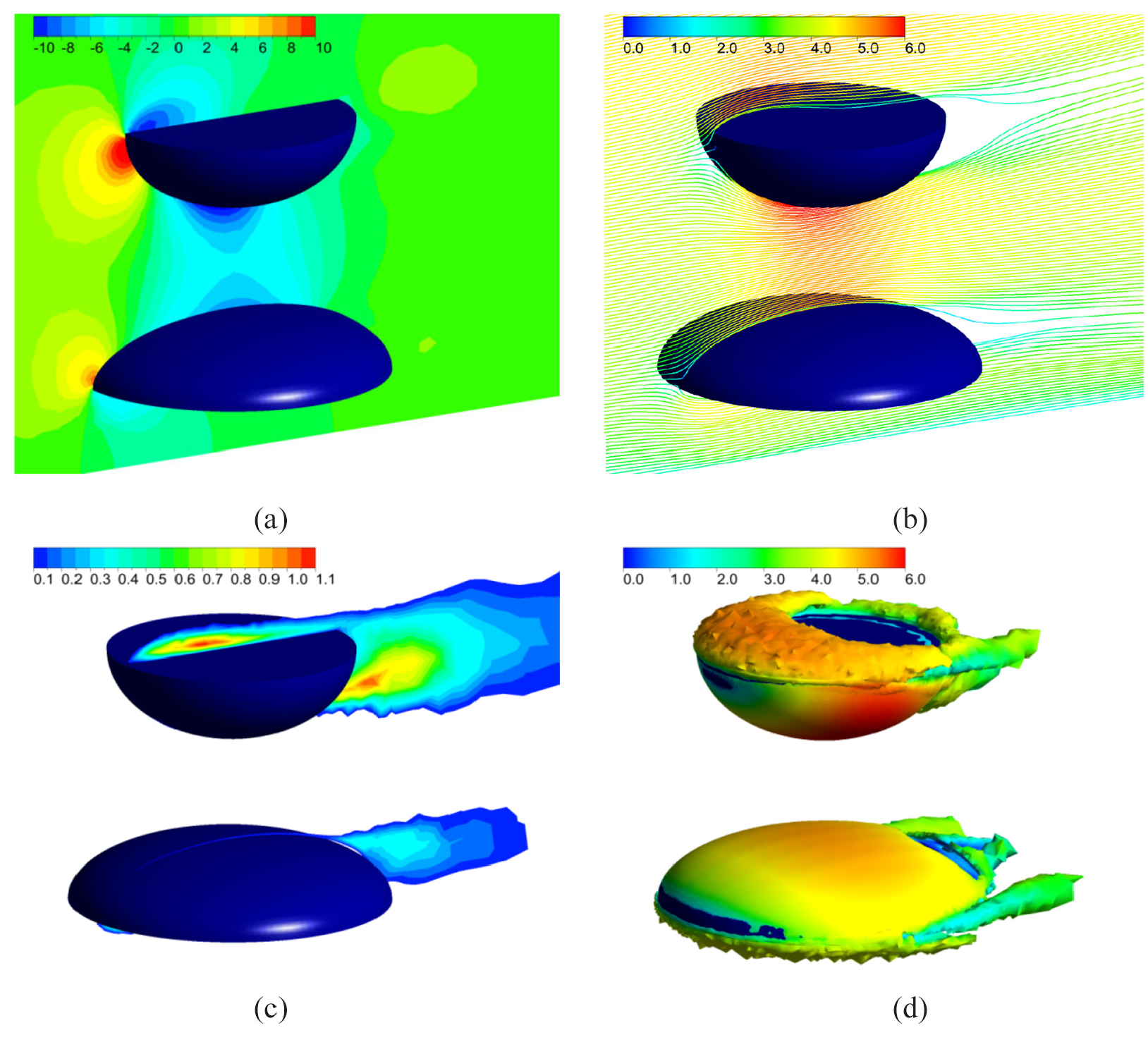
Computed: (a) gauge pressure in [Pa], (b) streamlines colored by velocity in [m/s], (c) turbulence kinetic energy in[m²/s²], and (d) vortex structures colored by velocity in [m/s].

Similar findings can be reached if contours of computed turbulence kinetic energy are considered (Figure 9(c)). The main sources of disturbances lie above the upper part and aft of the two halves of the flow concentrator, that is, in the zones that should not significantly affect the operation of the potential VAWT rotor. Flow slides smoothly along the flow concentrator, accelerating along the way, and only detaching after the planed VAWT rotor (and more massively from the upper, thicker half). Finally, Figure 9(d) illustrates the vortices that shed from the back sections of the two concentrator parts. Again, their intensity is not considerable and they should not pose a significant detriment to the VAWT aerodynamic performances.

The comparison of the velocity profiles (initial vs. improved) is illustrated in Figure 10. At first glance, it can be noted that the speed of approximately V_o = 4.12 m/s defined at the inlet (at the height of 2.75 m) can be accelerated to almost 5.0 m/s, that is, increased by nearly 22%. Furthermore, the velocity profile is visibly steadied and more evenly distributed which is particularly noticeable with the z-component that is nearly linear and symmetrical, Figure 10(b).

Figure 10.

Comparison of initial and computed velocity profiles in: (a) x-direction and (b) z-direction.

It is also worth mentioning that the differences in computed (by CFD) and predicted (by ANNs) output parameters of the chosen optimum are 0.75% for the average speed, and 2.33% for the min-to-max velocity ratio, which is quite satisfactory.

Effect of the wind turbine

Since the presence of a rotor significantly alters the initially straight flow by decelerating the axial and adding the rotational components to the wind velocity, it is also necessary to compare the performances of a chosen small-scale VAWT with and without the optimal flow concentrator, and thus truly justify the performed optimization study. Once again, the flow around a small-scale VAWT was computed using the numerical set-up previously described in section 2.1. The only difference is that, in this case, numerical mesh was even denser (containing over 2.1 million cells) since both the rotor blades and the flow concentrator were included. Figure 11 shows the two obtained power coefficient curves C_P(λ), while Figure 12 illustrates the instantaneous streamlines in the symmetry plane originating upstream from the VAWT rotor without and with the flow concentrator at optimal tip-speed ratios.

Figure 11.

Comparison of power coefficient curves of a small VAWT with and without the flow concentrator.

Figure 12.

Computed instantaneous streamlines around: (a) VAWT rotor and (b) VAWT rotor with flow concentrator colored by velocity in [m/s].

Somewhat lower performances of the smaller isolated rotor (C_P,_max ≈ 0.25) in comparison to the validation example (presented in Figure 2) can be explained by the viscosity effects that become more noticeable at lower Reynolds numbers as well as height dependent velocity profile (instead of uniform) defined along the inlet. Nonetheless, it can be noted that the usage of flow concentrator enables obtaining significantly higher values of maximal power coefficient, C_P,_max > 0.31, and consequently generated power. In the process, the power coefficient curve gets slightly elongated and translated to the right, implying that the optimal performance is now achieved at somewhat higher tip-speed ratios λ (i.e. smaller wind speeds V_o or higher angular velocities Ω). At the same time, the VAWT self-starting characteristics seem much improved and that power can now be generated at considerably lower values of tip-speed ratio λ (i.e. lower values of wind speed). Another benefit is that the area below the curve becomes enlarged resulting in a wider range of possible operating conditions.

By analyzing particular flow regimes (the optimal is depicted in Figure 12), it can be concluded that the rotational flow around VAWT rotor becomes steadied by the flow concentrator, all vortex shedding happens after the rotor, the overall deceleration of the free stream is more effective and that the expansion of streamlines aft of the rotor is increased. Also, a greater amount of air flows through the rotor thus enabling greater power extraction. Overall, the positive effects of the flow concentrator to wind turbine aerodynamic performances are undeniable, even at small scales and small velocities.

It should be mentioned that the VAWT rotor used in this section is a representative, rather than a final, optimal choice. VAWTs of different solidity and applied airfoil (even when the global characteristics remain the same) will perform quite differently when encompassed by a flow concentrator. Here, the geometry of the flow concentrator is primarily optimized for a particular location (where certain velocity profile should be expected). The combined pair of both optimal VAWT rotor and optimal flow concentrator will be the topic of future studies.

Conclusions

The most important lessons learned and gained experience by performing the described optimization procedures can be summed in several general and particular conclusions regarding the flow concentrator:

• – The addition of the unsymmetrical, specifically designed omnidirectional flow concentrator to a VAWT operating in Earth’s boundary layer can locally change the flow field in a favorable manner.

• – Expected increase of initially small axial wind velocity amounts to 20%–25% and produces a boost of generated mechanical power.

• – Relatively simple flow simulations of an isolated concentrator (instead of the complete system comprising both wind turbine rotor and flow concentrator) can be used for reliable estimations of possible velocity increase.

• – Half-ellipsoids of increased relative thickness produce more acceleration, but also earlier separation of the flow and higher drag.

• – Main contribution of the performed study is the coupled usage of novel computational, predictive and optimization tools and methods (CFD, ANN, and GA) in the discipline of renewable wind energy extraction.

• – Expected benefits of adding a flow concentrator to a VAWT rotor imply improved self-starting characteristics, increased maximal power coefficient, and expanded range of possible operating conditions at low manufacturing and maintenance costs.

• – Simple modifications and adjustments of the proposed methodology to other types of wind turbines, other choices of input and output parameters, different environmental conditions, etc. are also possible.