Sage Journals: Discover world-class research

Abstract

With regard to the structural characteristics of the McPherson suspension system, when a vehicle is being driven on a rough road surface, the force direction of the suspension varies. This poses challenges to the vehicle’s driving safety and handling stability. Based on Lagrangian equations, this paper proposes a new nonlinear semi-vehicle suspension model and presents comparative studies, conducted through simulation, on the estimated accuracy and computational overhead of the small-computational-overhead extended Kalman filter (EKF) and unscented Kalman estimation (UKF) methods, and on the effectiveness of the skyhook sliding mode control (SHSMC) and nonlinear skyhook-sliding mode control (NSHSMC) semi-active suspension control methods. The response of the vehicle to the state estimation algorithm was evaluated through computer simulations using the Carsim vehicle dynamic software. The simulation results reveal that the vehicle dynamic states were satisfactorily estimated when the vehicle was driven on a rough road surface. Compared with the small-computational-overhead EKF algorithm, the estimated results of these variables based on the UKF algorithm have higher accuracy. However, the UKF algorithm requires longer computation time compared with the EKF algorithm. The SHSMC control algorithm achieved greater improvement for the vehicle’s drive handling stability in the 6–10-Hz vibration region compared with the NSHSMC control algorithm. In a high-frequency region over 10Hz, the semi-active suspension controlled by the SHSMC method had a more adverse effect on the driving comfort.

Keywords

McPherson suspension Lagrangian equations state estimation NSHSMC controller

Introduction

Problem statement

Vehicle suspension is a device that controls the forces and moments induced by the road roughness on the wheels and acting on the vehicle body. Different suspension types have different mechanical mechanisms. McPherson’s independent suspension system is widely used as the front suspension of a vehicle. However, owing to this system’s structural characteristics, when the wheel moves up and down, the lateral swing of the wheel occurs, and the suspension system cannot resist the lateral impacts. The traditional vector linear model only considers the upward and downward movement of its sprung and un-sprung mass, and the lateral motion characteristics of the McPherson suspension cannot be effectively characterized.

When a vehicle is being driven on a rough road surface, the vehicle suspension system plays an important role in the vehicle’s ride comfort and handling stability. Notably, the ride comfort and handling stability are a pair of conflicting indices, that is, when the handling stability is improved, the ride comfort often deteriorates. Compared with passive suspension, semi-active suspension can be used to improve the handling stability without compromising the ride comfort.

Owing to the mechanical complexity of McPherson’s independent suspension system, it is necessary to accurately obtain the system’s mechanical dynamic states to realize the semi-active suspension control algorithm. With the least number of sensors, the states estimation algorithm can be used to estimate the mechanical signal, which is difficult to measure.

State of the art

Various studies have focused on vehicle dynamic models that include suspension mechanisms to investigate the dynamic performance of vehicles. Owing to the nonlinear geometrical effect of these mechanisms, the quarter-vehicle McPherson suspension nonlinear dynamic model has been investigated.^1–5 The above-mentioned studies are based on the dynamic model of a quarter-vehicle suspension system, assumed that the vehicle sprung mass only performs vertical motion, and ignored the roll motion of the vehicle sprung mass.

Based on the linear vector vehicle suspension model, the “skyhook damper” scheme, whereby a virtual damper is set between the vehicle sprung mass and the inertial reference, has been proposed.⁶ In recent years, based on the “skyhook damper” scheme, novel semi-active suspension control strategies and structures have been proposed.^7–10 Most modern vehicle control systems employ a feedback control structure. Therefore, the real-time estimation of the vehicle’s dynamic states is required to enhance the performance of the vehicle’s control system. Moreover, vehicle state estimation is becoming ever more relevant as chassis control systems are becoming increasingly sophisticated.¹¹ However, most existing studies on vehicle state estimation are based on the quarter traditional linear vector model, which is different to actual nonlinear suspension motion, and therefore results in estimation error. Furthermore, by comparing actual vehicles to the quarter-vehicle model used in the above-mentioned studies, it can be found that the system noise and measurement noise, which form owing to the wheel-road interaction on both sides of the vehicle, have an additive effect. Hence, the system noise and measurement noise variance must be re-determined.

In this study, by considering the mechanical structure characteristics of the McPherson suspension system, a semi-vehicle suspension dynamics model that considers the roughness of the road surface was established. Considering the superposition effect of the left and right road surface roughness excitation, the small-computational-overhead extended Kalman filter (EKF) and unscented Kalman estimation (UKF) state estimation algorithms of the semi-vehicle suspension dynamics model were developed. Additionally, the Semi-active suspension control algorithms, skyhook sliding mode control (SHSMC) and nonlinear skyhook sliding mode control (NSHSMC) were established. A road level classification algorithm based on the difference of dynamic states in the time and frequency domains has been proposed.^12,13 The road process noise variance matrices Q and measurement noise variance matrices R of the different levels of road roughness were provided to the above-mentioned Kalman filter algorithm. This study was structured as shown in Figure 1.

Figure 1.

Flow chart of Kalman estimation method for semi-vehicle semi-active suspension based on sliding mode control algorithm.

Contribution

(1) For the feasibility of implementation in onboard hardware, this paper discusses the estimated accuracy and computational overhead of the small-computational-overhead EKF and UKF state estimation methods for the vehicle suspension system when the vehicle is being driven on a rough road surface.

(2) To determine the advantages, disadvantages, and application field of the NSHSMC and SHSMC control algorithms, the vehicle’s drive handling stability and ride comfort with the semi-active suspension controlled by the NSHSMC and SHSMC control algorithms are discussed with regard to different frequency regions.

The rest of this paper is organized as follows. In Section 2, the wheel-road excitation model and a nonlinear semi-vehicle McPherson suspension model are established. In Section 3, the small-computational-overhead EKF and UKF algorithms are constructed, and the system noise and measurement noise variance are re-determined. In Section 4, the new nonlinear control algorithms of semi-active suspension, namely, NSHSMC and SHSMC, are proposed and their stability is verified. Finally, the conclusions drawn from this study are presented in Section 5.

Mathematical modeling

Road excitation

Road roughness function built using harmonic superposition method

As a source of system excitation, the road irregularities are analyzed using a typical ergodic stationary stochastic process.^14,15 The statistical characteristics of road irregularities are described by the power spectral density G_q (n). According to GB7031, the fitting expression of the road power spectral density is expressed as follows:

G_{q} (n) = G_{q} (n_{0}) {(\frac{n}{n_{0}})}^{- w} .

(1)

In equation (1), n₀ is the reference space frequency, and n₀ = 0.1 m⁻¹; G_q (n₀) is the road power spectral density under the reference space-frequency n₀; W is the frequency index, and W = 2.

The range of the spatial frequency n is (n₁, n₂).The road roughness variance is expressed as follows:

{σ_{z}}^{2} = \int_{n_{1}}^{n_{2}} G_{q} (n) dn .

(2)

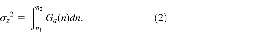
The interval (n₁, n₂) is divided into m small intervals. The power spectral density G_q (n_mid-i) at the center frequency n_mid-i (i = 1, 2, ···, m) of each interval replaces the spectral density values between the intervals. Equation (2) is approximately discretized as follows:

{σ_{z}}^{2} \approx \sum_{i = 1}^{m} G_{q} (n_{mid - i}) Δ n_{i .}

(3)

For each interval, the sinusoidal wave function with frequency n_mid-i (i = 1,2, ···, m) and standard deviation $\sqrt{G_{q} (n_{mid - i}) Δ n_{i}}$ is expressed as follows:

\sqrt{2 G_{q} (n_{mid - i}) Δ n_{i}} \sin (2 π n_{mid - i} I + θ_{i}) .

(4)

The sinusoidal wave function corresponding to each interval is superimposed to obtain the road surface roughness function model, as follows:

q (I) = \sum_{i = 1}^{m} \sqrt{2 G_{q} (n_{mid - i}) Δ n_{i}} \sin (2 π n_{mid - i} I + θ_{i}) .

(5)

In equation (5), I is the length of the road (m); Δn is the frequency interval (m⁻¹); θ_i is a random variable with [0, 2π] uniform distribution and independence. Then, equation (5), is converted to a time-domain model, as follows:

q (t) = \sum_{i = 1}^{m} \sqrt{2 G_{q} (n_{mid - i}) Δ n_{i}} \sin (2 π f_{mid - i} t + θ_{i}) .

(6)

In equation (6), t = I/u is time (s); f_mid-i = n_mid-iu is the time-frequency corresponding to n_mid-i (Hz), where u is the velocity of the vehicle (m/s).

Coherence of bilateral track excitation

The left and right road tracks have the same road roughness statistical characteristics and self-power spectral density on the same road. However, the random process of the road roughness of the two tracks has a cross-spectrum. The two tracks are coherent and the coherence strength is weak. In equation (6), θ_i is the key parameter of the coherence of the left and right track; therefore, θ_{i_right} can be obtained by fitting. The coherence exponentially decreases as follows^16,17:

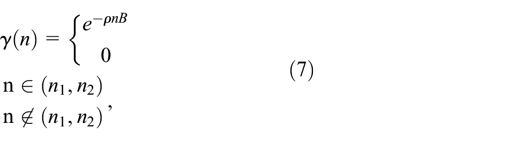
\begin{matrix} γ (n) = {\begin{matrix} e^{- ρ nB} \\ 0 \end{matrix} \\ \begin{matrix} n \in (n_{1}, n_{2}) \\ n \notin (n_{1}, n_{2}) \end{matrix}, \end{matrix}

(7)

Where ρ is an adjustment parameter and ρ = 1. Then, θ_{i_right} can be calculated as follows:

\begin{matrix} θ_{i_right} = \frac{e^{- 2 π B n^{1.5}}}{\sqrt{1 - e^{- 2 π B n^{1.5}}} + e^{- 2 π B n^{1.5}}} θ_{i_left} + \\ \frac{\sqrt{1 - e^{- 2 π B n^{1.5}}}}{\sqrt{1 - e^{- 2 π B n^{1.5}}} + e^{- 2 π B n^{1.5}}} θ_{i_new}, \end{matrix}

(8)

where θ_{i_new} is another new random number that is normally distributed on the [0, 2π] interval. Based on the above-mentioned analysis, let us consider that the vehicle speed is 80 km/h (22.2 m/s) and B is 1.4 m. A left and right road roughness time-domain model was established for an ISO road, and the model data were entered into Carsim to establish the Carsim road model.

New nonlinear semi-vehicle suspension model

In this study, a new nonlinear semi-vehicle suspension model was established for the Macpherson suspension system, as shown in Figure 2. The model includes a rigid chassis (1), control arm (6), wheel (5), damper (4), and coil spring (3) assemblies, and steering knuckle (2). The control arm is connected to the chassis with a rotational joint at point O and O′. The spherical joint connects the control arm at spindle B. The wheel is installed onto the steering knuckle. A cylindrical joint connects the steering knuckle to the damper, and the damper is connected to the chassis with a spherical joint at point A, as shown in Figure 2.

Figure 2.

New nonlinear semi-vehicle model.

Because the mass of the control arm is much smaller than the mass of the spring and un-spring mass, the mass of the control arm can be ignored. The entire system has four degrees of freedom. In this case, the generalized coordinates are the upward vertical displacement z_s, roll angle ϕ of the vehicle sprung mass, rotation angle of the right control arm θ_r counter-clockwise, and rotation angle of the left control arm θ_l clockwise.

The semi-vehicle suspension dynamic model is constructed based on the following assumptions:

(1) The un-sprung mass is linked to the chassis in two ways: through the damper and through the lower arm; θ_r and θ_l denote the angular displacement of the control arm.

(2) The sprung mass distribution coefficient ε of the front and rear axles of the vehicles is equal to one; that is, the front and rear half of the vehicle move independently in the vertical direction. The longitudinal effect of the road profile and the effect of the vehicle pitching motion are ignored.

(3) The bending and torsional deformation of the wheels and the effect of the wheel width are ignored.

Let z_ul and z_ur denote the vertical displacement of the center of mass of the left wheel C and right wheel C′, respectively, as follows:

z_{u r} = z_{s} + l_{0} φ \cos (r_{0} - φ) + l_{c} θ_{r},

(9a)

z_{u l} = z_{s} - l_{0} φ \cos (r_{0} + φ) + l_{c} θ_{l},

(9b)

where z_s is the vertical displacement of the vehicle body; O_m is the point of the vehicle roll center; O and O′ are the point of the mounting position of the rotational joint between the control arm and the vehicle chassis, respectively; r₀ is the initial angular displacement between O_mO and the horizontal direction; l₀ is the distance between O_m and O; l_c is the distance between O and C.

Here, θ₀ is the initial angular displacement of the control arm at the equilibrium state. Let α′ = α₀ + θ₀. α₀ be the initial angular displacement between the control arm and line OA or O′A′. Then, the following relationships can be obtained from triangle OAB and O′A′B′:

l_{r} = {(c_{r} - d_{r} \cos (α'))}^{\frac{1}{2}}, {l ’}_{r} = {(c_{r} - d_{r} \cos (α' - θ_{r}))}^{\frac{1}{2}},

(10a)

l_{l} = {(c_{r} - d_{r} \cos (α'))}^{\frac{1}{2}}, {l ’}_{l} = {(c_{r} - d_{r} \cos (α' - θ_{l}))}^{\frac{1}{2}},

(10b)

where l_r and l_l are the initial distance of A–B and A′–B′ at the equilibrium state, and l_r′ and l_l′ are the changes in the distance of A–B and A′–B′ with the rotation of the control arm by θ_r and θ_l; l_a is the distance between O and A, and l_a = OA; l_b is the distance between O and B, and l_b = OB.

c_{r} = l_{a}^{2} + l_{b}^{2}, d_{r} = 2 l_{a} l_{b}

(10c)

Then, the deflection of the spring can be expressed as follows:

Δ l_{l} = l'_{l} - l_{l}, Δ l_{r} = l'_{r} - l_{r},

(10d)

{\overset{\cdot}{l}}_{r} = 0, {\overset{\cdot}{l ’}}_{r} = \frac{d_{r} \sin (α_{0} + θ_{r}) {\overset{\cdot}{θ}}_{r}}{2 \sqrt{c_{r} - d_{r} \cos (α_{0} + θ_{r})}},

(10e)

{\overset{\cdot}{l}}_{l} = 0, {\overset{\cdot}{l ’}}_{l} = \frac{d_{r} \sin (α_{0} + θ_{l}) {\overset{\cdot}{θ}}_{l}}{2 \sqrt{c_{r} - d_{r} \cos (α_{0} + θ_{l})}},

(10f)

The relative velocity of the damper is expressed as follows:

Δ {\overset{\cdot}{l}}_{l} = \overset{\cdot}{l}'_{l} - {\overset{\cdot}{l}}_{l}, Δ {\overset{\cdot}{l}}_{r} = \overset{\cdot}{l}'_{r} - {\overset{\cdot}{l}}_{r} .

(10g)

Equations of motion

The motion equations of the new nonlinear semi-vehicle suspension model are derived using the second Lagrange equation. Among them, T, V, and D are the kinematic energy, potential energy, and damping function of the system, respectively.

T = \frac{1}{2} J {\overset{\cdot}{φ}}^{2} + \frac{1}{2} m_{c} {\overset{\cdot}{z}}_{s}^{2} + \frac{1}{2} m_{u} {({\overset{\cdot}{z}}_{ul} + {\overset{\cdot}{y}}_{ul})}^{2} + \frac{1}{2} m_{u} {({\overset{\cdot}{z}}_{ur} + {\overset{\cdot}{y}}_{ur})}^{2}

(11a)

\begin{matrix} V = \frac{1}{2} k_{s} {(Δ l_{l})}^{2} + \frac{1}{2} k_{s} {(Δ l_{r})}^{2} + \frac{1}{2} k_{t} {(z_{u l} - z_{l})}^{2} \\ + \frac{1}{2} k_{t} {(z_{u r} - z_{r})}^{2} \end{matrix}

(11b)

D = \frac{1}{2} c_{p} {(Δ {\overset{\cdot}{l}}_{l})}^{2} + \frac{1}{2} c_{p} {(Δ {\overset{\cdot}{l}}_{r})}^{2}

(11c)

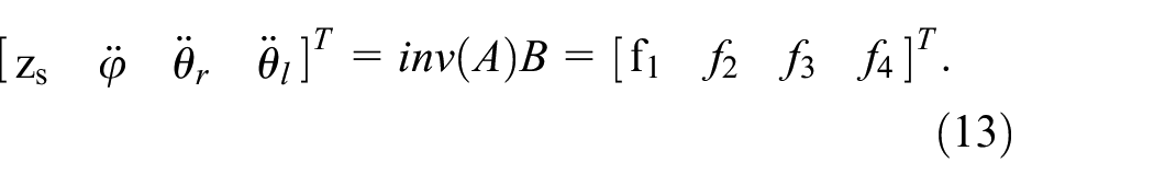
The state variables are introduced as q₁ = z_s, q₂ = ϕ, q₃ = θ_r, andq₄ = θ_l. Then, the dynamical model can be written in the state equation as follows:

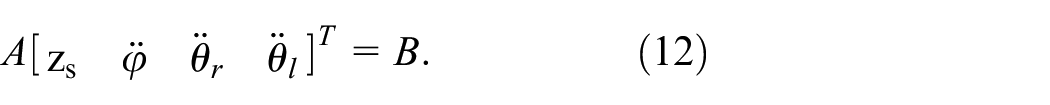
A {[\begin{matrix} {\overset{..}{z}}_{s} & \overset{..}{φ} & {\overset{..}{θ}}_{r} & {\overset{..}{θ}}_{l} \end{matrix}]}^{T} = B .

(12)

Then, equation (12) can be converted as follows:

{[\begin{matrix} {\overset{..}{z}}_{s} & \overset{..}{φ} & {\overset{..}{θ}}_{r} & {\overset{..}{θ}}_{l} \end{matrix}]}^{T} = i n v (A) B = {[\begin{matrix} f_{1} & f_{2} & f_{3} & f_{4} \end{matrix}]}^{T} .

(13)

It is assumed that the vehicle system state vector is selected as follows:

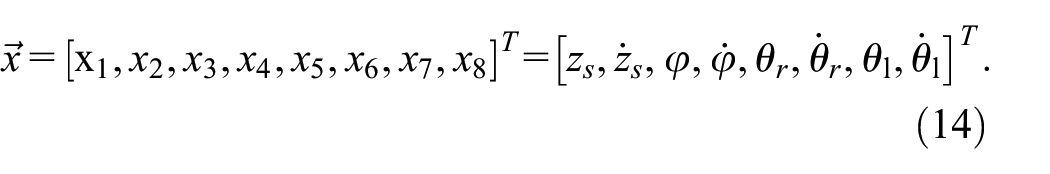
\vec{x} = {[x_{1}, x_{2}, x_{3}, x_{4}, x_{5}, x_{6}, x_{7}, x_{8}]}^{T} = {[z_{s}, {\overset{\cdot}{z}}_{s}, φ, \overset{\cdot}{φ}, θ_{r}, {\overset{\cdot}{θ}}_{r}, θ_{l}, {\overset{\cdot}{θ}}_{l}]}^{T} .

(14)

Then, the motion equations of the new nonlinear semi-vehicle suspension model can be written as follows.

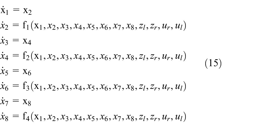
\begin{matrix} {\overset{\cdot}{x}}_{1} = x_{2} \\ {\overset{\cdot}{x}}_{2} = f_{1} (x_{1}, x_{2}, x_{3}, x_{4}, x_{5}, x_{6}, x_{7}, x_{8}, z_{l}, z_{r}, u_{r}, u_{l}) \\ {\overset{\cdot}{x}}_{3} = x_{4} \\ {\overset{\cdot}{x}}_{4} = f_{2} (x_{1}, x_{2}, x_{3}, x_{4}, x_{5}, x_{6}, x_{7}, x_{8}, z_{l}, z_{r}, u_{r}, u_{l}) \\ {\overset{\cdot}{x}}_{5} = x_{6} \\ {\overset{\cdot}{x}}_{6} = f_{3} (x_{1}, x_{2}, x_{3}, x_{4}, x_{5}, x_{6}, x_{7}, x_{8}, z_{l}, z_{r}, u_{r}, u_{l}) \\ {\overset{\cdot}{x}}_{7} = x_{8} \\ {\overset{\cdot}{x}}_{8} = f_{4} (x_{1}, x_{2}, x_{3}, x_{4}, x_{5}, x_{6}, x_{7}, x_{8}, z_{l}, z_{r}, u_{r}, u_{l}) \end{matrix}

(15)

The nonlinear system equation (15) can be written in vector form, as follows:

\vec{\overset{\cdot}{x}} = f (x_{1}, x_{2}, x_{3}, x_{4}, x_{5}, x_{6}, x_{7}, x_{8}, z_{l}, z_{r}, u_{r}, u_{l}) .

(16)

Vehicle dynamic state estimator

Small-computational-overhead EKF method

Regarding the nonlinear discrete-time system expressed in equation (16), for the EKF, in each sampling time, the state transition matrix of the system is replaced by the Jacobian matrix of f at the k-step prediction value. Compared with the linear Kalman estimation method, the computational overhead is much larger. In this study, the system state variables fluctuated around the equilibrium state (x_1e, x_2e, x_3e, x_4e, x_5e, x_6e, x_7e, x_8e) = (0, 0, 0, 0, 0, 0, 0, 0). The small-computational-overhead EKF method is proposed to reduce the computational overhead.

The highly nonlinear equations of the semi-vehicle suspension model are linearized at the equilibrium state, as follows:

\overset{\cdot}{\vec{x}} = C \cdot \vec{x} + E_{1} \cdot u_{l} + E_{2} \cdot u_{r} + D_{1} \cdot z_{l} + D_{2} \cdot z_{r},

(17)

\vec{y} = H \cdot \vec{x},

(18)

where C, E₁, E₂, D₁, D₂, and H are as described in the appendix.

To investigate the observability and controllability of the systems expressed in equations (17) and (18), the following transformation was considered:

u' = [u_{l}; u_{r}; z_{l}; z_{r}], b = [E_{1}, E_{2}, D_{1}, D_{2}] .

Equations (17) and (18) are converted to:

\overset{\cdot}{\vec{x}} = C \cdot \vec{x} + b \cdot u',

(19)

\vec{y} = H \cdot \vec{x},

(20)

where

\begin{matrix} M = [\begin{matrix} b & Cb & C^{2} b \dots C^{n - 1} b \end{matrix}], rank (M) = 8, \end{matrix}

\begin{matrix} N = [\begin{matrix} H \\ HC \\ ⋮ \\ H C^{n - 1} \end{matrix}], rank (N) = 8 . \end{matrix}

Hence, the system is completely observable and controllable.

When a vehicle is being driven on a rough road surface, to use the Kalman filter algorithm and estimate the vehicle dynamic state based on (2.2), equation (19) is discretized as follows:

\begin{matrix} {\vec{x}}_{k + 1} = {\vec{x}}_{k} + Δ t \cdot {\overset{\cdot}{\vec{x}}}_{k} \\ = {\vec{x}}_{k} + Δ t \cdot (C \cdot {\vec{x}}_{k} + E_{1} \cdot u_{lk} + E_{2} \cdot u_{rk} \\ + D_{1} \cdot x_{lk} + D_{2} \cdot x_{rk}), \\ = Φ \cdot {\vec{x}}_{k} + B \cdot {\vec{u}}_{k} + Γ \cdot {\vec{w}}_{k} \end{matrix}

(21)

{\vec{y}}_{k + 1} = H \cdot {\vec{x}}_{k + 1} + {\vec{v}}_{k + 1} .

(22)

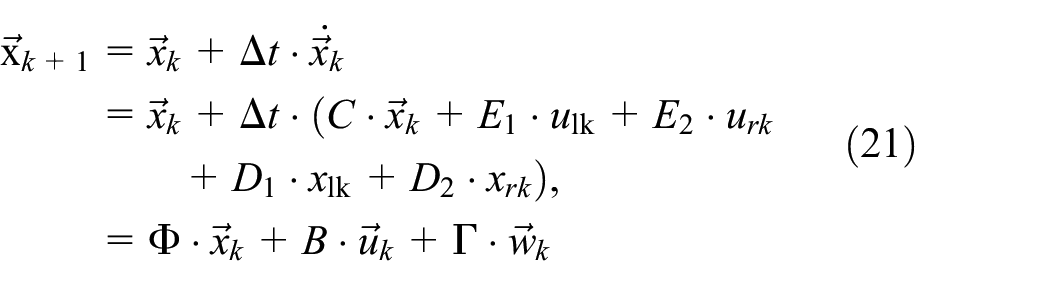
Here, Δt is the time step, k represents the state at sampling time Δt·k. In equations (21) and (22), is an 8 × 1 state vector; Φ is an 8 × 8 system transi is a 2 × 1 control input matrix; Γ is an 8 × 2 constant input matrix; ${\vec{w}}_{k}$ (2 × 1)and ${\vec{v}}_{k + 1}$ (3 × 1) represent uncorrelated Gaussian white noise sequences.

The 3 × 1 measured signal vector at time k+1 is ${\vec{y}}_{k + 1} = {[y_{1, k + 1}, y_{2, k + 1}, y_{3, k + 1}]}^{T} = {[{\overset{\cdot}{z}}_{s, k + 1}, θ_{r, k + 1}, θ_{l, k + 1}]}^{T}$ , where ${\overset{\cdot}{z}}_{s, k + 1}$ is the spring-mass vertical velocity signal; $θ_{l, k + 1}$ and $θ_{r, k + 1}$ are the left and right control arm swing angular displacement signal, respectively.

Based on the above analysis, by combining the discrete-time state equations (21) and (22) for each state, the Kalman filter algorithm is reduced to the following expressions:

{\hat{x}}_{(0 | 0)} = μ_{0}; p_{(0 | 0)} = p_{0},

(23)

{\hat{x}}_{(k + 1 | k)} = Φ {\hat{x}}_{(k | k)} + B \cdot {\bar{u}}_{k},

(24)

1006188,

(25)

K_{(k + 1)} = P_{(k + 1 | k)} H^{T} {[H P_{(k + 1 | k)} H^{T} + R]}^{- 1},

(26)

ε_{(k + 1)} = Y_{(k + 1)} - H {\hat{x}}_{(k + 1 | k)},

(27)

P_{(k + 1 | k + 1)} = [I_{n} - K_{(k + 1)} H] P_{(k + 1 | k)},

(28)

{\hat{x}}_{(k + 1 | k + 1)} = {\hat{x}}_{(k + 1 | k)} + K_{(k + 1)} ε_{(k + 1)} .

(29)

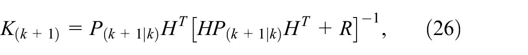
Equation (24) describes the prediction process from the estimated state at time k to the state at time k + 1. Equation (25) quantitatively describes the prediction process, where P_(k/k) is the estimation error variance matrix, K_(k+1) is the Kalman gain, μ₀ is the system initial state, and P₀ is the initial estimation error variance matrix.

Unscented Kalman estimation method

In Julier and Uhlmann,¹⁹ the unscented Kalman estimation method (UKF) was proposed for nonlinear systems. The nonlinear system equation (16) is converted to a nonlinear discrete-time state equation, as follows:

{\vec{x}}_{k + 1} = F ({\vec{x}}_{k}, u_{r, k}, u_{l, k}) .

(30)

The measurement equation is expressed as follows:

{\vec{y}}_{k + 1} = H \cdot {\vec{x}}_{k + 1} .

(31)

The UKF is expressed as follows:

Initialize with:

\begin{matrix} {\hat{x}}_{(0 | 0)} = E (x_{0}) \\ P_{(0 | 0)} = E [(x_{0} - {\hat{x}}_{(0 | 0)}) {(x_{0} - {\hat{x}}_{(0 | 0)})}^{T}] . \end{matrix}

(32)

Calculate the sigma points:

χ^{(i)} (k | k) = [\begin{matrix} {\hat{x}}_{(k | k)} & {\hat{x}}_{(k | k)} + \sqrt{(n + λ) P_{(k | k)}} & {\hat{x}}_{(k | k)} - \sqrt{(n + λ) P_{(k | k)}} \end{matrix}],

(33)

\begin{matrix} ω_{m}^{0} = \frac{λ}{λ + n} \\ ω_{c}^{0} = \frac{λ}{λ + n} + 1 - α^{2} + β, \end{matrix}

(34)

ω_{c}^{i} = ω_{m}^{i} = \frac{1}{2} (λ + n) i = 1, 2 \dots n,

(35)

where $λ = α^{2} (L + κ) - L$ is a scaling parameter; α is set to 1e-3, κ is set to zero, and β is set to 2.The relevant details are provided in Wan and Merwe.²⁰

Time update:

χ^{(i)} (k + 1 | k) = F (χ^{(i)} (k | k), u_{r, k}, u_{l, k}),

(36)

Y^{(i)} (k + 1 | k) = H \cdot χ^{(i)} (k + 1 | k),

(37)

\hat{x} (k + 1 | k) = \sum_{i = 1}^{2 n} ω^{(i)} χ^{(i)} (k + 1 | k) .

(38)

Measurement update:

\begin{matrix} P (k + 1 | k) = \sum_{i = 1}^{2 n} ω^{(i)} [\hat{x} (k + 1 | k) - χ^{(i)} (k + 1 | k)] \\ {[\hat{x} (k + 1 | k) - χ^{(i)} (k + 1 | k)]}^{T} + Q, \end{matrix}

(39)

\bar{Y} (k + 1 | k) = \sum_{i = 1}^{2 n} ω^{(i)} Y^{(i)} (k + 1 | k),

(40)

\begin{matrix} P_{y_{k} y_{k}} = \sum_{i = 0}^{2 n} ω^{(i)} [Y^{(i)} (k + 1 | k) - \bar{Y} (k + 1 | k)] \\ {[Y^{(i)} (k + 1 | k) - \bar{Y} (k + 1 | k)]}^{T} + R, \end{matrix}

(41)

\begin{matrix} P_{x_{k} y_{k}} = \sum_{i = 0}^{2 n} ω^{(i)} [χ^{(i)} (k + 1 | k) - \bar{Y} (k + 1 | k)] \\ {[χ^{(i)} (k + 1 | k) - \bar{Y} (k + 1 | k)]}^{T}, \end{matrix}

(42)

K (k + 1) = P_{x_{k} y_{k}} P_{y_{k} y_{k}}^{- 1},

(43)

\begin{matrix} \hat{x} (k + 1 | k + 1) = \hat{x} (k + 1 | k) + K (k + 1) \\ [{\vec{y}}_{k + 1} - \bar{Y} (k + 1 | k)], \end{matrix}

(44)

P (k + 1 | k + 1) = P (k + 1 | k) - K (k + 1) P_{y_{k} y_{k}} K^{T} (k + 1) .

(45)

Estimation of road process noise variance matrices Q and measurement noise variance matrices R

In equations (25), (26), (39), and (41), the tuning operation of Q and R is a critical step for the accuracy of the estimation and control algorithm. These two parameters should be defined using a priori knowledge about the perturbation ${\vec{w}}_{k}$ acting on the nonlinear system equation, and ${\vec{v}}_{k + 1}$ acting on the measurement equation; Q and R are the corresponding process noise variance and measurement noise variance matrices, respectively. Notably, Q and R are bounded positive definite matrices (that is Q > 0, R > 0).

To obtain an optimal solution with the Kalman filter, it is assumed that the roughness of the road profile is Gaussian white noise. The noise ${\vec{w}}_{k}$ is Gaussian white noise. Using the road excitation model proposed in Sections 2.1, the system process noise variance Q under different road excitation levels can easily be obtained, and the upper and lower spatial frequencies n₂ and n₁ are set as 2.83 m⁻¹ and 0.011 m⁻¹.

Q_{q} = {σ_{q}}^{2} = \int_{n_{1}}^{n_{2}} G_{q} (n) dn

(46)

Based on the above analysis, the Q_q = E(w_kw_k^T) of the state estimator under different road levels(A-H) of the quarter vehicle are listed in Table 1.

Table 1.

System process noise variance Q_q from single wheel-road surface interaction.

Road level	Q_q (10⁻⁶ m²)(0.011 m⁻¹ < n < 2.83 m⁻¹)	Road level	Q_q (10⁻⁶ m²)(0.011 m⁻¹ <n < 2.83 m⁻¹)
A	14.52	E	3708.81
B	57.91	F	14835.24
C	231.95	G	59345.83
D	927.2	H	237383.33

The semi-vehicle model established in this study was compared to the quarter-vehicle model. While the vehicle is being driven, the wheels on both sides of the vehicle interact with the road at the same time, and there are multiple process noise w_k and measurement noise v_k+1 sources of input to the vehicle during the driving process, owing to the superposition effect.

Let us assume that the distribution of the road surface roughness in all directions is isotropic Gaussian distribution. Then, the correlation function between two values of road surface roughness is a function only of the distance between them.

R_{q} (B) = \int_{n_{1}}^{n_{2}} G_{q} (n) \cdot e^{i 2 π n B} d n,

(47)

Let us assume that $R_{q} (B)$ is constant under a certain level of road surface roughness.

C o v (w_{kl}, w_{kr}) = R_{q} (B) \cdot \sqrt{Q_{q}} \cdot \sqrt{Q_{q}},

(48)

The estimation algorithm processes noise variance Q, as follows:

\begin{matrix} q_{i} = Γ^{2} (i, 1) \cdot D (w_{kl}) + Γ^{2} (i, 2) \cdot D (w_{kr}) \\ + 2 \cdot Γ (i, 1) \cdot Γ (i, 2) \cdot Cov (w_{kl}, w_{kr}) \\ = (Γ^{2} (i, 1) + Γ^{2} (i, 2)) \cdot Q_{q} + 2 \cdot Γ (i, 1) \cdot Γ (i, 2) \\ \cdot Cov (w_{kl}, w_{kr}), \end{matrix}

(49)

Q = diag [\begin{matrix} q_{1}, & q_{2}, & q_{3}, & q_{4}, & q_{5}, & q_{6}, & q_{7}, & q_{8} \end{matrix}] .

(50)

Many previous studies assumed that the value of R is constant and can be determined through empirical assessments for Kalman filter applications. However, the test equipment operates in a vibration environment with a rough road surface and the above-mentioned superimposed effects. The statistical characteristics of the measurement noise v_k are affected and change, which increases the deviation between the estimated value and the actual value, and results in the divergence of the estimation algorithm. The method used to determine R in this study is described below.¹⁸

In the measurement equation, the actual values of ${\vec{v}}_{k + 1}$ are unknown. Let us assume that $E (\vec{v}) = \vec{r}$ and $E (\vec{v} {\vec{v}}^{T}) = R$ . The measurement innovation is defined as follows:

{\vec{r}}_{k + 1} = {\vec{y}}_{k + 1} - H \cdot {\vec{x}}_{k + 1 | k} .

(51)

Let us assume that ${{\vec{r}}_{k}}$ is a zero-mean white noise sequence, whose variance is expressed as follows:

E ({\vec{r}}_{k + 1} {\vec{r}}_{j + 1}^{T}) = {\begin{matrix} 0 & (k \neq j) \\ R_{k + 1} + H P_{k + 1} H^{T} & (k = j) \end{matrix},

(52)

Where $R_{k + 1}$ is the variance matrix for the measured noise, and $P_{k + 1}$ is the estimation error variance matrix in the estimation method.

Let us assume that ${\vec{v}}_{k}$ (k = 1, 2, ···N) in the measurement equation are not correlated, and $\vec{r}$ and R are constant. Then, the sampling value of the measured noise ${\vec{r}}_{k}$ (k = 1, 2, ···N)is an element of Ω_R = { ${\vec{v}}_{k}$ }. Based on the noise sampling ${\vec{r}}_{k}$ obtained in Ω_R, the unbiased estimation of $\vec{r}$ can be carried out as follows:

\hat{\vec{r}} = \frac{1}{N} \sum_{k = 1}^{N} {\vec{r}}_{k} .

(53)

The unbiased estimation of C_r can be carried out as follows:

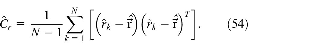
{\hat{C}}_{r} = \frac{1}{N - 1} \sum_{k = 1}^{N} [({\hat{r}}_{k} - \hat{\vec{r}}) {({\hat{r}}_{k} - \hat{\vec{r}})}^{T}] .

(54)

The expectation of ${\hat{C}}_{r}$ is expressed as follows:

E ({\hat{C}}_{r}) = \frac{1}{N} \sum_{k = 1}^{N} H P_{k + 1 | k} H^{T} + R_{k + 1} .

(55)

The estimation algorithm processes noise variance $R_{k + 1}$ of the test equipment as follows:

\begin{matrix} R_{k + 1} = \frac{1}{N - 1} \sum_{k = 1}^{N} \\ [({\hat{r}}_{k} - \hat{\vec{r}}) {({\hat{r}}_{k} - \hat{\vec{r}})}^{T} - \frac{N - 1}{N} H P_{k + 1 | k} H^{T}] . \end{matrix}

(56)

In Qin et al.,¹² a road classification algorithm is proposed to classify the road roughness levels based on the time and frequency domain signals for different road roughness levels. In this study, this method was used to classify the uneven levels of the road online. When the vehicle is driven on different road levels, it provides real-time Q and R values to the estimator.

The parameters considered in the investigation of the dynamic state estimation algorithm and control algorithm of the semi-active suspension system are listed in Table 2.

Table 2.

Model parameters.

Mechanical parameters			Geometric parameters
J (kg·m²)	Inertia moment ofvehicle roll motion	1220	l₀ (m)	0.5
m_c (kg)	Sprung mass	1800/2	l_a (m)	0.5
m_u (kg)	Un-sprung mass	70	l_b (m)	0.5
c_p (N·s/m)	Suspension damping	2050	l_c (m)	0.6
k_s (N/m)	Suspension stiffness	17658	a₀ (°)	45
k_t (N/m)	Tyre vertical stiffness	183887	r₀ (°)	35

State estimation results

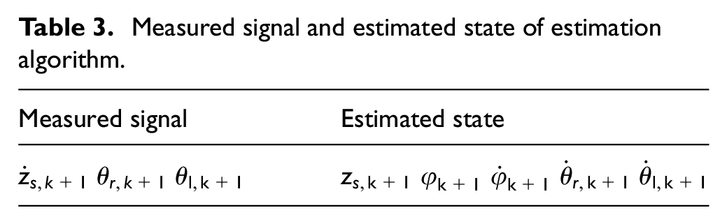
The effectiveness of the extended and unscented Kalman estimation methods proposed in Section 3.1 for a vehicle being driven on different road levels was verified. The system definition in Table 2 was adopted, and the vehicle velocity was set to 80 km/h (22.2 m/s). Based on the vehicle model constructed in Section 2.2, the vehicle was driven on ISO Level-B, -D, and -F roads. As presented in Table 3, the 3 × 1 measured signal vector [ ${\overset{\cdot}{z}}_{s, k + 1}$ ; $θ_{lk}$ ; $θ_{rk}$ ] of the vehicle to the state estimation algorithm was evaluated using the vehicle dynamics software Carsim. The estimated results of the vehicle dynamic states, which were obtained while the vehicle was being driven on constructed roads, are presented in Figure 3.

Table 3.

Measured signal and estimated state of estimation algorithm.

Measured signal	Estimated state
${\overset{\cdot}{z}}_{s, k + 1}$ $θ_{r, k + 1}$ $θ_{l, k + 1}$	$z_{s, k + 1}$ $φ_{k + 1}$ ${\overset{\cdot}{φ}}_{k + 1}$ ${\overset{\cdot}{θ}}_{r, k + 1}$ ${\overset{\cdot}{θ}}_{l, k + 1}$

Figure 3.

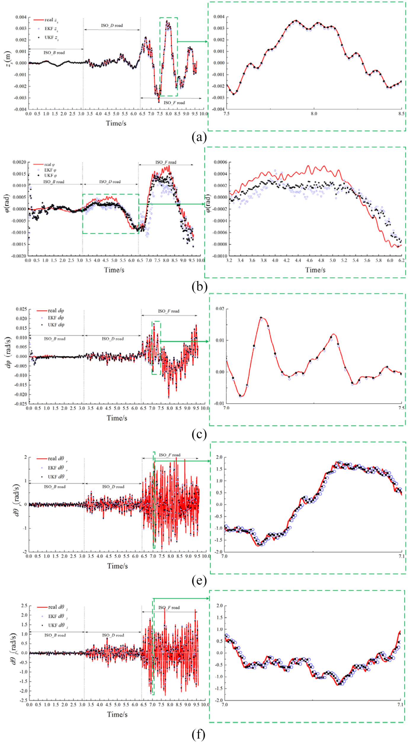
Estimation results for dynamic states of vehicle driven on ISO-B,-D, and -F road surfaces: (a) $z_{s}$ , (b) $φ$ , (c) $\overset{\cdot}{φ}$ , (d) ${\overset{\cdot}{θ}}_{r}$ , and (e) ${\overset{\cdot}{θ}}_{l}$ .

Based on the small-computational-overhead EKF and UKF methods, as shown in Figure 3, when the vehicle was driven on ISO Level-B, -D, and -F rough road surfaces, the actual dynamic state variables of the vehicle and the estimated results of these variables exhibited the same change pattern. The above-mentioned vehicle dynamic states (a) $z_{s}$ , (b) $φ$ , (c) $\overset{\cdot}{φ}$ , (d) ${\overset{\cdot}{θ}}_{r}$ , and (e) ${\overset{\cdot}{θ}}_{l}$ were satisfactorily estimated when the vehicle was driven on a rough road surface. Compared with the small-computational-overhead EKF algorithm, the estimation results for these variables based on the UKF algorithm were more accurate. However, the UKF algorithm required longer computation time for each step compared with the small-computational-overhead EKF algorithm.

For the proposed estimation method, the sampling time was set to 0.001 s, and the computation times of the small-computational-overhead EKF and UKF are shown in Figure 4.

Figure 4.

Computation time of small-computational-overhead EKF and UKF.

Nonlinear reference mode sliding mode control algorithm

Karnopp proposed the “skyhook damper” scheme of passive suspension as a reference model to achieve the minimum $c_{1} E ({\overset{\cdot}{x}}_{br}^{2}) + c_{2} E {(x_{br} - x_{w})}^{2}$ , where x_br and x_w are the vertical displacements of the reference model sprung mass and un-sprung mass, respectively; E ( ) denotes the “expected value.” However, it is not possible to connect a damper from the isolated mass to an inertial reference. In this study, the control objective was to force the semi-active suspension system of the semi-vehicle to behave as the “skyhook damper” reference model by introducing an appropriate control input. The difference between the response provided by the reference model and the actual system was calculated using the sliding mode control (SMC) strategy.

Skyhook sliding mode control algorithm (SHSMC)

For a nonlinear semi-vehicle model, a semi-active suspension control algorithm is proposed by combining the “skyhook” reference mode and SMC strategy algorithms, based on the above Kalman state estimation method. The dynamical equation of the quarter vehicle sprung mass is expressed as follows:

m_{b} {\overset{\cdot\cdot}{x}}_{b} + k_{s} (x_{b} - x_{w}) + c_{p} ({\overset{\cdot}{x}}_{b} - {\overset{\cdot}{x}}_{w}) - u = 0 .

(57)

Equation (57) can be expressed in the form of a state equation, as follows:

[\begin{matrix} {\overset{\cdot}{x}}_{b} \\ {\overset{\cdot\cdot}{x}}_{b} \end{matrix}] = [\begin{matrix} 0 & 1 \\ - \frac{k_{s}}{m_{b}} & - \frac{c_{p}}{m_{b}} \end{matrix}] [\begin{matrix} x_{b} \\ {\overset{\cdot}{x}}_{b} \end{matrix}] + [\begin{matrix} 0 & 0 \\ \frac{k_{s}}{m_{b}} & \frac{c_{p}}{m_{b}} \end{matrix}] [\begin{matrix} x_{w} \\ {\overset{\cdot}{x}}_{w} \end{matrix}] + [\begin{matrix} 0 \\ \frac{1}{m_{b}} \end{matrix}] u,

where m_b is the sprung mass of the quarter vehicle model, x_b and x_w are the vertical displacement of the sprung mass and un-sprung mass, k_s and c_p are the suspension stiffness and damping coefficient, u is the semi-active suspension control force acting on the vehicle. In actual applications, it is impossible to realize the synchronous excitation of the reference model and actual model on the actual road surface. During the simulation, the reference Skyhook model is expressed as follows:

m_{b} {\overset{\cdot\cdot}{x}}_{br} + k_{s} (x_{br} - x_{w}) + c_{sky - hook} {\overset{\cdot}{x}}_{br} = 0 .

(58)

Equation (58) can be expressed in the form of a state equation, as follows:

[\begin{matrix} {\overset{\cdot}{x}}_{br} \\ {\overset{\cdot\cdot}{x}}_{br} \end{matrix}] = [\begin{matrix} 0 & 1 \\ - \frac{k_{s}}{m_{b}} & - \frac{c_{sky - hook}}{m_{b}} \end{matrix}] [\begin{matrix} x_{br} \\ {\overset{\cdot}{x}}_{br} \end{matrix}] + [\begin{matrix} 0 & 0 \\ \frac{k_{s}}{m_{b}} & 0 \end{matrix}] [\begin{matrix} x_{w} \\ {\overset{\cdot}{x}}_{w} \end{matrix}],

where c_sky-hook is the damping coefficient between the reference model sprung mass and the inertial reference. The system tracking error is defined as follows:

\tilde{x} = {[\begin{matrix} \int (x_{b} - x_{br}) dt & x_{b} - x_{br} & {\overset{\cdot}{x}}_{b} - {\overset{\cdot}{x}}_{br} \end{matrix}]}^{T} .

(59)

The system tracking error equation (59) can be rewritten in a state-space form, as follows:

\overset{\cdot}{\tilde{x}} = A_{\tilde{x}} \tilde{x} + K_{\tilde{x}} {\overset{\cdot}{x}}_{w} + B_{\tilde{x}} u,

(60)

where:

\begin{matrix} A_{\tilde{x}} = [\begin{matrix} 0 & 1 & 0 \\ 0 & 0 & 1 \\ 0 & - k_{s} / m_{b} & - c_{sky - hook} / m_{b} \end{matrix}], \\ K_{\tilde{x}} = [\begin{matrix} 0 \\ 0 \\ c_{sky - hook} / m_{b} \end{matrix}], B_{\tilde{x}} = [\begin{matrix} 0 \\ 0 \\ 1 / m_{b} \end{matrix}] . \end{matrix}

The system switching surface is defined as follows:

σ = ({\overset{\cdot}{x}}_{b} - {\overset{\cdot}{x}}_{br}) + c_{1} (x_{b} - x_{br}) + c_{0} \int (x_{b} - x_{br}) dt,

(61)

where c₁ and c₀ satisfy Hurwitz’s conditions. Equation (61) is differentiated once, as follows:

\overset{\cdot}{σ} = ({\overset{\cdot\cdot}{x}}_{b} - {\overset{\cdot\cdot}{x}}_{br}) + c_{1} ({\overset{\cdot}{x}}_{b} - {\overset{\cdot}{x}}_{br}) + c_{0} (x_{b} - x_{br}) .

(62)

To force the system dynamics to reach the sliding surface, the following system reaching law is used:

\overset{\cdot}{σ} = - ε_{1} sgn (σ) - ε_{2} σ .

(63)

To weaken the system chatter, when s is sufficiently small, the following relationships are used:

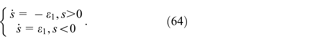
{\begin{matrix} \overset{\cdot}{s} = - ε_{1}, s > 0 \\ \overset{\cdot}{s} = ε_{1}, s < 0 \end{matrix} .

(64)

At this time, ε₁ is the movement speed gain when the states reach the sliding mode surface σ. When the states pass through the sliding mode surface, a small ε₁ can ensure that the approach speed is relatively small, and thereby small system chatter is ensured. However, because the system reaching law $\overset{\cdot}{σ}$ consists of ε₁ and ε₂, if ε₁ is simply reduced, the overall approach speed outside the sliding mode surface will also be reduced. Therefore, when ε₁ is reduced, ε₂ should be appropriately increased to ensure the system’s overall approach speed. In this study, ε₁ = 1 and ε₂ = 15 were selected. Then, the control force of the semi-active suspension controlled by the SHSMC can be expressed as follows:

\begin{matrix} u = (c_{sky - hook} - c_{1} m_{b}) ({\overset{\cdot}{x}}_{b} - {\overset{\cdot}{x}}_{br}) + (k_{s} - c_{0} m_{b}) (x_{b} - x_{br}) . \\ - c_{sky - hook} {\overset{\cdot}{x}}_{w} - ε_{1} m_{b} sgn (σ) - ε_{2} m_{b} σ \end{matrix}

(65)

The control force of the semi-active suspension controlled by the SHSMC control algorithm was used as input to the vehicle dynamics software Carsim. According to the vehicle’s structural geometry presented in Table 2, the SHSMC control algorithm’s signal input $x_{b}^{l}$ and $x_{wl}$ on the left side, and $x_{b}^{r}$ and $x_{wr}$ on the right side, can be calculated as follows:

x_{b}^{l} = z_{s} - l_{a} \hat{φ},

(66)

x_{wl} = z_{s} - l_{o} \hat{φ} + l_{c} θ_{l},

(67)

x_{b}^{r} = z_{s} + l_{a} \hat{φ},

(68)

x_{wr} = z_{s} + l_{o} \hat{φ} + l_{c} θ_{r},

(69)

where $x_{b}$ in equation (57) corresponds to $x_{b}^{l}$ in equation (66) and $x_{b}^{r}$ in equation (68) of the semi-active suspension systems; $x_{w}$ corresponds to $x_{wl}$ in equation (67) and $x_{wr}$ in equation (69) of the semi-active suspension systems; $\hat{φ}$ is the roll angular of the sprung mass. The Kalman state estimation method is used to estimate the dynamic state parameters of the vehicle for the control algorithm.

New nonlinear Skyhook-SMC control algorithm

This section proposes the new NSHSMC control algorithm, whose control structure is shown in Figure 5. According to the mechanical structural characteristics of the Macpherson suspension system, new quarter reference models and new quarter decomposition models of the nonlinear Macpherson suspension system are established on the left and right sides of the vehicle. As shown in Figure 5, there are four sub-models in total. In the process of constructing the above-mentioned sub-models, the following assumptions were made.

(1) The horizontal movement of the sprung mass is ignored, that is, the sprung mass only had vertical displacement z_s.

(2) The sprung mass of the quarter vehicle is 1/4 of the vehicle sprung mass, $m_{bc} = m_{c} / m_{c} 4 4$ .

(3) The mass and stiffness of the control arm are ignored.

(4) The coil spring deflection, wheel deflection, and damping forces are in the linear regions of their operating ranges.

(5) For the left decomposition model, the vertical displacement of the sprung mass is expressed as follows:

z'_{cl} = z_{s} - l_{0} \hat{φ} .

(70)

The vertical displacement of the un-sprung mass is expressed as follows:

z_{ul} = z_{cl} + l_{c} θ_{l} .

(71)

For the right decomposition model, the vertical displacement of the sprung mass is expressed as follows:

z'_{cr} = z_{s} + l_{0} \hat{φ} .

(72)

The vertical displacement of the un-sprung mass is expressed as follows:

z_{ur} = z_{cr} + l_{c} θ_{r} .

(73)

Figure 5.

Control structure of NSHSMC.

In this section, the equations of the above-mentioned sub-models are newly derived using Lagrangian mechanics. Let T, V, and D denote the kinetic energy, potential energy, and damping energy of the system, respectively.

For the left reference model, the following relationships hold:

T = \frac{1}{2} m_{bc} {\overset{\cdot}{z}}_{cl}^{2} + \frac{1}{2} m_{u} {\overset{\cdot}{z}}_{ul}^{2},

(74)

V = \frac{1}{2} k_{s} {(Δ l_{l})}^{2},

(75)

D = \frac{1}{2} c_{p} {\overset{\cdot}{z}}_{cl}^{2} .

(76)

For the left decomposition model, the following relationships hold:

T = \frac{1}{2} m_{bc} \overset{\cdot}{z}'_{cl}^{2} + \frac{1}{2} m_{u} {\overset{\cdot}{z}}_{ul}^{2},

(77)

V = \frac{1}{2} k_{s} {(Δ {l'}_{l})}^{2},

(78)

D = \frac{1}{2} c_{p} {(Δ {\overset{\cdot}{l}'}_{l})}^{2} .

(79)

In equations (74)–(79), for the left reference model, $z_{cl}$ and $z_{ul}$ are the vertical displacement of the sprung and un-sprung mass.

For the left reference model, using the Lagrange equation along with the generalized coordinates $z_{cl}$ and $θ_{l}$ , the dynamical equations are obtained and linearized as follows:

[\begin{matrix} {\overset{\cdot}{z}}_{cl} \\ {\overset{\cdot\cdot}{z}}_{cl} \end{matrix}] = A [\begin{matrix} z_{cl} \\ {\overset{\cdot}{z}}_{cl} \end{matrix}] + B [\begin{matrix} θ_{l} \\ {\overset{\cdot}{θ}}_{l} \end{matrix}],

(80)

where

A = [\begin{matrix} 0 & 1 \\ 0 & 0 \end{matrix}], B = [\begin{matrix} 0 & 0 \\ \frac{k_{s} d_{r}^{2} \sin^{2} (a_{0})}{2 l_{c} m_{c} (c_{r} - d_{r} \cos (a_{0}))} & 0 \end{matrix}] .

For the left decomposition model, using the Lagrange equation along with the generalized coordinates ${z ’}_{cl}$ and $θ_{l}$ ,the dynamical equations are obtained and linearized as follows:

[\begin{matrix} {\overset{\cdot}{z}'}_{cl} \\ {\overset{\cdot\cdot}{z}'}_{cl} \end{matrix}] = A [\begin{matrix} {z'}_{cl} \\ {\overset{\cdot}{z}'}_{cl} \end{matrix}] + B [\begin{matrix} θ_{l} \\ {\overset{\cdot}{θ}}_{l} \end{matrix}] + C u_{l},

(81)

where

\begin{matrix} A = [\begin{matrix} 0 & 1 \\ 0 & 0 \end{matrix}], C = [\begin{matrix} 0 \\ - 2 l_{b} / 2 l_{b} l_{c} m_{c} l_{c} m_{c} \end{matrix}], \\ B = [\begin{matrix} 0 & 0 \\ \frac{k_{s} d_{r}^{2} \sin^{2} (a_{0})}{2 l_{c} m_{c} (c_{r} - d_{r} \cos (a_{0}))} & - \frac{c_{p} d_{r}^{2} \sin^{2} (a_{0})}{2 l_{c} m_{c} (c_{r} - d_{r} \cos (a_{0}))} \end{matrix}] . \end{matrix}

The tracking error formula is defined as follows:

\tilde{x} = {[\begin{matrix} \int ({z'}_{cl} - z_{cl}) dt & {z'}_{cl} - z_{cl} & {\overset{\cdot}{z}'}_{cl} - {\overset{\cdot}{z}}_{cl} \end{matrix}]}^{T} .

(82)

The system tracking error formula can be rewritten in a state space form, as follows:

\overset{\cdot}{\tilde{x}} = A_{\tilde{x}} \tilde{x} + K_{\tilde{x}} {\overset{\cdot}{θ}}_{l} + B_{\tilde{x}} u_{l},

(83)

where

\begin{matrix} A_{\tilde{x}} = [\begin{matrix} 0 & 1 & 0 \\ 0 & 0 & 1 \\ 0 & 0 & 0 \end{matrix}], K_{\tilde{x}} = [\begin{matrix} 0 \\ 0 \\ k \end{matrix}], B_{\tilde{x}} = [\begin{matrix} 0 \\ 0 \\ b \end{matrix}], \\ b = - \frac{2 l_{b}}{l_{c} m_{c}}, k = \frac{c_{p} d_{r}^{2} \sin^{2} (a_{0})}{2 l_{c} m_{c} (c_{r} - d_{r} \cos (a_{0}))} . \end{matrix}

The system switching surface is defined as follows:

σ = ({\overset{\cdot}{z}'}_{cl} - {\overset{\cdot}{z}}_{cl}) + c_{1} ({z'}_{cl} - z_{cl}) + c_{0} \int ({z'}_{cl} - z_{cl}) dt,

(84)

where c₁ and c₀ satisfy Hurwitz’s conditions. By differentiating equation (84) once, the following relationship can be obtained:

\overset{\cdot}{σ} = ({\overset{\cdot\cdot}{z}'}_{cl} - {\overset{\cdot\cdot}{z}}_{cl}) + c_{1} ({\overset{\cdot}{z}'}_{cl} - {\overset{\cdot}{z}}_{cl}) + c_{0} ({z'}_{cl} - z_{cl}) .

(85)

To force the system dynamics to reach the sliding surface, the following system reaching law is used:

\overset{\cdot}{σ} = - ε_{1} sgn (σ) - ε_{2} σ,

(86)

where ε₁ = 1 and ε₂ = 15. The NSHSMC controller’s control force of the left suspension to the nonlinear semi-vehicle is expressed as follows:

u_{l} = \frac{(\begin{matrix} ε_{1} sgn (σ) + ε_{2} σ + c_{1} ({\overset{\cdot}{z}'}_{cl} - {\overset{\cdot}{z}}_{cl}) + c_{0} ({z'}_{cl} - z_{cl}) \\ - \frac{c_{p} d_{r}^{2} \sin^{2} (a_{0}) {\overset{\cdot}{θ}}_{l}}{2 l_{c} m_{c} (c_{r} - d_{r} \cos (a_{0}))} \end{matrix})}{2 l_{b} / 2 l_{b} l_{c} m_{c} l_{c} m_{c}} .

(87)

Based on the right reference model and right decomposition model shown in Figure 5, we select ε₁ = 1 and ε₂ = 15. The NSHSMC controller’s control force of the right suspension to the non-linear semi-vehicle is expressed as follows:

u_{r} = \frac{(\begin{matrix} ε_{1} sgn (σ) + ε_{2} σ + c_{1} ({\overset{\cdot}{z}'}_{cr} - {\overset{\cdot}{z}}_{cr}) + \\ c_{0} ({z'}_{cr} - z_{cr}) - \frac{c_{p} d_{r}^{2} \sin^{2} (a_{0}) {\overset{\cdot}{θ}}_{r}}{2 l_{c} m_{c} (c_{r} - d_{r} \cos (a_{0}))} \end{matrix})}{2 l_{b} / 2 l_{b} l_{c} m_{c} l_{c} m_{c}} .

(88)

Proof. Select the following Lyapunov function:

V = \frac{1}{2} σ^{2} .

(89)

Then:

\overset{\cdot}{V} = σ \overset{\cdot}{σ} .

(90)

Insert the reaching law $\overset{\cdot}{σ}$ into equation 90, as follows:

\overset{\cdot}{V} = σ \overset{\cdot}{σ} = σ (- ε_{1} sgn (σ) - ε_{2} σ) = - ε_{1} | σ | - ε_{2} σ^{2} .

(91)

Because both ε₁ and ε₂ are positive numbers, the following relationship holds:

\overset{\cdot}{V} < 0 .

(92)

Therefore, the proposed semi-active suspension control algorithms are globally asymptotically stable.

Simulation results for semi-active suspension controller

To further compare the vibration attenuation ability of the passive suspension systems, the semi-active suspension systems were controlled by the SHSMC and NSHSMC control algorithms on different road levels. The system definition in Table 2 was adopted, and the vehicle velocity was set to 80 km/h (22.2 m/s).

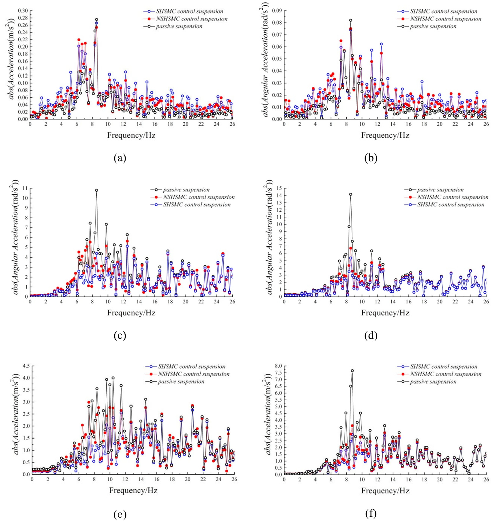
The vehicle’s dynamic state data ( ${\overset{\cdot\cdot}{z}}_{s}$ , $\overset{\cdot\cdot}{φ}$ , ${\overset{\cdot\cdot}{θ}}_{r}$ , ${\overset{\cdot\cdot}{θ}}_{l}$ , ${\overset{\cdot\cdot}{z}}_{ur}$ , ${\overset{\cdot\cdot}{z}}_{ul}$ ), which reflect the vehicle’s ride comfort and handling stability, were obtained. To further verify the effectiveness of the above-mentioned semi-active suspension control algorithm at different excitation frequencies, the fast Fourier transform (FFT) method was used to convert the vehicle dynamic state data from the time-domain to the frequency-domain while the vehicle was being driven, as shown in Figure 6.

Figure 6.

Vehicle dynamic states of semi-active suspension and passive suspension on ISO-E road: (a) Vertical acceleration of sprung mass ${\overset{\cdot\cdot}{z}}_{s}$ , (b) roll angular acceleration of sprung mass $\overset{\cdot\cdot}{φ}$ , (c) angular acceleration of right control arm ${\overset{\cdot\cdot}{θ}}_{r}$ , (d) angular acceleration of left control arm ${\overset{\cdot\cdot}{θ}}_{l}$ , (e) vertical acceleration of right un-sprung mass ${\overset{\cdot\cdot}{z}}_{ur}$ and (f) vertical acceleration of left un-sprung mass ${\overset{\cdot\cdot}{z}}_{ul}$ .

As shown in Figure 6(a) to (f),when the vehicle was being driven on an ISO-E road surface, the vibration peak values of the vehicle’s dynamic state data( ${\overset{\cdot\cdot}{z}}_{s}$ , $\overset{\cdot\cdot}{φ}$ , ${\overset{\cdot\cdot}{θ}}_{r}$ , ${\overset{\cdot\cdot}{θ}}_{l}$ , ${\overset{\cdot\cdot}{z}}_{ur}$ , ${\overset{\cdot\cdot}{z}}_{ul}$ ), which reflect the vehicle’s ride comfort and handling stability, appeared in the region of 6–10 Hz.In this peak area, compared with passive suspension, the semi-active suspension controlled by the SHSMC and NSHSMC had more effective vibration attenuation ability for the vehicle’s driving dynamic states ${\overset{\cdot\cdot}{θ}}_{r}$ , ${\overset{\cdot\cdot}{θ}}_{l}$ , ${\overset{\cdot\cdot}{z}}_{ur}$ , and ${\overset{\cdot\cdot}{z}}_{ul}$ , which can significantly enhance the vehicle’s driving safety and handling stability, without making the sprung mass vibration more severe or increasing the amplitude of the ${\overset{\cdot\cdot}{z}}_{s}$ and $\overset{\cdot\cdot}{φ}$ vibration. However, in a high-frequency region greater than 10 Hz, compared with the semi-active suspension controlled by the SHSMC and NSHSMC, the passive suspension more effectively attenuated the vibration of the driving dynamic states ${\overset{\cdot\cdot}{z}}_{s}$ and $\overset{\cdot\cdot}{φ}$ . For the vehicle’s driving dynamic states ${\overset{\cdot\cdot}{θ}}_{r}$ , ${\overset{\cdot\cdot}{θ}}_{l}$ , ${\overset{\cdot\cdot}{z}}_{ur}$ , and ${\overset{\cdot\cdot}{z}}_{ul}$ , the semi-active suspension controlled by the SHSMC and NSHSMC had the same vibration suppression ability as the passive suspension.

In the region of 6–10 Hz, compared with the NSHSMC control algorithm, the semi-active suspension controlled by the SHSMC had stronger suppression ability for the vehicle’s driving dynamic states ${\overset{\cdot\cdot}{z}}_{s}$ and $\overset{\cdot\cdot}{φ}$ . In a high-frequency region greater than 10 Hz, compared with semi-active suspension controlled by the SHSMC, the NSHSMC control algorithm had stronger suppression ability for the driving dynamic states ${\overset{\cdot\cdot}{θ}}_{r}$ , ${\overset{\cdot\cdot}{θ}}_{l}$ , ${\overset{\cdot\cdot}{z}}_{ur}$ , and ${\overset{\cdot\cdot}{z}}_{ul}$ .

Compared with the NSHSMC control algorithm, in the 6–10-Hz vibration region, the SHSMC control algorithm achieved greater improvement of the vehicle’s drive handling stability. In a high-frequency region greater than 10 Hz, the semi-active suspension controlled by the SHSMC method exerted a more adverse effect on the ride comfort.

Figure 7 shows the control force of the right side semi-active suspension controlled by the SHSMC and NSHSMC control algorithms on the ISO – -B, -D, and -F road surface.

Figure 7.

Control force of semi-active suspension.

In this study, the root mean square of the sprung-mass acceleration $rms ({\overset{\cdot\cdot}{z}}_{s})$ and the ratio a_w between the root mean square of the tire dynamic load and static tire load were adopted to further verify the ride comfort and handing stability of the suspension system, respectively, as follows:

a_{w} = \frac{rms (F_{d})}{F_{s}},

(93)

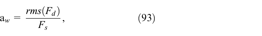
where F_d is the tire dynamic load, and F_s is the static tire load.

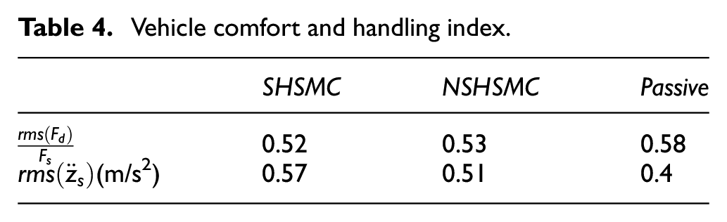
In Table 4, for an ISO-E road surface, the ride comfort and handling stability indices of a vehicle with a passive suspension and semi-active suspension system controlled by the SHSMC and NSHSMC control algorithm were obtained. Compared with passive suspension, the a_w index of the semi-active suspension system controlled by the SHSMC control algorithm decreased, while the handing stability of the semi-vehicle improved. However, the value of $rms ({\overset{\cdot\cdot}{z}}_{s})$ increased, and the vehicle ride comfort decreased. The semi-active suspension system controlled by the NSHSMC control algorithm achieved better ride comfort compared with the SHSMC control algorithm and also improved the handling stability of vehicles.

Table 4.

Vehicle comfort and handling index.

	SHSMC	NSHSMC	Passive
$\frac{rms (F_{d})}{F_{s}}$	0.52	0.53	0.58
$rms ({\overset{\cdot\cdot}{z}}_{s})$ (m/s²)	0.57	0.51	0.4

Conclusion

In this paper, a nonlinear semi-vehicle model with a McPherson semi-active suspension system was developed using Lagrange equations. The small-computational-overhead EKF and UKF state estimation algorithms were developed, and the semi-active suspension control algorithms SHSMC and NSHSMC were established. The following conclusions were drawn from this study:

(1) Based on the above-mentioned state estimation methods, the vehicle’s dynamic states were satisfactorily estimated while the vehicle was being driven on a rough road surface. Compared with the small-computational-overhead EKF algorithm, the estimation of these variables based on the UKF algorithm was more accurate. However, the UKF algorithm requires longer computation time for each step compared with the EKF algorithm.

(2) Compared with the NSHSMC control algorithm, in the 6–10-Hz vibration region, the SHSMC control algorithm achieved greater improvement of the vehicle’s drive handling stability. In a high-frequency region greater than 10 Hz, the semi-active suspension controlled by the SHSMC control algorithm exerted a more adverse effect on the ride comfort.

Footnotes

Appendix

C = {[\begin{array}{l} 0, 1, 0, 0, 0, 0, 0, 0 \\ \frac{\partial f_{1}}{\partial x_{1}}, \frac{\partial f_{1}}{\partial x_{2}}, \frac{\partial f_{1}}{\partial x_{3}}, \frac{\partial f_{1}}{\partial x_{4}}, \frac{\partial f_{1}}{\partial x_{5}}, \frac{\partial f_{1}}{\partial x_{6}}, \frac{\partial f_{1}}{\partial x_{7}}, \frac{\partial f_{1}}{\partial x_{8}} \\ 0, 0, 0, 1, 0, 0, 0, 0 \\ \frac{\partial f_{2}}{\partial x_{1}}, \frac{\partial f_{2}}{\partial x_{2}}, \frac{\partial f_{2}}{\partial x_{3}}, \frac{\partial f_{2}}{\partial x_{4}}, \frac{\partial f_{2}}{\partial x_{5}}, \frac{\partial f_{2}}{\partial x_{6}}, \frac{\partial f_{2}}{\partial x_{7}}, \frac{\partial f_{2}}{\partial x_{8}} \\ 0, 0, 0, 0, 0, 1, 0, 0 \\ \frac{\partial f_{3}}{\partial x_{1}}, \frac{\partial f_{3}}{\partial x_{2}}, \frac{\partial f_{3}}{\partial x_{3}}, \frac{\partial f_{3}}{\partial x_{4}}, \frac{\partial f_{3}}{\partial x_{5}}, \frac{\partial f_{3}}{\partial x_{6}}, \frac{\partial f_{3}}{\partial x_{7}}, \frac{\partial f_{3}}{\partial x_{8}} \\ 0, 0, 0, 0, 0, 0, 0, 1 \\ \frac{\partial f_{4}}{\partial x_{1}}, \frac{\partial f_{4}}{\partial x_{2}}, \frac{\partial f_{4}}{\partial x_{3}}, \frac{\partial f_{4}}{\partial x_{4}}, \frac{\partial f_{4}}{\partial x_{5}}, \frac{\partial f_{4}}{\partial x_{6}}, \frac{\partial f_{4}}{\partial x_{7}}, \frac{\partial f_{4}}{\partial x_{8}} \end{array}]}_{({\vec{x}}_{e}, z_{l} = 0, z_{r} = 0, u_{r} = 0, u_{l} = 0)}

{[\begin{matrix} D_{1} \\ D_{2} \\ E_{1} \\ E_{2} \end{matrix}]}^{T} = {[\begin{matrix} \begin{matrix} 0 \\ \frac{\partial f_{1}}{\partial z_{l}} \\ 0 \\ \frac{\partial f_{2}}{\partial z_{l}} \\ 0 \\ \frac{\partial f_{3}}{\partial z_{l}} \\ 0 \\ \frac{\partial f_{4}}{\partial z_{l}} \end{matrix} & \begin{matrix} 0 \\ \frac{\partial f_{1}}{\partial z_{r}} \\ 0 \\ \frac{\partial f_{2}}{\partial z_{r}} \\ 0 \\ \frac{\partial f_{3}}{\partial z_{r}} \\ 0 \\ \frac{\partial f_{4}}{\partial z_{r}} \end{matrix} & \begin{matrix} 0 \\ \frac{\partial f_{1}}{\partial u_{l}} \\ 0 \\ \frac{\partial f_{2}}{\partial u_{l}} \\ 0 \\ \frac{\partial f_{3}}{\partial u_{l}} \\ 0 \\ \frac{\partial f_{4}}{\partial u_{l}} \end{matrix} & \begin{matrix} 0 \\ \frac{\partial f_{1}}{\partial u_{r}} \\ 0 \\ \frac{\partial f_{2}}{\partial u_{r}} \\ 0 \\ \frac{\partial f_{3}}{\partial u_{r}} \\ 0 \\ \frac{\partial f_{4}}{\partial u_{r}} \end{matrix} \end{matrix}]}_{({\vec{x}}_{e}, z_{l} = 0, z_{r} = 0, u_{l} = 0, u_{r} = 0)}

H = [\begin{matrix} 0 & 1 & 0 & 0 & 0 & 0 & 0 & 0 \\ 0 & 0 & 0 & 0 & 1 & 0 & 0 & 0 \\ 0 & 0 & 0 & 0 & 0 & 0 & 1 & 0 \end{matrix}]

Acknowledgements

We thank LiwenBianji, Edanz Editing China (), for editing the English text of a draft of this manuscript.

Handling Editor: James Baldwin

Declaration of conflicting interests

The author(s) declared no potential conflicts of interest with respect to the research, authorship, and/or publication of this article.

Funding

The author(s) received no financial support for the research, authorship, and/or publication of this article.

ORCID iDs

Wang Xin

Gu Liang

References

Stensson

Asplund

Karlsson

The nonlinear behaviour of a MacPherson Strut wheel suspension. J Veh Syst Dyn 1994; 23: 85–106.

Hong

Jeon

Yoo

, et al. A new model and an optimal pole-placement control of the MacPherson suspension system. SAE paper 1999-01-1331:1, 1999.

Shojaeefard

Khalkhali

Yarmohammadisatri

An efficient sensitivity analysis method for modified geometry of Macpherson suspension based on Pearson correlation coefficient. J Veh Syst Dyn 2017; 55: 827–852.

Fallah

Bhat

Xie

WF.

New model and simulation of Macpherson suspension system for ride control applications. J Veh Syst Dyn 2009; 47: 195–220.

Fallah

Bhat

Xie

. New nonlinear model of Macpherson suspension system for ride control applications. In: American control conference, Seattle, WA, 11–13 June 2008. New York: IEEE.

Karnopp

Croby

Harwood

RA.

Vibration control using semi-active force generators. J Eng Ind 1974; 96: 619–626.

Rao

LVVG

Narayanan

. Sky-hook control of nonlinear quarter car model traversing rough road matching performance of LQR control. J Sound Vib 2009; 323: 515–529.

Nie

Yang

Jiang

Passive skyhook suspension reduction for improvement of ride comfort in an off-road vehicle. IEEE Access 2019; 7: 150710–150719.

Liu

Chen

Yang

, et al. General theory of skyhook control and its application to semi-active suspension control strategy design. IEEE Access 2019; 7: 101552–101560.

10.

Liu

Ren

Chen

, et al. Feedback linearization Kalman observer based sliding mode control for semi-active suspension systems. IEEE Access 2020; 8: 1–20.

11.

Singh

Arat

Taheri

Literature review and fundamental approaches for vehicle and tire state estimation. J Veh Syst Dyn 2019; 11: 1643–1665.

12.

Qin

Langari

A new modeling algorithm based on ANFIS and GMDH. J Intell Fuzzy Syst 2015; 29: 1321–1329.

13.

Qin

YC.

Research on vehicle semi-active suspension system based on road profile estimation. PhD Thesis, Beijing Institute of Technology, China, 2016.

14.

Doumiati

Victorino

Lechner

Observers for vehicle tire/road forces estimation: experimental validation. J Veh Syst Dyn 2010; 48: 1345–1378.

15.

Hongbin

Sizhong

Zhicheng

. Model of excitation of random road profile in time domain for a vehicle with four wheels. In: International conference on mechatronic science, Jilin, China, 19–22 August 2011. New York: IEEE.

16.

Bogsjö

Coherence of road roughness in left and right wheel-path. J Veh Syst Dyn 2008; 46: 599–609.

17.

Bogsjö

Evaluation of stochastic models of parallel road tracks. J Probab Eng Mech 2007; 22: 362–370.

18.

Janesick

JR.

Scientific charge-coupled devices. Washington, DC: The International Society for Optical Engineering, 2000.

19.

Julier

Uhlmann

. A new extension of the Kalman filter to nonlinear systems. In: Proceedings of the Aerosense: The 8th international symposium on aerospace/defense Sensing, simulation and controls, Orlando, Florida, April 1997. Bellingham, WA: SPIE, Multi Sensor Fusion, Tracking and Resource Management II, Society of Photo-Optical Instrumentation Engineers.

20.

Wan

Merwe

RVD

. The unscented Kalman filter for nonlinear estimation. In: Proceedings of the IEEE 2000 adaptive systems for signal processing, communications, and control symposium (Cat. No.00EX373), Lake Louise, AB, Canada, 4 October 2000. New York: IEEE.

Comparative simulation study on two estimation methods and two control strategies for semi-active suspension

Abstract

Keywords

Introduction

Problem statement

State of the art

Contribution

Mathematical modeling

Road excitation

Road roughness function built using harmonic superposition method

Coherence of bilateral track excitation

New nonlinear semi-vehicle suspension model

Equations of motion

Vehicle dynamic state estimator

Small-computational-overhead EKF method

Unscented Kalman estimation method

Estimation of road process noise variance matrices Q and measurement noise variance matrices R

State estimation results

Nonlinear reference mode sliding mode control algorithm

Skyhook sliding mode control algorithm (SHSMC)

New nonlinear Skyhook-SMC control algorithm

Simulation results for semi-active suspension controller

Conclusion

Footnotes

Appendix

Acknowledgements

Declaration of conflicting interests

Funding

ORCID iDs

References